1. Introduction
AC motor drives are currently widely used in both industrial systems and mobility-related tasks. In connection with the key task performed by the drives, it is important to ensure machine reliability and early warning of possible failure of drive system components. This task is related to highly developed technical diagnostics covering power supply and drive control systems, as well as the motors themselves and elements of the kinetic chain. Currently, designed diagnostic systems ensure control of the technical condition of the object based on information obtained from additional measurement systems. Therefore, a key point in the detection and prediction of defects is to obtain data that contain information about the technical condition of the object [
1].
The information processing cycle in a classic diagnostic system includes measuring physical signals and transferring data to a superior system, in which the features are determined and then the technical condition of the tested object is assessed. It should be clearly stated that, for effective fault diagnosis, it is crucial to ensure high-quality data acquisition and transfer them to the superior system without losing information. Any interference between the measurement and the computational systems may result in an incorrect assessment of the condition of the object, which may have critical consequences for the subsequent operation of the drive. Therefore, in priority systems, special methods are used to check the accuracy of the diagnostic information transmitted. These techniques most often significantly limit the parameters of the data acquisition system (sampling frequency and data packet size) [
2,
3]. Therefore, superior computational systems must be adapted to a limited amount of information. This fact influences the need to adapt the techniques for assessing the technical condition of the object under consideration.
The currently used diagnostic systems focus mainly on multistage processing of measurement data and full automation of the damage detection process [
3]. This automation is achieved by fully [
4,
5] or partially [
6,
7] supporting the system with artificial intelligence techniques. For many years, the dominant diagnostic method was the combination of classical symptom extraction using methods to analyze signals measured in the time domain [
8,
9,
10,
11], as well as frequency [
12,
13,
14,
15] or time–frequency analysis [
16,
17,
18,
19] with simple neural structures. This approach was characterized by low computational overhead, which made it easy to practice implementation on microprocessors. The developed sets of damage symptoms were sent in the form of vectors to the input of the network, which allowed their multidimensional approximation (multilayer perceptron) [
20,
21], data classification (self-organizing Kohonen maps) [
22,
23], or data assignment to known patterns (recurrent Hopfield networks) [
24]. However, these solutions are limited by the data acquisition system used, necessitating a long measurement time [
16]. Moreover, it should be clearly emphasized that the symptom extraction methods did not provide adequate precision and completely excluded the possibility of detection in transient states [
25,
26].
The solution to these limitations is the direct analysis of signals measured by deep neural structures [
27,
28]. Deep networks are successfully used in the diagnosis of electrical machine failures, characterized by high precision and a fast response to defects [
29]. This fact results from the possibility of automatic extraction of input information features and assignment to one of the known classes. For this purpose, they require the use of an extensive network architecture and large sets of training data, which is why they are computationally difficult, which is a disadvantage of deep networks compared to classical structures. In addition, the selection of deep network parameters requires control of the generalizability of the network that contains a significant number of neural connections. These difficulties are minimized by the use of stochastic weight adaptation techniques, as well as the development of neural structures based on the transfer of features to a pretrained network [
2,
30,
31] (transfer learning).
The diagnostic approach proposed in this article combines the classical structure of an SOM with a CNN derived from deep learning. The system operation uses analytical methods to extract fault symptoms based on MCSA and SCA. The limitation of the number of signal samples measured on the object, assumed in the research, is particularly important. The applied technique ensures precise and fast detection and localization of stator winding turn short circuits in the induction motor based solely on 600 samples of phase current signals. Moreover, the combination of the SOM classification capabilities based on a small dataset and automatic feature extraction by the convolutional neural network ensured correct assessment of the technical condition in both steady and transient states.
Reliable operation under dynamically changing load torque conditions was a key requirement for the system. The main difference between the proposed algorithm and conventional deep learning methods lies in the use of a single convolutional layer, which significantly reduces the number of parameters. In the proposed framework, the convolutional network serves as a digital filter that defines the feature space over the matrices of Euclidean distance measures. Furthermore, its application enabled effective classification of the fault type. The deep-learning-based diagnostic approaches described in the literature typically focus on transferring the entire information processing chain into a deep network. However, due to the limitations of the computational system, it was not feasible to apply complex deep structures capable of directly extracting features and performing classification. Additionally, these deep learning applications often require large training datasets, long training times, and the availability of adequate computational resources—all of which pose constraints for practical implementation. The developed algorithm is based on an initial classification of fault symptoms obtained through analytical methods using an SOM. Consequently, a CNN was used for analyzing matrices containing Euclidean distance measures.
2. Measurements
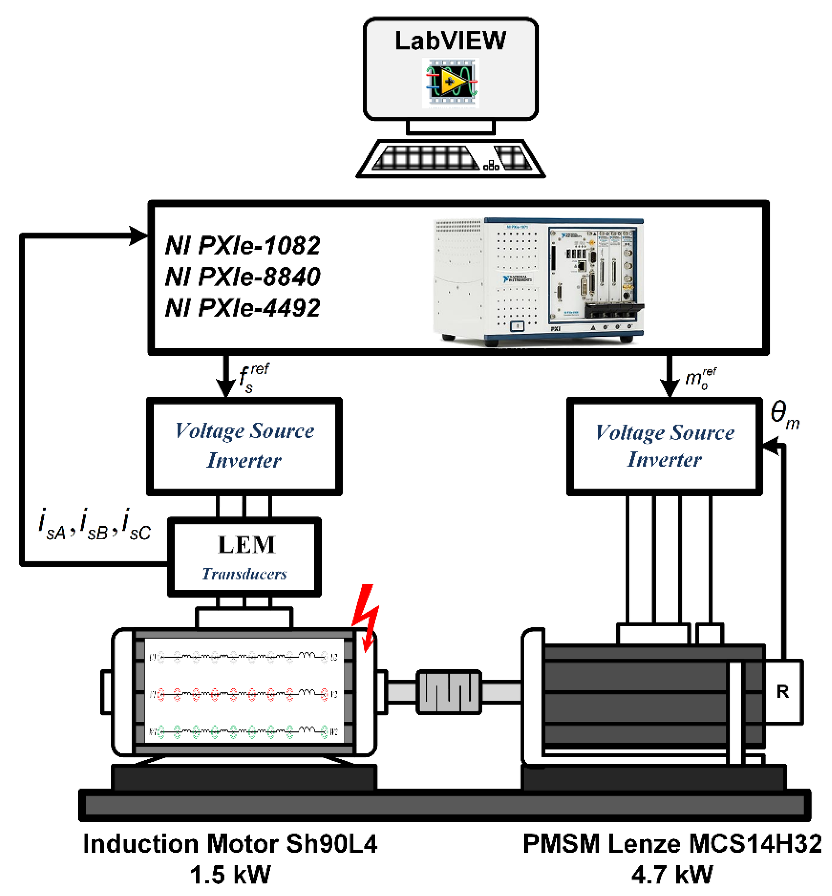
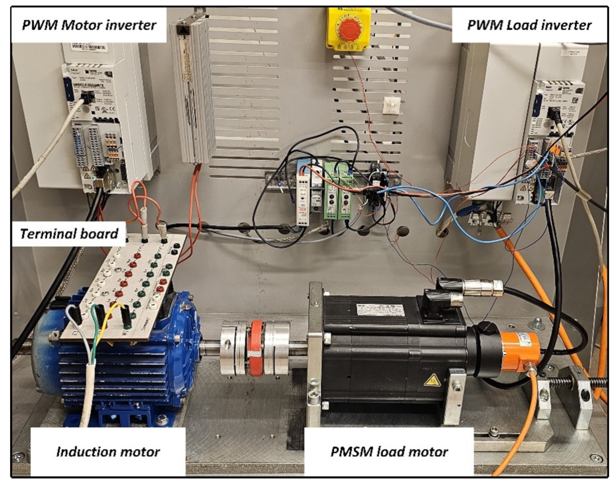
The experimental studies were carried out on a test bench shown in
Figure 1. This stand consists of two motors: a tested 1.5 kW induction motor and a 4.7 kW permanent magnet synchronous motor (PMSM) serving as a load generator. Both motors are controlled by Lenze frequency converters, with the physical arrangement shown in
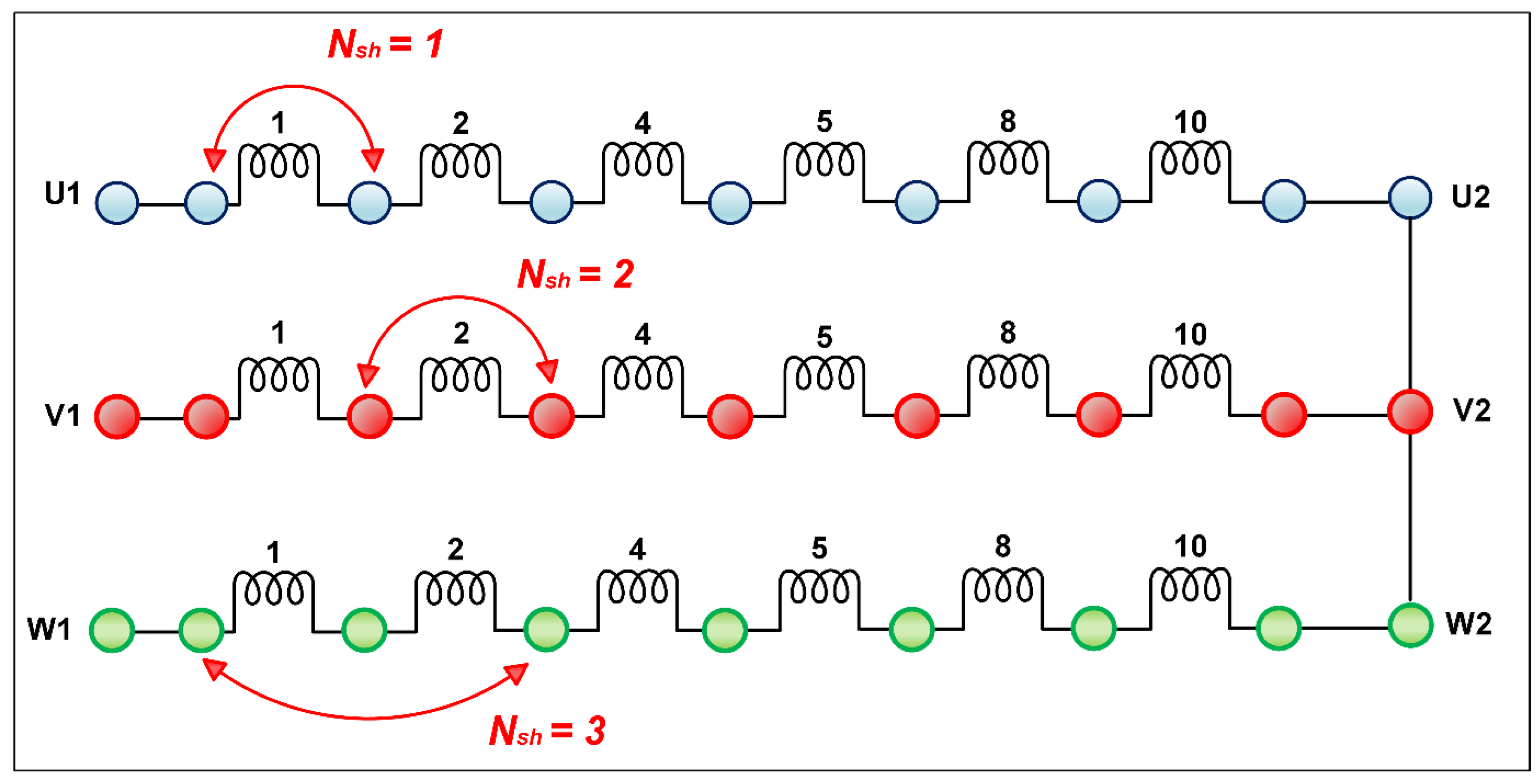
Figure 2. The induction motor features a specially rewound stator that enables physical simulation of inter-turn short circuits in each phase. The modified winding allows short-circuiting from one to several dozen turns through a dedicated terminal board, where faults are implemented by connecting the appropriate terminals (
Figure 3). The 1.5 kW induction motor (Indukta Sh90L-4) utilized for validation features a 36-slot stator with three-phase windings. Each phase comprises 312 total turns, distributed across 6 series-connected coils, with each coil having 52 turns. For precise fault simulation, 1 selected coil per phase was modified to allow individual turn terminals to be brought out to a connection board. This enabled the accurate short-circuiting of 1 to 5 turns, representing 0.32% to 1.6% of the total phase turns. This setup allowed for the emulation of both incipient (1–2 turns) and developing (3–5 turns) inter-turn short-circuit faults. The IM rated parameters are provided in
Table A1.
The stator phase currents are measured with multirange current tranducers (LEM LA 25-NP) and are transferred to the data acquisition system, which is the data acquisition card (DAQ NI-PXI-4492, National Instruments). This measurement card is placed inside the industrial PC—NI PXI 1082. The diagnostic application is developed in LabVIEW programming environment.
The tested induction motor operated under scalar control (U/f = const) at 50 Hz supply frequency with 10 kHz PWM modulation. Diagnostic systems designed for use in safety-critical drives have several requirements in terms of time and detection performance. At the same time, some limitations are imposed on these systems as a result of the available measurement systems or the computational capacity of the processor. As this study concerns such a system, the required measurement parameters are the following: a sampling rate of 10 kHz and a maximum of 750 samples. The load was step-changed every 6 s from 0.3 to 1.0 (—nominal value of load torque) for each fault level, from 0 to 5 shorted turns in one winding coil. The number of shorted turns was limited to maximum 5, which accounted for 1.6% of all turns in one phase. This is due to the realization of tests without an additional short-circuit current-limiting resistor. Then, from the data obtained, parts corresponding to the steady states were segmented, which were used to extract symptoms and prepare the input data vector for the network. Furthermore, measurements were carried out, during which 1 to 3 turns in the selected phase were temporarily short-circuited to verify the performance of the system under transient conditions.
3. Signal Processing
The purpose of the designed diagnostic system is to perform damage detection by recognizing the phase in which the damage occurred and classifying its degree. As shown in
Figure 4, the input data are processed by various algorithms to obtain a damage classification based on the measured phase current data.
Diagnostic systems designed for use in safety-critical drives have several requirements in terms of time and detection performance. At the same time, some limitations are imposed on these systems as a result of the available measurement systems or the computational capacity of the processor. As this study concerns such a system, the required measurement parameters are the following: a sampling rate of 10 kHz and a maximum of 750 samples.
Measurements were carried out on an induction motor supplied by an inverter ( = 50 Hz). The load was step-changed every 6 s from 0.3 to 1.0 (—nominal value of load torque) for each fault level, from 0 to 5 shorted turns in one winding coil. Then, from the data obtained, parts corresponding to the steady states were segmented, which were used to extract symptoms and prepare the input data vector for the network. Furthermore, measurements were carried out, during which 1 to 3 turns in the selected phase were temporarily short-circuited to verify the system performance under transient conditions.
Due to the limitations of the measurement system, specifically concerning sampling frequency and the available data buffer size, it was decided to use 3 periods (600 samples) of the measured signal to extract the maximum amount of information. It was also due to the need for a smooth transition between the start and end of the recorded signal used in the following algorithm. The 600 samples obtained in this way would lead to an unreadable FFT due to the low resolution and the possibility that imperfections in the actual signal would have a large impact on the results. To address these problems, it was decided to increase the sampling of the signal by multiplying it to obtain 6 s of the signal. The original 3 periods were copied and anchored to the end of the signal so that a signal of 60,000 samples was obtained (Algorithm 1). Varying the measurement sample time significantly impacts diagnostic accuracy. While increasing the acquisition time (e.g., to 6 or 9 periods) can enhance spectral resolution and symptom clarity, thereby improving network precision, it would counteract the objective of the system for rapid fault detection, especially in transient states where a longer signal might not be stationary. Conversely, reducing the acquisition time below 0.06 s would lead to insufficient spectral resolution for accurate symptom extraction, potentially causing erroneous classifications. Therefore, the 0.06 s (3-period) duration was selected as a balanced approach, providing sufficient information for robust diagnostics while maintaining a critically short acquisition window. To verify the symptoms obtained as a result, an analysis was also carried out for a 6 s signal measured in steady state.
| Algorithm 1 Extracting and Extending a 3-Period Sinusoidal Signal |
Require , , : the measured sample of the stator phase currents Ensure: , , : phase current signal composed of 3 multiplied periods 2:
Extract 3 periods starting from : 3: Extend the signal for phase A (for the other phases calculated analogously):
|
4. Symptom Extraction
The occurrence of a stator winding fault causes a significant magnetic imbalance, which appears in the current signal. This signal becomes asymmetrical and reveals characteristic harmonics, possible symptoms to detect this fault. In this study, two methods of symptom extraction were used: motor current signature analysis (MCSA) and symmetrical component analysis (SCA).
MCSA [
16,
32,
33] is a prevalent method for the online detection of motor faults. This technique aims to identify specific fault-related components in the stator-current spectrum. However, in the case of converter drives, additional complications arise in the form of distorted current signals and variable operating conditions (regulated frequency and amplitude of the supply voltage), which may make symptom extraction more difficult.
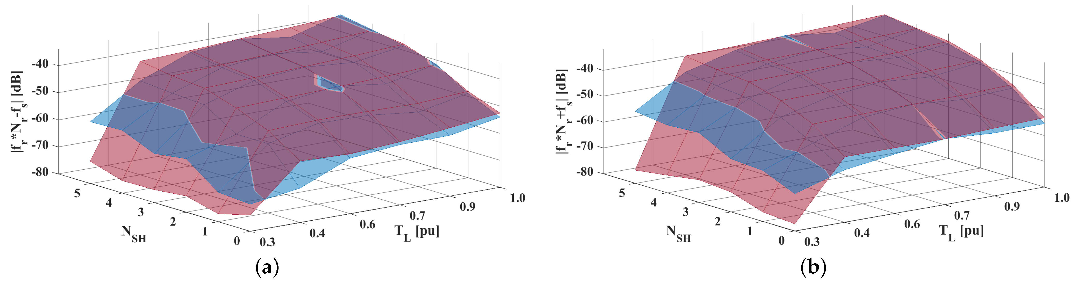
During the analysis, the largest changes in amplitude due to the occurrence of a fault appeared at frequency
, which can be written with the formula
where
is the rotational frequency,
is the number of rotor slots, and
is the supply frequency.
This frequency is related to the appearance of static eccentricity [
32]. This type of fault occurs when the rotor is not coaxial with the housing, resulting in an imbalance in the air gap between the rotor and the stator. The unbalanced air gap leads to an asymmetry in the magnetic-field distribution, resulting in harmonics in the supply current. Winding short circuits also cause local disturbances in the magnetic field, which can affect the distribution of magnetic forces in a way similar to static eccentricity. As a result, both static eccentricity and short-circuiting can lead to an increase in the amplitude of frequency harmonics.
Under steady-state conditions, the imbalance in three-phase systems can be assessed using the widely recognized method of SCA [
34]. This approach involves transforming the three-phase stator currents of induction motors into a symmetrical component coordinate system through Fortescue’s complex transformation:
where
,
, and
denote the steady-state stator phase currents for phases A, B, and C;
,
, and
represent the zero-sequence, positive-sequence, and negative-sequence components of the steady-state stator current; and a is defined as
.
In three-phase induction motors, the zero-sequence component of the current does not exist, so the calculation of the symmetrical components is reduced to the calculation of
and
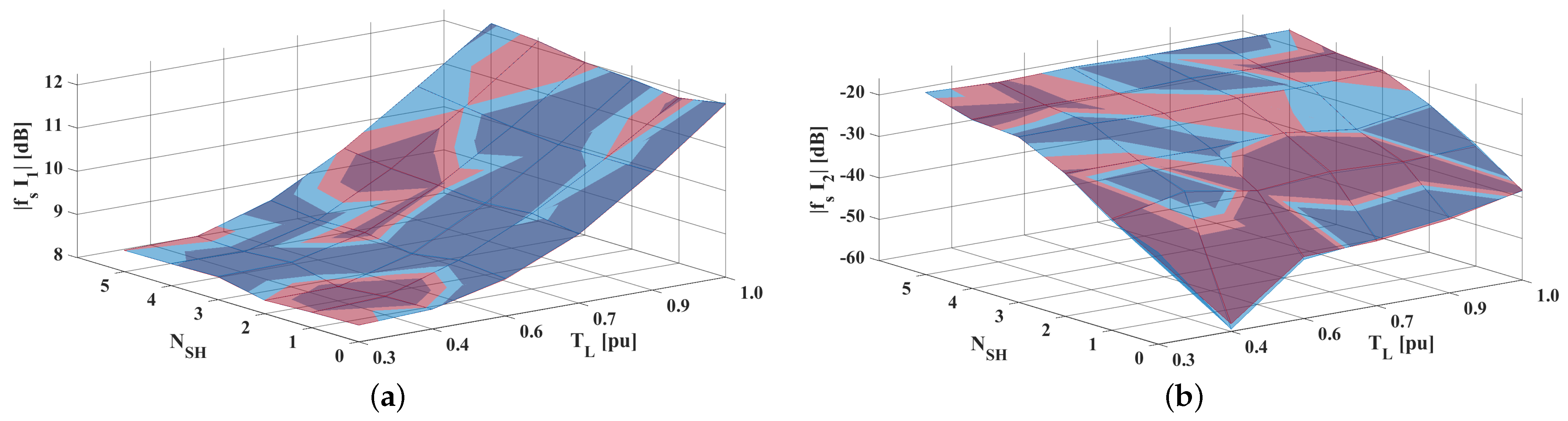
. By comparing the information carried by the selected symptoms for both signals (
Figure 5 and
Figure 6), it can be seen that, despite the significantly smaller number of samples, the fault information is retained for the signal merged from three periods. This allows us to provide an input signal for the designed network while reducing the number of samples of the measured signal needed. Based on the analysis of the measurement data with MCSA and SCA, diagnostic symptoms were extracted and formed as an input vector for the SOM network (Algorithm 2).
| Algorithm 2 Symptom Extraction Using MCSA and SCA for SOM Network Input |
Require , , : phase current signal composed of 3 multiplied periods; : number of rotor slots; : supply frequency Ensure: Symptom vector S for SOM network 1: MCSA Analysis: Computation of MCSA-related symptoms based on Equation ( 1): 2: SCA Analysis: Computation of SCA-related symptoms for the positive sequence component and the negative sequence component (Equation ( 2)): 3: Form the Symptom Vector:
|
The diagnostic system primarily utilizes changes in the characteristic amplitudes for the stator fault and the negative sequence component of the stator current . While other magnetic imbalances, such as rotor faults or unbalanced supply voltages, can also affect the current signal, they are differentiated as follows: rotor faults generate slip-dependent components () in the stator current spectrum, which do not significantly affect the symmetrical component or overlap with the stator winding fault signatures (). In the context of VFD-fed systems used in this study, supply voltage unbalance is practically mitigated by the inherent voltage balancing capability of the inverter. This combined monitoring of fault-specific frequencies and symmetrical components provides robustness against false alarms from these other common sources of imbalance.
5. Neural-Network-Based Classifier
The use of an SOM is due to its good classification ability based on relatively small sets of training data, which was demonstrated, among others, in [
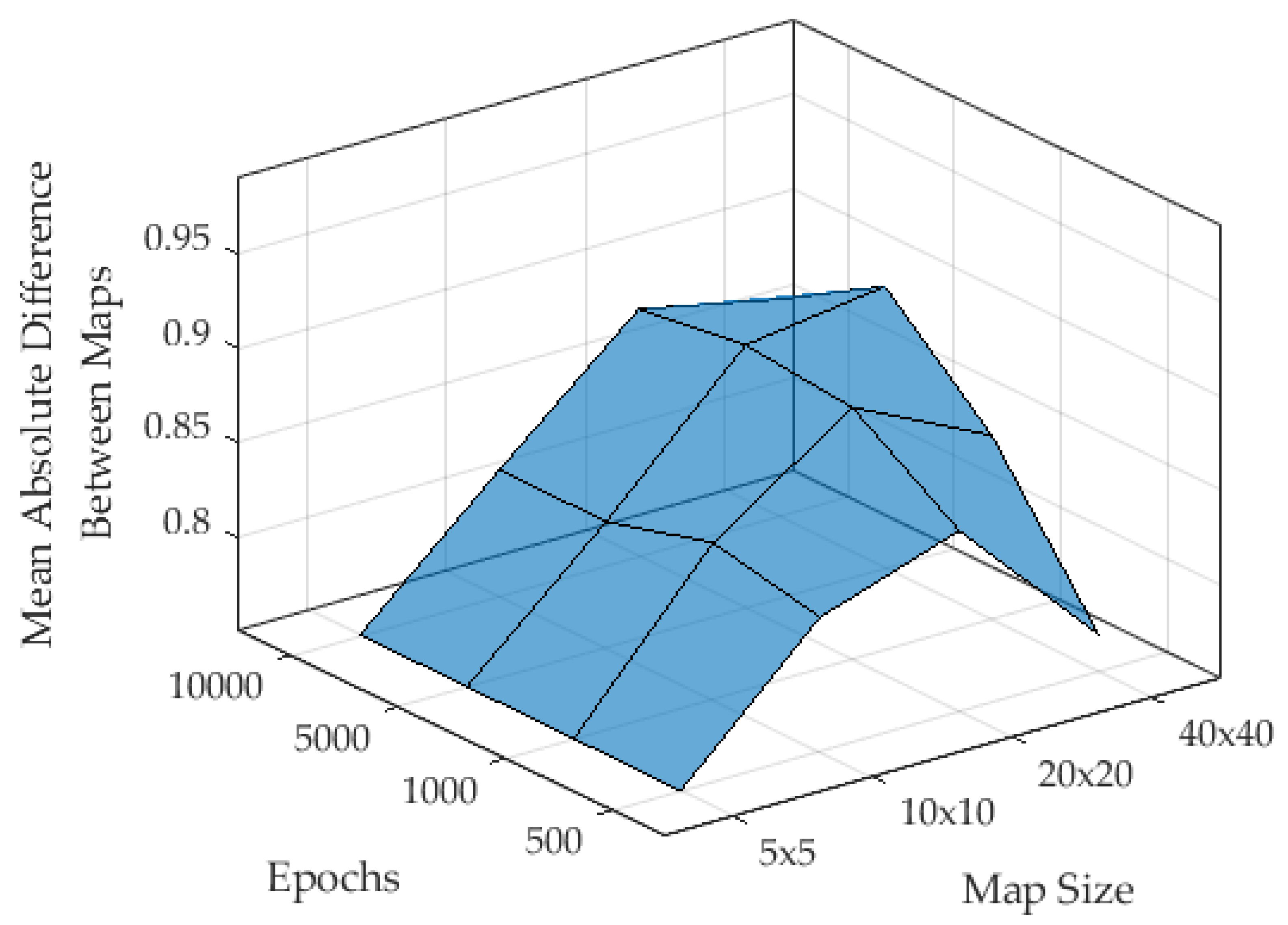
35]. SOM-based system analysis consists mainly of assessing the activity of neurons distributed on the neuron grid. The active neurons for a given input vector are selected based on the minimum distance between the elements of the input vector and all neurons in the network. However, in this research, instead of solely focusing on the active neurons, the information about the input features is extensively preserved and utilized through the complete set of Euclidean distance measures. This full matrix of distances, representing the relationships between the input vector and all neurons on the map, is then leveraged for diagnostic purposes. This comprehensive approach to utilizing the Euclidean distance measures means that standard SOM quality metrics, which are typically based on the concept of winning neurons and map topology, are not directly applicable. However, precisely because we have access to the information contained within every neuron on the map through these Euclidean distance measures, we can utilize other advanced tools for classification, such as a CNN, as demonstrated in our example. This allows for a deeper analysis of the spatial relationships and patterns within the data that might not be fully captured by only the winning neuron. In the research, this process of training the SOM to generate these Euclidean distance matrices constituted the first stage of neural computation. In analyzing the spatial structure of the self-organizing Kohonen network, various map sizes, ranging from 5 × 5 to 40 × 40 with a rectangular topology, were investigated (
Figure 7).
Figure 7 displays the outcome of an analysis aimed at selecting optimal SOM parameters (map size and training epochs for the initial SOM training detailed in Algorithm 3) by evaluating the dissimilarity in the response of the SOM to a healthy motor state (
= 0) versus a state with five shorted turns (
= 5). For each evaluated combination of map size and training epochs, a single SOM was trained. Subsequently, using this specific trained SOM, two Euclidean distance maps were generated: one by inputting the symptom vector for the
= 0 case and another by inputting the symptom vector for the
= 5 case. Each cell in these distance maps represents the Euclidean distance between the respective input symptom vector and the weight vectors of all neurons in the trained SOM. The Z-axis in
Figure 7, labeled ‘Mean Absolute Difference Between Maps’, is the average of the cell-by-cell absolute differences calculated between these two generated Euclidean distance maps (the one for
= 0 and the one for
= 5, both derived from the same trained SOM). A higher value on this Z-axis signifies that the trained SOM produces more distinct output patterns for these two extreme conditions, a characteristic that is desirable for achieving robust fault classification. The selection of this range was based on previous research and experience in applying SOM networks to induction motor fault diagnostics. The 20 × 20 map size was ultimately chosen as it offered the most advantageous balance of performance and stability among the tested configurations. Specifically, it yielded a substantially larger mean absolute difference between the maps for healthy (
= 0) and faulty (
= 5) conditions compared to the smaller 5 × 5 and 10 × 10 maps, indicating better potential for distinguishing between states. While the 5 × 5 map also showed high stability across training epochs, its lower mean difference values made it less optimal for classification. Furthermore, when compared to the larger 40 × 40 map, the 20 × 20 map demonstrated more desirable stability; the 40 × 40 performance of the map peaked and then declined with increased epochs, suggesting a tendency towards overfitting, whereas the 20 × 20 performance of the map remained relatively consistent and high once an adequate number of epochs was reached.
| Algorithm 3 The Process of Training the SOM Network |
Require: symptom vector 1: Initialization: Map_size = (Map_size) ▹ Initialization of weight coefficients 2: for epochs = 1 to 1000 do 3: For phase A, calculate the Euclidean distance : 4: Identification of the winner neuron c: 5: Adaptation of the weights using the WTM method:
where
is the neighborhood function; is the learning rate; is the distance between the winning neuron c and the m-th neuron.
6: Adaptation of and the neighborhood radius R. 7: end for
|
Compared to deeper CNNs that might operate directly on feature vectors, SOM offers lower computational complexity and provides a structured input for the subsequent CNN. Additionally, SOM transforms the raw feature vector into a spatially organized representation (Euclidean distance map) that enhances the performance of the subsequent CNN classifier by presenting the information in a more discernible pattern for automatic feature extraction. The process of training the designed network was carried out only for phase A (Algorithm 3), and then the Euclidean distances for all three phases were calculated and a 3D image was created from them (Algorithm 4), which was the input of the CNN.
| Algorithm 4 Euclidean Distances to 3D Image Conversion |
Require , , : matrix of Euclidean distances for phases A, B, C 1: for to number of training samples do 2: end for
|
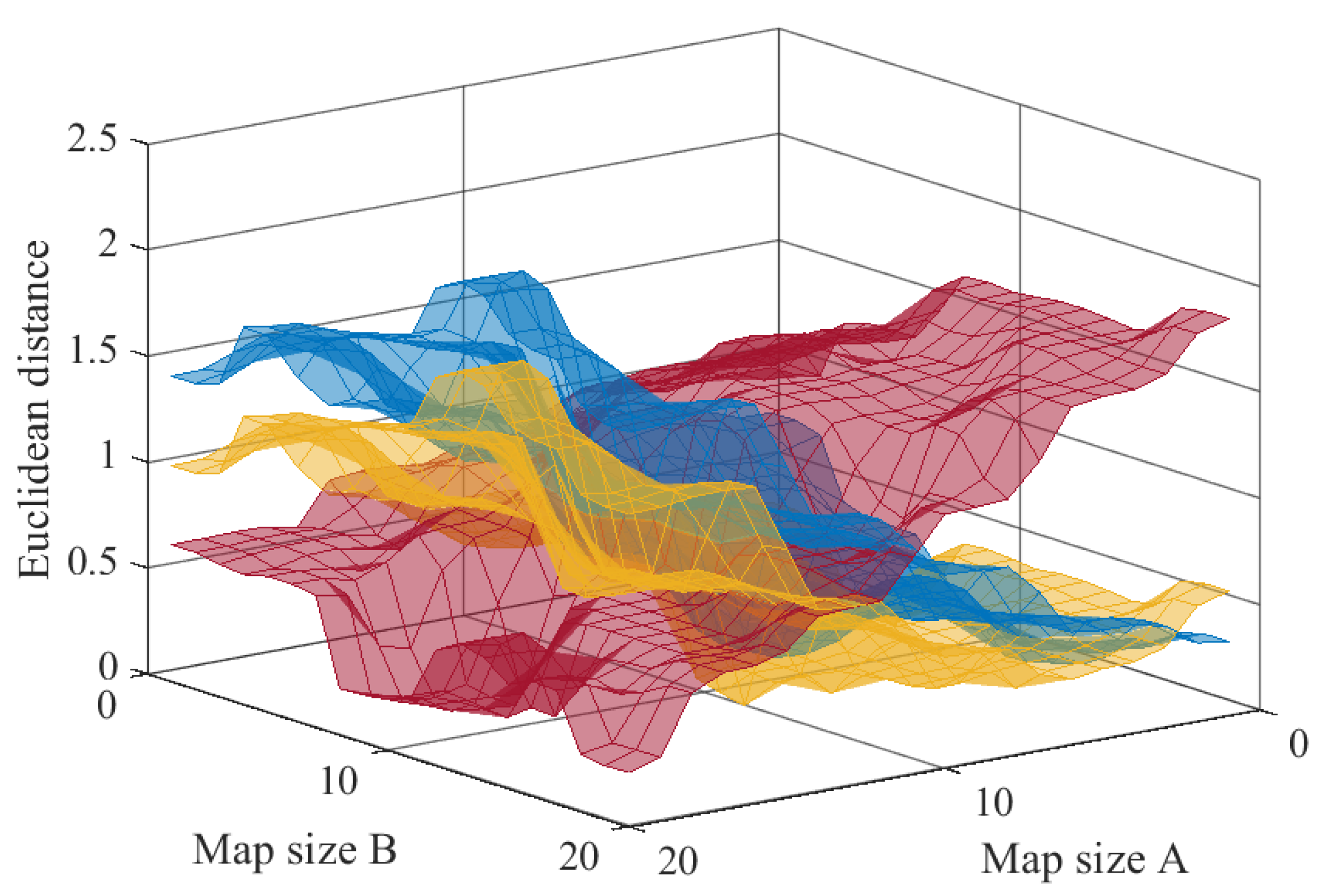
Based on the Euclidean distance measures determined between the input vectors and the SOM neurons for different degrees of defect (Algorithm 3), sets of matrices were generated for each stator phase. It should be emphasized that the SOM was trained only for phase A. However, during operation, the system simultaneously monitors all three phase currents (, , and ), and separate distance maps are generated for each phase. This is possible because faults induce similarly structured changes in the affected phase current, regardless of which phase is involved. Therefore, an SOM trained on one phase generalizes well to the others and can be used as a common reference in generating Euclidean distance maps for all three phases. The final classification, determining both the presence and specific location of the fault, is then derived by analyzing the combined outputs from all three phases.
As can be seen in
Figure 8, the increase in the degree of stator defect affects the activation of the neurons distributed on the map. Due to this, it is possible to determine the degree of defect by analyzing the distribution of distance measures in the plane. This process is very difficult due to different machine operating conditions (changes in rotational speed or load). This results from a similar impact of changes in operating conditions and stator damage on the values of phase currents. Moreover, taking into account the need to operate the system in transient conditions, the use of only the analysis of the Euclidean measure map for individual stator phases does not provide high precision in detecting defects at an early stage. Therefore, to automate the process and determine informal relationships between map areas, it was decided to use a CNN simplified only to a single convolutional and classification layer. This approach was based on the high efficiency of the CNN in extracting features recorded in data with a regular structure, such as multidimensional matrices. Therefore, in the next step, conversions of 3 Euclidean distance measurement matrices to a single three-dimensional matrix were performed according to Algorithm 4.
Based on the input data developed, the CNN training process (Algorithm 5) was carried out based on a data package containing 96 samples. While the dataset size of 96 samples might appear limited, the ratio of training samples to trainable parameters (0.032) compares favorably to recent studies in the field (0.0024 in [
36], 0.0218 in [
37], and 0.0117 in [
38]), indicating a robust balance for the complexity of the network. The applied CNN structure used only a single set of convolutional layers. Such a large simplification resulted in high dynamics of the training process and was possible thanks to the use of signal preprocessing (extraction of symptoms using MCSA and SCA analyses). The training process was carried out following the stochastic gradient descent algorithm. During the adaptation of weight coefficients, the loss function is analyzed to stop the process at the moment of achieving process convergence. In addition, rejection layers were used to ensure the maintenance of the generalization ability of the network, which is of particular importance for a diagnostic system verified on a real object. The output layer was a perceptron with the number of neurons corresponding to the number of recognized damage classes (16 classes: 1—unfaulty state; 2—16 inter-turn short circuits of 1–5 shorted turns in phases A, B, and C). The parameters of the SOM and CNN neural structures, as well as the training process, are listed in
Appendix A.
| Algorithm 5 CNN Training Process |
Require : set of images, y: set of labels 1: Initialization: Initialize network structure layers (convolution, normalization, pooling, activation function, dropout, fully connected, softmax, and classification). Initialize training parameters (training algorithm, number of epochs, initial learning rate, mini-batch size, momentum coefficient, learning rate schedule, learning rate drop period, learning rate drop factor, and L2 regularization).
2: for epoch = 1 to 200 do 3: Step 1: 4: Step 2: 5: for each mini-batch in B do 6: Step 2.1: The execution of forward pass through the network and save its response . 7: Step 2.2: Calculation of cross-entropy loss using and y. 8: Step 2.3: Execution of backpropagation and memorizing the calculated gradients . 9: Step 2.4: Adaptation of the network weights of the network. 10: end for 11: Step 3: 12: if epoch is a multiple of the learning rate drop period then Adaptation of the learning rate. 13: end if 14: end for
|
The final classification of the degree of damage and the phase in which the damage occurred was analyzed using prepared fault symptoms. Based on the collected data, training, validation, and test sets were determined for a system based on 3 measurement periods (Net-3period) and training and test sets for a reference system based on 6 measurement seconds (Net-6s). For the system using 3 measurement periods, three different non-overlapping locations were selected from each steady-state signal, and each location went into one of the three sets. For the system based on 6 s of measurement, it was decided to allocate the measurements collected for loads of 0.3, 0.6, and 1.0 to training, leaving the measurements collected for loads of 0.4, 0.7, and 0.9 to testing the system. In addition to the standard classification of the data, it was also decided to realize an online classification to conduct a more detailed comparison between the systems based on 6 s or 3 measurement periods, and to analyze in more depth the performance of the system based on 3 periods in transients, under different load characteristics. It should be clarified that both the ‘Net-6s’ and ‘Net-3period’ systems operate on identical hardware configurations. The distinction in their performance comparisons stems solely from the nature of their input data. ‘Net-6s’ processes Euclidean distance measures from the SOM, where these measures are derived from MCSA and SCA symptoms of a complete 6 s signal. Conversely, ‘Net-3period’ utilizes an SOM generated from symptoms that are extracted from the MCSA and SCA of replicated three-period signal samples, ensuring the primary difference lies in the signal acquisition time and subsequent data preparation, not the computational environment.
6. Experimental Verification
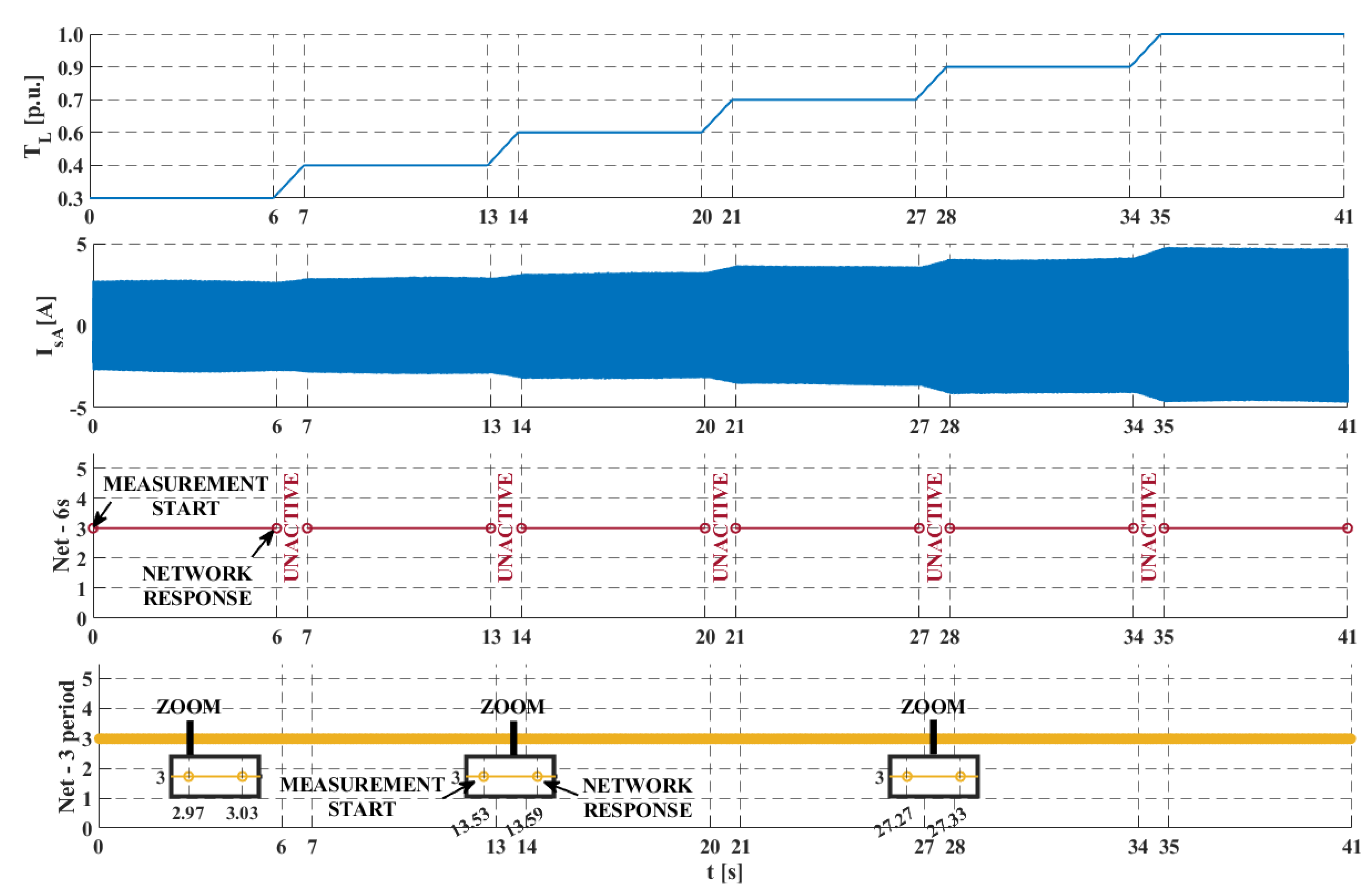
As a first test, it was decided to compare a network based on a full 6 s signal with a network based on the solution presented in the previous chapter using only three signal periods. The networks were compared for all the values of torque loads and fault types analyzed, and the example results are shown in
Figure 9. The first system mentioned shows a very good damage classification capability. Regardless of the value of the load, the system is able in the activity phases not only to diagnose the occurrence of damage but also to classify it accordingly. Unfortunately, the network can take as long as 6 s to collect data and determine the degree of damage. This presents some diagnostic problems as 6 s in the case of motor short circuits is a long acquisition time, during which serious and progressive insulation damage can occur. It can lead to complete inoperability of the motor, significantly increasing the cost of repairing such a motor or making such a repair completely impossible. A major issue is also the need to maintain the test object in a steady state, which is not a problem under laboratory conditions but is a major challenge under conditions of engine use such as in electromobility. Another limitation may also be the occurrence of cyclic short circuits (caused by incomplete insulation damage or by the mechanical design of the motor). These can have high values and cause rapid damage progression, but, due to their infrequent occurrence during the 6 s of measurement, they can be missed during signal processing, leading to a false damage classification. An additional difficulty, also highlighted in
Figure 9, is the inactivity of a system based on such a long measurement during transients. These locations are marked in
Figure 9 as inactive states. As already mentioned, under laboratory conditions, the maintenance of the selected conditions is not a problem, but, for motor applications in solutions such as electromobility, the motor may never reach a steady state, not to mention maintaining it for 6 s.
The second system presented, based on three measurement periods, also shows a high ability to classify faults, regardless of the value or state of the load (whether transient or steady). The system is also characterized by a very short reaction time to the occurring fault. Such a short response time not only allows rapid countermeasures to be taken in the event of a fault but also allows the response of the system to be averaged over several collected outputs to increase system confidence, avoiding false alarms caused by measurement noise or numerical errors. False diagnoses of damage can involve unnecessary shutdown of the facility, generating unnecessary costs (specialist work on diagnosing the object and downtime). An important advantage of the proposed system is its capability to perform accurate classification under transient operating conditions. Since only 600 signal samples are used for classification—corresponding to approximately three signal periods—the signal characteristics remain sufficiently stationary during the analysis window. Consequently, frequency-domain analysis using Fast Fourier Transform (FFT), typically restricted to steady-state signals, can still be effectively applied.
Both systems correctly classify damage, but, due to the time and operation conditions, the system based on three measurement periods is by far the better one to use for diagnostic purposes. It introduces the possibility of averaging the response, increasing its reliability, and does not show any problems working in a transient operation. Further analysis includes an investigation of the transient performance of this system for different natures of loads, for which the results are shown in
Figure 10,
Figure 11 and
Figure 12.
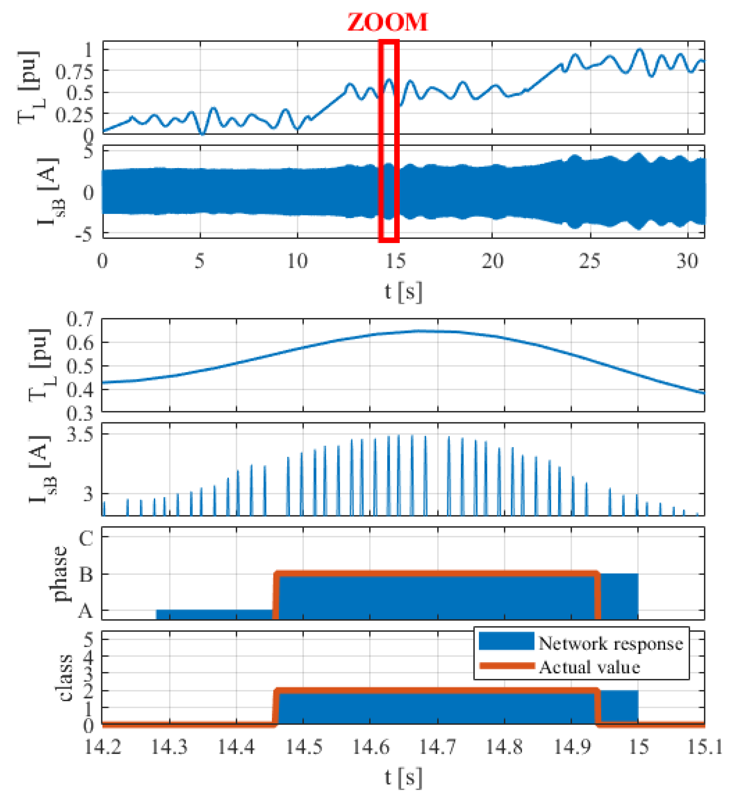
The experimental results show a selection of the response locations of the system for different loads to analyze its behavior in the case of fault diagnosis. The approximations were chosen to be presented because of the high accuracy of the network in general operation, which, with more than 30 s of measurement, makes it impossible to read the details of the reaction of the system in the case of short-circuit detection. To maintain the system verification credibility, different degrees and phases of faults and different load characteristics were tested. Zooms also show the connection points of the collected samples as sinusoidal-shape anomalies. This is due to the introduction of 50 break samples to check the correct operation of the system for samples starting at different phases and values (where the acquisition of three periods each time would result in data being collected at the same point in phase).
Figure 10 shows the performance of the system for a sawtooth load for the smallest degree of damage in phase A. The observed load change is close to 40%, but this did not prevent perfect fault diagnosis and classification. It is also worth noting that, when the signal returned to the no-damage state, the network did not sustain a response but continued to correctly classify the signal as undamaged. In
Figure 11, the performance of the system is presented for a random load within a certain range for two shorted coils in phase B, indicating that load fluctuation during the short circuit did not prevent the system from responding appropriately to the emerging fault, which was immediately classified accordingly. A problem did, however, arise with the return to the no-fault state, where the network sustained a fault condition for a further 0.06 s (one measurement sample). However, it can be seen that, after one response, the network returns to the no-fault state again, so the short sustained response can be attributed to the response averaging used.
To increase system confidence and reduce false alarms caused by measurement noise or numerical errors, the final classification is averaged over several collected outputs. This averaging, performed as a simple mean, results in a smoothed response during rapid changes in the actual fault condition. For example, during a transition from an undamaged state to a fault with three shorted turns, the initial averaged responses might indicate a lower damage degree (e.g., class 1 or 2). Conversely, when transitioning from a faulted state (e.g., three shorted turns) back to an undamaged state, the averaged response will show a similar gradual decrease rather than an instantaneous drop. While this contributes to the network not perfectly coinciding with the instantaneous actual waveform, it significantly enhances the reliability and stability of the system in practical diagnostic applications.
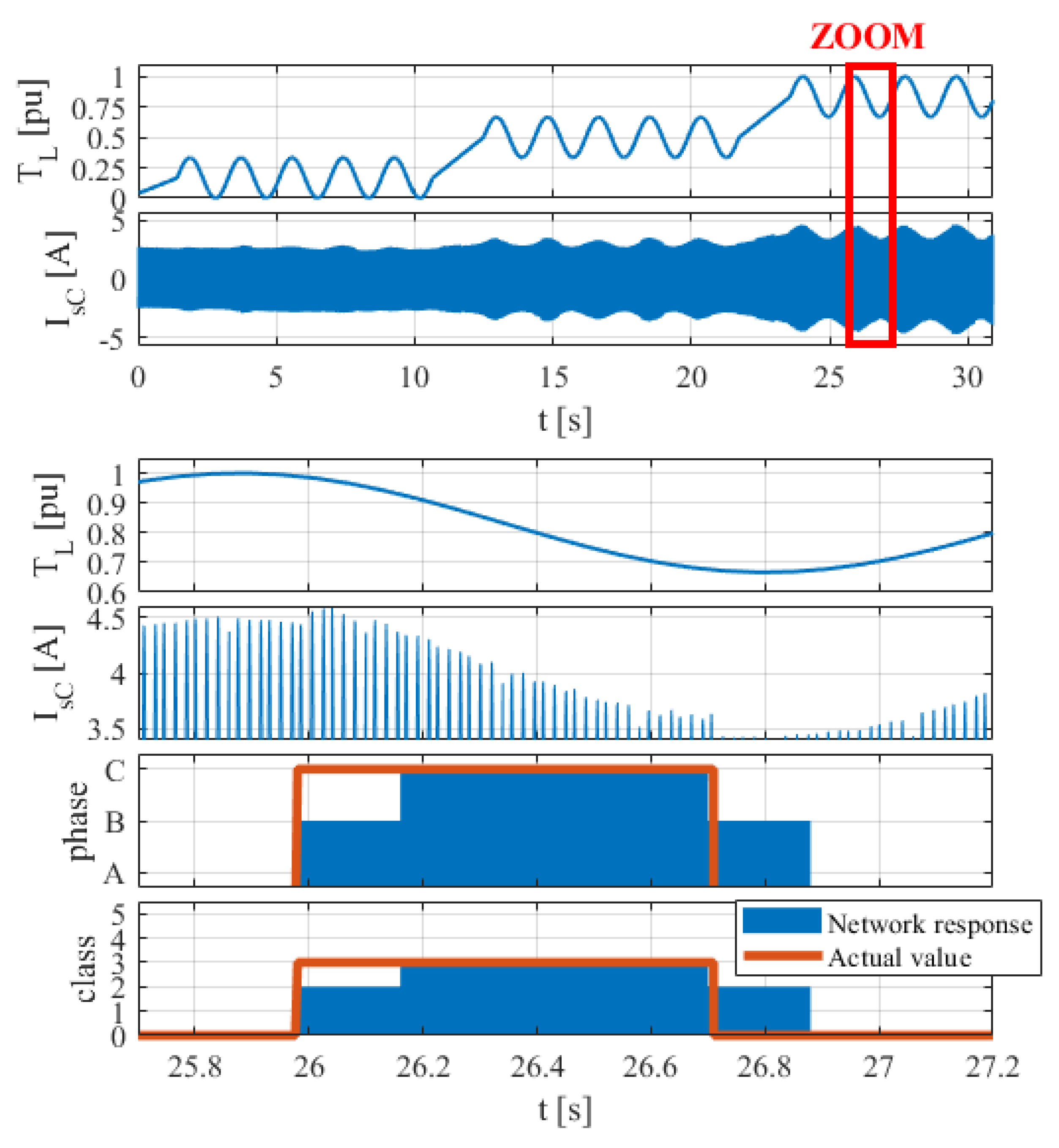
Moreover, the same reaction is observed for sinusoidal load variations (
Figure 12) for three shorted coils in phase C. The network response in this case does not perfectly coincide with the actual waveform of the modelled damage, but it can be seen that this may also be due to response averaging. However, despite the lack of a correct classification from the outset, it should be noted that damage was detected. In addition, a sustained response similar to that in
Figure 11 can be observed, but, due to the averaging of the result for damage value 3 and the subsequent undamaged state (denoted as 0), the averaging resulted in a lower damage degree being returned for the two measurement samples. After this, the system again appropriately indicates the undamaged state, which, due to the very short running time of the entire system (where the largest factor is the measurement time, i.e., 0.06 s), does not significantly affect the results.
7. Conclusions
The paper presents an innovative approach that combines classical signal processing techniques with both shallow and CNN architectures for the extraction and classification of fault symptoms in induction motors. The proposed system was designed to detect stator winding faults under both steady-state and transient operating conditions using a data buffer limited to only 600 signal samples—equivalent to approximately three fundamental periods. This short analysis window ensures that the signal remains sufficiently stationary, allowing effective application of frequency-domain methods such as Fast Fourier Transform (FFT), which are typically constrained to steady-state conditions. This represents a key advantage of the proposed method as it enables accurate diagnosis even during dynamic operating states. Although the current validation focuses specifically on turn short circuits, the fundamental approach could potentially be extended to other winding fault types, such as phase-to-phase or coil-to-ground faults, in future research. A comparative analysis with the classical approach [
39,
40] demonstrated that the proposed system achieved higher classification accuracy while significantly reducing the required data length and computational complexity. As such, the developed method offers a robust and efficient alternative to traditional diagnostic techniques based on time-domain, frequency-domain, or higher-order signal analysis.
The approach involved three levels of diagnostic information processing and was designed to ensure high precision in severity assessment and localization. At a 10 kHz sampling frequency, with the buffer mentioned above, direct application of spectral analysis was not feasible, which further excluded the use of Discrete Fourier Transform. The developed algorithm uses an SOM. This was despite the low spectral resolution caused by the limited number of samples and high sampling frequency. However, the analysis based solely on activated neurons allowed only for general fault detection. Therefore, matrix analysis using Euclidean distance measures was introduced via convolutional layers. A key distinction from traditional deep learning is its use of only a single convolutional layer. In this method, the CNN acts as a digital filter, shaping a feature space based on the Euclidean distance matrices.
The deep-learning-based diagnostic methods described in the literature typically require large training datasets and extensive computationally expensive training, often impractical in real-world implementations. The proposed technique is focused on delivering high accuracy when the available training dataset is limited. This also positions it as a viable alternative to transfer learning approaches, which still require comprehensive training datasets or accurate mathematical models. Fault characteristic knowledge was transferred between phases as the SOM training was based solely on measurements from phase A, eliminating the need to train a separate SOM for each stator phase. This was possible due to the analogous progression of faults in different motor phases and the resulting symptom correlation. The algorithm can serve as an alternative to neural diagnostic systems.
Author Contributions
Conceptualization, J.J.J. and M.S.; methodology, J.J.J. and M.S.; software, J.J.J. and M.S.; validation, J.J.J., M.S., O.F., M.W., S.W., J.V. and K.S.; visualization, O.F.; data curation, O.F. and M.W.; formal analysis, S.W., J.V., M.W. and K.S.; writing—original draft preparation, J.J.J., M.S. and O.F.; writing—review and editing, J.J.J., M.S., O.F., M.W., S.W., J.V. and K.S.; project administration, S.W. and K.S. All authors have read and agreed to the published version of the manuscript.
Funding
This research was funded by the European Union under GA no 101101961—HECATE. The views and opinions expressed are, however, those of the author(s) only, and do not necessarily reflect those of the European Union or the Clean Aviation Joint Undertaking. Neither the European Union nor the granting authority can be held responsible for them. This project is supported by the Clean Aviation Joint Undertaking and its Members.
Data Availability Statement
Data are contained within the article.
Conflicts of Interest
Authors Sebastien Weisse and Jerome Valire were employed by the company SAFRAN Electrical & Power. The remaining authors declare that the research was conducted in the absence of any commercial or financial relationships that could be construed as potential conflicts of interest.
Appendix A. Motor and Neural Network Specification Tables
Table A1.
Specifications of the Indukta Sh90L-4 IE1 induction motor used in the tests.
Table A1.
Specifications of the Indukta Sh90L-4 IE1 induction motor used in the tests.
| Parameter | Value |
|---|
| [kW] | 1.5 |
| [V] | 230 |
| [A] | 6.1 |
| n [rpm] | 1410 |
| T [N] | 10.16 |
| Number of poles | 4 |
| [Hz] | 50 |
| (number of rotor bars) | 26 |
| (number of stator turns in each phase) | 312 |
Table A2.
Specifications of the Kohonen network and its training hyperparameters used in the tests.
Table A2.
Specifications of the Kohonen network and its training hyperparameters used in the tests.
| Hyperparameter | Value |
|---|
| Map Size | 20 × 20 |
| Initial Learning Rate | 1 |
| Epochs | 10,000 |
| Initial Neighborhood Size | 10 |
| Neighborhood Function | Gaussian |
| Training Algorithm | Winner Takes Most |
Table A3.
Specifications of the CNN used in the tests.
Table A3.
Specifications of the CNN used in the tests.
| Layer | Parameters |
|---|
| Convolutional Layer | 10 filters 3 × 3 size |
| Normalization Layer | |
| Max Pooling Layer | 3 × 3 window size |
| Tanh Activation Layer | |
| Dropout Layer | probability 0.5 |
| Fully Connected Layer | output size 24 |
| Fully Connected Layer | output size 6 |
| Softmax Layer | |
Table A4.
Specifications of the CNN training used in the tests.
Table A4.
Specifications of the CNN training used in the tests.
| Hyperparameter | Value |
|---|
| Training algorithm | SGDM |
| Momentum | 0.9 |
| Initial Learning Rate | 0.005 |
| Epochs | 10,000 |
| Learn Rate Drop Schedule | ‘piecewise’ |
| Learn Rate Drop Factor | 0.95 |
| Learn Rate Drop Period | 20 |
| Mini-Batch Size | 8 |
| Regularization | L2 |
| Loss function | Cross-entropy |
References
- Krzysztofiak, M.; Zawilak, T.; Tarchała, G. Online control signal-based diagnosis of interturn short circuits of PMSM drive. Arch. Electr. Eng. 2023, 72, 103–124. [Google Scholar]
- Skowron, M.; Frankiewicz, O.; Jarosz, J.J.; Wolkiewicz, M.; Dybkowski, M.; Weisse, S.; Valire, J.; Wyłomańska, A.; Zimroz, R.; Szabat, K. Detection and Classification of Rolling Bearing Defects Using Direct Signal Processing with Deep Convolutional Neural Network. Electronics 2024, 13, 1722. [Google Scholar] [CrossRef]
- Skowron, M.; Oliszewski, S.; Dybkowski, M.; Jarosz, J.J.; Pawlak, M.; Weisse, S.; Valire, J.; Wyłomańska, A.; Zimroz, R.; Szabat, K. Applications of the TL-Based Fault Diagnostic System for the Capacitor in Hybrid Aircraft. Electronics 2024, 13, 1638. [Google Scholar] [CrossRef]
- Skowron, M.; Kowalski, C.T. Permanent magnet synchronous motor fault detection system based on transfer learning method. In Proceedings of the IECON 2022—48th Annual Conference of the IEEE Industrial Electronics Society, Brussels, Belgium, 17–20 October 2022; pp. 1–6. [Google Scholar]
- Kao, I.-H.; Wang, W.-J.; Lai, Y.-H.; Perng, J.-W. Analysis of permanent magnet synchronous motor fault diagnosis based on learning. IEEE Trans. Instrum. Meas. 2018, 68, 310–324. [Google Scholar] [CrossRef]
- Prieto, M.D.; Cirrincione, G.; Espinosa, A.G.; Ortega, J.A.; Henao, H. Bearing fault detection by a novel condition-monitoring scheme based on statistical-time features and neural networks. IEEE Trans. Ind. Electron. 2012, 60, 3398–3407. [Google Scholar] [CrossRef]
- Filippetti, F.; Franceschini, G.; Tassoni, C.; Vas, P. Recent developments of induction motor drives fault diagnosis using AI techniques. IEEE Trans. Ind. Electron. 2000, 47, 994–1004. [Google Scholar] [CrossRef]
- Tandon, N. A comparison of some vibration parameters for the condition monitoring of rolling element bearings. Measurement 1994, 12, 285–289. [Google Scholar] [CrossRef]
- Sarikhani, A.; Mohammed, O.A. Inter-turn fault detection in PM synchronous machines by physics-based back electromotive force estimation. IEEE Trans. Ind. Electron. 2012, 60, 3472–3484. [Google Scholar] [CrossRef]
- Leboeuf, N.; Boileau, T.; Nahid-Mobarakeh, B.; Clerc, G.; Meibody-Tabar, F. Real-time detection of interturn faults in PM drives using back-EMF estimation and residual analysis. IEEE Trans. Ind. Appl. 2011, 47, 2402–2412. [Google Scholar] [CrossRef]
- Minaz, M.R. An effective method for detection of stator fault in PMSM with 1D-LBP. ISA Trans. 2020, 106, 283–292. [Google Scholar] [CrossRef]
- Jung, J.-H.; Lee, J.-J.; Kwon, B.-H. Online diagnosis of induction motors using MCSA. IEEE Trans. Ind. Electron. 2006, 53, 1842–1852. [Google Scholar] [CrossRef]
- Thomson, W.T.; Fenger, M. Current signature analysis to detect induction motor faults. IEEE Ind. Appl. Mag. 2001, 7, 26–34. [Google Scholar]
- Ebrahimi, B.M.; Faiz, J. Feature extraction for short-circuit fault detection in permanent-magnet synchronous motors using stator-current monitoring. IEEE Trans. Power Electron. 2010, 25, 2673–2682. [Google Scholar]
- Haddad, R.Z.; Strangas, E.G. Fault detection and classification in permanent magnet synchronous machines using Fast Fourier Transform and Linear Discriminant Analysis. In Proceedings of the 2013 9th IEEE International Symposium on Diagnostics for Electric Machines, Power Electronics and Drives (SDEMPED), Valencia, Spain, 27–30 August 2013; pp. 99–104. [Google Scholar]
- Bouzida, A.; Touhami, O.; Ibtiouen, R.; Belouchrani, A.; Fadel, M.; Rezzoug, A. Fault diagnosis in industrial induction machines through discrete wavelet transform. IEEE Trans. Ind. Electron. 2010, 58, 4385–4395. [Google Scholar] [CrossRef]
- Pons-Llinares, J.; Antonino-Daviu, J.A.; Riera-Guasp, M.; Lee, S.B.; Kang, T.-j.; Yang, C. Advanced induction motor rotor fault diagnosis via continuous and discrete time–frequency tools. IEEE Trans. Ind. Electron. 2014, 62, 1791–1802. [Google Scholar] [CrossRef]
- Fang, J.; Sun, Y.; Wang, Y.; Wei, B.; Hang, J. Improved ZSVC-based fault detection technique for incipient stage inter-turn fault in PMSM. IET Electr. Power Appl. 2019, 13, 2015–2026. [Google Scholar]
- Urresty, J.-C.; Riba, J.-R.; Saavedra, H.; Romeral, L. Detection of inter-turns short circuits in permanent magnet synchronous motors operating under transient conditions by means of the zero sequence voltage. In Proceedings of the 2011 14th European Conference on Power Electronics and Applications, Birmingham, UK, 30 August–1 September 2011; pp. 1–9. [Google Scholar]
- Bazan, G.H.; Scalassara, P.R.; Endo, W.; Goedtel, A.; Palácios, R.H.C.; Godoy, W.F. Stator short-circuit diagnosis in induction motors using mutual information and intelligent systems. IEEE Trans. Ind. Electron. 2018, 66, 3237–3246. [Google Scholar]
- Ghate, V.N.; Dudul, S.V. Optimal MLP neural network classifier for fault detection of three phase induction motor. Expert Syst. Appl. 2010, 37, 3468–3481. [Google Scholar]
- Germen, E.; Başaran, M.; Fidan, M. Sound based induction motor fault diagnosis using Kohonen self-organizing map. Mech. Syst. Signal Process. 2014, 46, 45–58. [Google Scholar]
- Saucedo-Dorantes, J.J.; Jaen-Cuellar, A.Y.; Perez-Cruz, A.; Elvira-Ortiz, D.A. Detection of Inter-Turn Short Circuits in Induction Motors under the Start-Up Transient by Means of an Empirical Wavelet Transform and Self-Organizing Map. Machines 2023, 11, 958. [Google Scholar] [CrossRef]
- Srinivasan, A.; Batur, C. Hopfield/ART-1 neural network-based fault detection and isolation. IEEE Trans. Neural Netw. 1994, 5, 890–899. [Google Scholar] [CrossRef] [PubMed]
- Skowron, M. Development of a universal diagnostic system for stator winding faults of induction motor and PMSM based on transfer learning. In Proceedings of the 2023 IEEE 14th International Symposium on Diagnostics for Electrical Machines, Power Electronics and Drives (SDEMPED), Chania, Greece, 28–31 August 2023; pp. 517–523. [Google Scholar]
- Luo, Y.; Qiu, J.; Shi, C. Fault detection of permanent magnet synchronous motor based on deep learning method. In Proceedings of the 2018 21st International Conference on Electrical Machines and Systems (ICEMS), Jeju, Republic of Korea, 7–10 October 2018; pp. 699–703. [Google Scholar]
- Yang, Z.; Huang, Y.; Nazeer, F.; Zi, Y.; Valentino, G.; Li, C.; Long, J.; Huang, H. A novel fault detection method for rotating machinery based on self-supervised contrastive representations. Comput. Ind. 2023, 147, 103878. [Google Scholar] [CrossRef]
- Kim, M.; Jung, J.H.; Ko, J.U.; Kong, H.B.; Lee, J.; Youn, B.D. Direct connection-based convolutional neural network (DC-CNN) for fault diagnosis of rotor systems. IEEE Access 2020, 8, 172043–172056. [Google Scholar] [CrossRef]
- Wen, L.; Li, X.; Gao, L.; Zhang, Y. A new convolutional neural network-based data-driven fault diagnosis method. IEEE Trans. Ind. Electron. 2017, 65, 5990–5998. [Google Scholar] [CrossRef]
- Shao, S.; McAleer, S.; Yan, R.; Baldi, P. Highly accurate machine fault diagnosis using deep transfer learning. IEEE Trans. Ind. Inf. 2018, 15, 2446–2455. [Google Scholar]
- Yang, B.; Lei, Y.; Jia, F.; Xing, S. An intelligent fault diagnosis approach based on transfer learning from laboratory bearings to locomotive bearings. Mech. Syst. Signal Process. 2019, 122, 692–706. [Google Scholar] [CrossRef]
- Kliman, G.B.; Stein, J. Methods of motor current signature analysis. Electr. Mach. Power Syst. 1992, 20, 463–474. [Google Scholar] [CrossRef]
- Benbouzid, M.E.H. A review of induction motors signature analysis as a medium for faults detection. IEEE Trans. Ind. Electron. 2000, 47, 984–993. [Google Scholar] [CrossRef]
- Thomson, W.T.; Barbour, A. On-line current monitoring and application of a finite element method to predict the level of static airgap eccentricity in three-phase induction motors. IEEE Trans. Energy Convers. 1998, 13, 347–357. [Google Scholar] [CrossRef]
- Skowron, M.; Wolkiewicz, M.; Orlowska-Kowalska, T.; Kowalski, C.T. Application of self-organizing neural networks to electrical fault classification in induction motors. Appl. Sci. 2019, 9, 616. [Google Scholar] [CrossRef]
- Das, A.K.; Das, S.; Pradhan, A.K.; Chatterjee, B.; Dalai, S. RPCNNet: A Deep Learning Approach to Sense Minor Stator Winding Interturn Fault Severity in Induction Motor Under Variable Load Condition. IEEE Sensors J. 2023, 23, 3965–3972. [Google Scholar] [CrossRef]
- Husari, F.; Seshadrinath, J. Stator Turn Fault Diagnosis and Severity Assessment in Converter-Fed Induction Motor Using Flat Diagnosis Structure Based on Deep Learning Approach. IEEE J. Emerg. Sel. Top. Power Electron. 2023, 11, 5649–5657. [Google Scholar] [CrossRef]
- Min, T.-H.; Lee, J.-H.; Choi, B.-K. CNN-Based Fault Classification in Induction Motors Using Feature Vector Images of Symmetrical Components. Electronics 2025, 14, 1679. [Google Scholar] [CrossRef]
- Coelho, D.N.; Barreto, G.A.; Medeiros, C.M.S. Detection of Short Circuit Faults in 3-Phase Converter-Fed Induction Motors Using Kernel SOMs. In Proceedings of the 2017 12th International Workshop on Self-Organizing Maps and Learning Vector Quantization, Clustering and Data Visualization (WSOM), Salamanca, Spain, 27–29 June 2017; pp. 1–6. [Google Scholar]
- Ofosu, R.A.; Odoi, B.; Boateng, D.F.; Muhia, A.M. Fault Detection and Diagnosis of a 3-Phase Induction Motor Using Kohonen Self-Organising Map. J. Nas. Tek. Elektro 2023, 12, 31–41. [Google Scholar] [CrossRef]
| Disclaimer/Publisher’s Note: The statements, opinions and data contained in all publications are solely those of the individual author(s) and contributor(s) and not of MDPI and/or the editor(s). MDPI and/or the editor(s) disclaim responsibility for any injury to people or property resulting from any ideas, methods, instructions or products referred to in the content. |
© 2025 by the authors. Licensee MDPI, Basel, Switzerland. This article is an open access article distributed under the terms and conditions of the Creative Commons Attribution (CC BY) license (https://creativecommons.org/licenses/by/4.0/).


 ,
, 


