Elevator Fault Diagnosis Based on a Graph Attention Recurrent Network

Abstract

Elevator fault diagnosis is critical for ensuring operational safety and reliability in modern vertical transportation systems. Traditional approaches, which rely on time- and frequency-domain signal analysis, often struggle with the issues such as noise sensitivity, inadequate feature extraction, and limited adaptability to complex scenarios. To address these challenges, this paper proposes a Graph Attention Recurrent Network (GARN) which integrates graph-structured signal representation with spatiotemporal feature learning. The GARN employs a limited penetrable visibility graph to transform raw vibration signals into noise-robust graph topologies, preserving critical patterns while suppressing high-frequency noise through controlled edge penetration. An adaptive attention mechanism dynamically fuses triaxial features to prioritize the most relevant information for fault diagnosis. The GARN combines a graph convolutional network to extract spatial correlations and a gated recurrent unit to capture temporal fault progression, enabling holistic and accurate fault classification. Experimental results based on real-world elevator datasets demonstrate the superior performance of the GARN, showcasing its strong noise resistance, adaptability to complex fault conditions, and ability to provide reliable and timely fault diagnosis, making it a robust solution for modern elevator systems.

1. Introduction

Elevators are essential to the infrastructure of smart buildings and play a crucial role in urban transportation, moving millions of people daily. The reliability and safety of elevators directly impact the quality of life in cities. Enhancing elevator safety is a primary concern, as failures in critical components can lead to serious accidents, endangering both passengers and maintenance personnel. With the increasing number of elevators, ensuring their safety and reliability becomes more challenging.

Traditional maintenance paradigms for elevator systems, including time-based maintenance and corrective maintenance strategies, remain predicated upon standardized schedules and human-dependent inspection protocols. Time-based maintenance assesses components at fixed intervals, ignoring operational degradation. Corrective maintenance protocols exhibit greater passivity, initiating interventions exclusively post-failure, with consequent operational disruptions and elevated repair expenditures. Both methodologies necessitate substantial technician deployment, demonstrating inherent inefficiencies in labor utilization and temporal requirements while proving inadequate for addressing the heterogeneous operational demands characteristic of contemporary vertical transportation infrastructure.

In contrast, the condition-based maintenance strategy emphasizes the continuous monitoring of vibration in components exhibiting signs of wear or damage. For elevators, condition-based maintenance primarily relies on the analysis of vibration signals in both the time and frequency domains. These approaches integrate advanced signal processing techniques with machine learning models, such as multilayer perceptrons, support vector machines, and Bayesian estimation, to identify faults characterized by clear and distinguishable patterns. Recent developments in adaptive control frameworks, as demonstrated by Zhang et al. [1] through their siphon-based supervisory policy for unreliable-resource management in automated manufacturing systems, suggest potential extensions for maintenance strategies. Their methodology dynamically adjusts system modes to accommodate component failures while preserving original operational behavior, a concept that could inform adaptive maintenance policy design for elevator systems with heterogeneous component degradation patterns. For example, wavelet denoising proves effective in removing noise from horizontal vibration signals, thereby revealing irregularities in the guide rail that compromise ride comfort. The denoised signals, with their enhanced features, enable precise localization of guide rail faults [2]. Similarly, autoregressive models utilize autoregressive coefficients derived from processed signals as inputs for support vector machines, facilitating automated fault recognition [3]. Furthermore, a bicoherence-based method is proposed for elevator fault diagnosis, leveraging autoregressive modeling to capture nonlinear couplings and mitigate the impact of Gaussian noise in vibration signals [4]. These techniques collectively enhance the accuracy and reliability of fault detection in elevator systems.

While demonstrating diagnostic competence for elementary fault patterns, extant vibration analysis methodologies exhibit three principal constraints when confronting multifactorial failure modes that are prevalent in modern elevator ecosystems. First, the dependency on manual time–frequency feature engineering introduces significant noise susceptibility, particularly in operational environments characterized by non-stationary disturbances. Although wavelet thresholding proves effective in controlled conditions, empirical studies reveal substantial performance degradation under high-noise scenarios, due to transient feature attenuation. Second, conventional machine learning architectures (e.g., support vector machines, Bayesian classifiers) demonstrate limited capacity for modeling nonlinear signal interactions and cross-scale dependencies, constraining generalizability across diverse failure modalities. Third, prevailing analytical frameworks predominantly analyze uniaxial vibration data, thereby neglecting the diagnostic potential inherent in triaxial signal correlations, which are critical for differentiating spectrally analogous but spatially distinct fault signatures. These limitations collectively underscore the necessity of advanced analytical frameworks that are capable of processing multidimensional vibration data through deep feature learning architectures.

The advent of neural networks has introduced new possibilities in vibration-based fault diagnosis. Deep autoencoders can be employed to extract meaningful features from raw sensor data, enabling effective fault classification [5]. Additionally, the wavelet packet decomposition method, combined with neural networks, has proven effective in distinguishing normal and faulty states within noisy vibration signals [6]. Deep learning algorithms revolutionize fault diagnosis with their superior feature extraction and pattern recognition capabilities. Architectures such as convolutional neural networks, autoencoders, and generative adversarial networks are used to diagnose complex mechanical faults [7,8,9,10,11]. For instance, one-dimensional convolutional neural networks can be employed to extract features and achieve high diagnostic accuracy, particularly in scenarios characterized by limited sample sizes [12]. A deep wavelet autoencoder, combined with extreme learning machines, demonstrated effectiveness in diagnosing rolling bearing faults by capturing both time-domain and frequency-domain characteristics [13].

Currently, deep learning techniques such as one-dimensional convolutional neural networks, Deep Boltzmann Machines, and transfer learning show promise in fault diagnosis, particularly for bearing failures. However, these methods face significant challenges when applied to elevator fault diagnosis. The primary obstacles include the need for large datasets, which are often unavailable in elevator systems, leading to insufficient training data. Additionally, issues such as poor feature interpretability and unstable performance in small-sample scenarios hinder their effectiveness. As a result, these methods struggle to handle the complexities and diversity of elevator fault conditions, limiting their broader applicability.

Graph neural networks have been successfully applied in various domains, including social networks, natural language processing, and fault diagnosis [14,15,16,17,18]. Recent advances in graph structure learning, such as Neural Gaussian Similarity Modeling [19], have further enhanced noise-resilient edge formation through differentiable sampling strategies, complementing domain-specific approaches like LPVG. Graph neural networks leverage their ability to model relational data and capture structural dependencies to improve troubleshooting capabilities. Methods like gradient-based interpretable graph convolutional networks (GCNs) further improve model transparency in diagnosing bearing faults.

The integration of multi-view information, as proposed in mutual information maximization across feature and topology views [20], aligns with GARNs’ attention-driven fusion of triaxial vibration data, where directional dependencies are dynamically weighted to prioritize diagnostically critical axes. Multivariate anomaly detection with a self-learning GCN effectively captures spatial and temporal correlations within input sequences [21]. Another study uses the k-nearest neighbor method to construct graphs to establish relationships, thus providing efficient feature extraction for GCN fault classification [22]. Recent research focuses on multidimensional, multi-scale, and multi-channel data for fault diagnosis. For multi-channel graph analysis, the cross-channel information bottleneck principle (CCGIB) [23] provides a theoretical foundation for balancing consistency and complementarity in sensor fusion, a challenge directly addressed by GARNs’ adaptive attention mechanism. Multi-scale GCNs and improved multi-channel GCNs process data from multiple sensors, capturing complex fault features [24,25]. For temporal data, transforming time-series data into graph structures, such as weighted horizontal visibility graphs, proves effective in capturing both local and global signal features. The improved graph isomorphism network has shown promising results in fault classification tasks [26]. Similarly, while graph neural networks garner attention for their ability to process non-Euclidean relational data, their current application is largely focused on bearing fault diagnosis. This makes it challenging to adapt existing graph neural networks methods to the specific dynamics of elevator faults. Despite graph neural networks’ potential to model relational data and capture structural dependencies, the lack of research directly addressing elevator systems means that these models struggle to effectively capture the nuances of elevator fault behaviors. Consequently, current deep learning and graph neural network-based methods are limited in their ability to address the unique complexities of elevator fault diagnosis, highlighting the need for further advancements tailored to this domain.

Elevator fault diagnosis faces several significant challenges that hinder the effectiveness and broader applicability of existing methods:

• The diversity and complexity of elevator systems make it difficult for traditional methods to effectively capture the wide range of fault conditions.
• A lack of labeled data, particularly for rare or complex faults, restricts the generalization ability of diagnostic models, leading to overfitting, especially when using deep neural networks.
• While graph neural networks have proven effective in handling relational data, they have not been widely tested for elevator fault diagnosis. Existing graph neural network methods are primarily focused on simpler systems, such as bearing fault diagnosis, which have less complex fault dynamics.
• Adapting graph neural networks to the unique complexities of elevator systems, with their dynamic operating states and diverse fault conditions, presents significant challenges.

To address these challenges, this paper proposes a Graph Attention Recurrent Network (GARN). The GARN framework introduces significant advancements and methodological innovations in addressing the challenges associated with elevator fault diagnosis. The key contributions and technical merits of the approach are outlined below:

• Enhanced Noise Tolerance by Limited Penetration Visibility Graph (LPVG) Conversion: A fundamental innovation of GARN is the incorporation of the LPVG method, which converts raw vibration signals into graph-based representations. The LPVG algorithm is specifically designed to mitigate the impact of noise during graph construction by permitting controlled penetration thresholds. This noise-tolerant mechanism is particularly advantageous in elevator environments, where vibration signals are often contaminated by extraneous noise, ensuring the preservation of diagnostic accuracy under adverse conditions.
• Spatial Feature Extraction via GCN: The GARN employs a GCN to extract spatial features from the graph-structured vibration data. The GCN architecture is uniquely suited to model the spatial dependencies and interrelationships among various nodes in the graph, thereby capturing the inherent structural patterns of the vibration signals. This capability is critical for identifying subtle fault signatures that may be distributed across different spatial regions of the signal.
• Attention-Driven Multi-Axis Data Fusion: The framework incorporates an attention-based mechanism to dynamically integrate features derived from the triaxial vibration data (x, y, and z axes). This mechanism assigns adaptive weights to each axis based on its diagnostic relevance, enabling the model to prioritize the most informative directional components. By selectively emphasizing critical features, the attention mechanism enhances the model’s ability to detect faults with diverse directional characteristics, thereby improving the overall classification accuracy and diagnostic precision.
• Temporal Modeling with Gated Recurrent Units (GRUs): To capture temporal dependencies within vibration signals, the GARN employs GRUs, which are well-suited for sequential data. The GRUs allow the model to track the evolution of fault signals over time, distinguishing between transient disturbances and ongoing fault conditions. This temporal modeling capability strengthens the framework’s ability to provide accurate and timely fault diagnoses in dynamic elevator systems.
• Modern elevator systems are increasingly embedded within IoT ecosystems, where sensor-generated data streams necessitate real-time, adaptive fault diagnosis frameworks. The proposed GARN architecture not only addresses the limitations of traditional methods, but also aligns with the demands of software-defined IoT environments, such as QoS (Quality of Service)-aware resource allocation and edge computing efficiency. For instance, in smart buildings leveraging QoS-aware IoT protocols, the GARN’s low-latency inference (0.01 s per sample) ensures timely fault alerts, minimizing operational disruptions. Furthermore, its compatibility with streaming data architectures—such as those in software-defined vehicular networks—positions it as a versatile solution for dynamic environments requiring rapid, multi-sensor analytics. By integrating graph-based spatiotemporal learning with IoT operational paradigms, this work bridges the gap between theoretical fault diagnosis and practical deployment in next-generation smart infrastructure.

The GARN delivers a solution for elevator fault diagnosis in complex scenarios. The remainder of this paper is structured as follows: Section 2 describes the GARN in detail; Section 3 outlines the dataset used for validation; Section 4 discusses the experiments and results; and we conclude the study in Section 5.

2. The Proposed Method

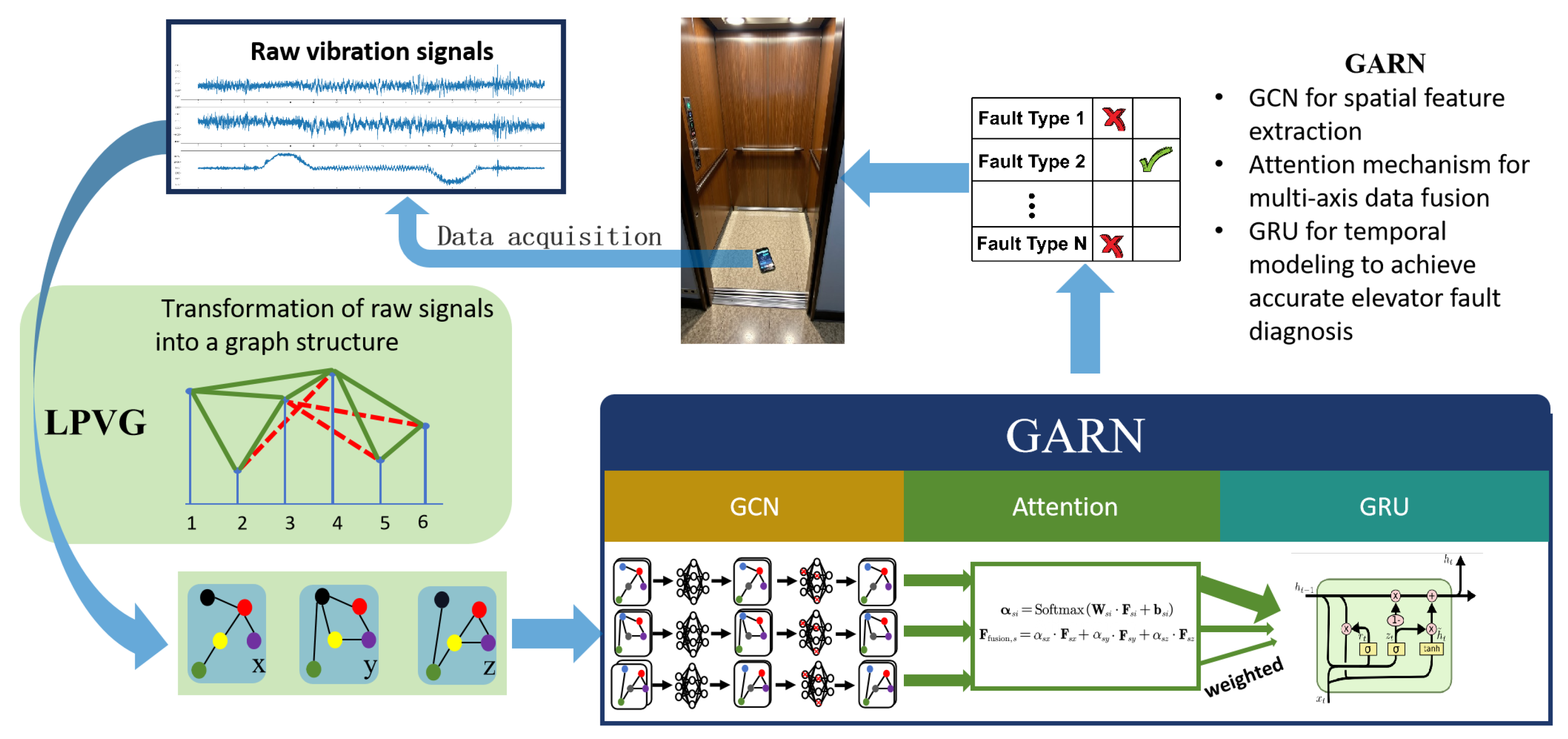
To tackle the challenges of noise resilience, multi-axis data integration, and temporal feature modeling in elevator fault diagnosis, we propose a novel diagnostic framework. As shown in Figure 1, the GARN involves several key steps:

• First, in the data preprocessing phase, raw vibration signals collected from the x, y, and z axes are subjected to a sliding-window technique. This technique segments the original data into sequences.
• Next, these segmented sequences are transformed into graph representations using the LPVG method. This transformation captures both the temporal and structural patterns of the data and enhances noise immunity.
• The GCN is then employed to learn meaningful representations from the graph-structured data by aggregating and propagating information across nodes and their neighbors. An attention-based fusion mechanism is incorporated to dynamically integrate features extracted from the three axes. This mechanism assigns adaptive weights to each axis, prioritizing the most relevant directional information for fault diagnosis.
• Finally, the fused features are processed by a GRU network, which captures temporal dependencies in the vibration signals, enabling accurate and efficient fault classification.

Figure 1. Graph attention recurrent network.

Figure 1. Graph attention recurrent network.

The vibration time-series dataset of an axis is $X=\langle x_1,x_2,\dots ,x_N\rangle$, where N denotes the number of samples, and the sliding window method is applied to divide X into windows of length L, with a step size of $\eta$. The number of windows n is determined by $n={\displaystyle \frac{N}{\eta }}$. The index of the window is s, which ranges from 1 to n. Each segment $X_s=\langle x_{s1},x_{s2},\dots ,x_{sL}\rangle$ corresponds to a window, and each window is transformed into a graph representation $G_s=(V_s,E_s)$ using the LPVG method. The set of nodes is $V_s$ and the edges between nodes are $E_s$.

2.1. Graph Construction by LPVG

The LPVG is an extension of the visibility graph (VG), designed to improve noise immunity during graph construction. A VG, derived from computational geometry, is commonly used to represent visibility relationships among points in a sequence or plane. An edge is formed between two points if there exists an unobstructed path that satisfies the visibility condition.

The LPVG addresses the limitations of traditional visibility graphs (VGs). As illustrated in Figure 2, the LPVG systematically recovers edges that standard VG methods fail to detect under noisy conditions. This improvement stems from two key modifications: (1) flexible adaptation of visibility criteria and (2) implementation of distance-based edge constraints. By tolerating minor data fluctuations while maintaining core visibility principles, the LPVG achieves an enhanced structural representation of complex systems without sacrificing graph interpretability. The methodology demonstrates particular effectiveness in analyzing noisy dynamical systems, where conventional VGs produce fragmented connectivity patterns.

The LPVG approach enhances graphics with a manageable tolerance for visibility violations, permitting connections when up to $\delta$ intermediate points fail to meet standard visibility criteria. For any pair of nodes $x_{si}$ and $x_{sj}$ ($i<j$) within segment $X_s$, the edge formation follows the following mathematical constraints:

$$\begin{array}{c}\hfill x_{sk}<x_{si}+{\displaystyle \frac{x_{sj}-x_{si}}{j-i}}·(k-i),\\ \hfill \forall k\in \{i+1,\dots ,j-1\},\\ \hfill \forall s\in \{1,2,\dots ,N-L+1\},\end{array}$$

(1)

where $x_{sk}$ represents intermediate values between the candidate nodes. This criterion requires that the majority of points maintain linear visibility, with edge creation permitted when violating points ($N_{\mathrm{violate}}$) satisfy $N_{\mathrm{violate}}<\delta$. The parametric control through $\delta$ enables systematic adaptation to data irregularities while preserving essential topological relationships.

Depending on the presence or absence of edges between two points in the LPVG, each segment $X_s$ has then an adjacency matrix $A_s\in {\mathbb{R}}^{L\times L}$, where $A_{sij}=1$ if an edge exists between nodes $x_{si}$ and $x_{sj}$, and $A_{sij}=0$ otherwise.

2.2. LPVG Construction Steps

Given a raw one-dimensional vibration signal sequence $X=\{x_1,x_2,\dots ,x_N\}$, we first apply a sliding window to segment the signal into overlapping or non-overlapping subsequences. Let L denote the window length and $\eta$ denote the step size. The s-th segment is denoted as

$$X_s=\{x_{s1},x_{s2},\dots ,x_{sL}\},$$

(2)

where $x_{si}=x_{(s-1)\eta +i}$. Each segment $X_s$ will be transformed into a graph $G_s=(V_s,E_s)$ via the limited penetrable visibility graph (LPVG) method.

The graph construction follows the principle of visibility between time-series data points. Each point $x_{si}$ in the window becomes a node $v_i\in V_s$. The two nodes $v_i$ and $v_j$ (with $i<j$) are connected by an edge $e_{ij}\in E_s$ if the majority of the intermediate points do not obstruct the direct line of sight between $x_{si}$ and $x_{sj}$. Formally, the penetrable visibility condition is given as

$$x_{sk}<x_{si}+{\displaystyle \frac{x_{sj}-x_{si}}{j-i}}(k-i),\forall k\in \{i+1,\dots ,j-1\}\mathrm{with}\mathrm{at}\mathrm{most}\delta \mathrm{violations}.$$

(3)

This condition allows up to $\delta$ intermediate points $x_{sk}$ to violate the strict visibility criterion. If the number of violations is less than $\delta$, then an edge is established between nodes $v_i$ and $v_j$.

After evaluating all the possible pairs $(i,j)$ within each segment, we obtain a sparse adjacency matrix $A_s\in {\mathbb{R}}^{L\times L}$, where

$$A_{sij}=\left\{\begin{array}{cc}1,\hfill & \mathrm{if}\mathrm{edge}{e}_{ij}\mathrm{exists},\hfill \\ 0,\hfill & \mathrm{otherwise}.\hfill \end{array}\right.$$

(4)

This procedure is applied independently to each segment $X_s$ of the signal across all three vibration axes (x, y, z), yielding a sequence of graph-structured data. These LPVG graphs serve as robust structural encodings for the downstream graph neural network, where the limited penetrability ($\delta$) effectively suppresses transient noise while preserving the essential dynamical patterns.

2.3. Feature Extraction by GCN

The GCN extracts features from the graph structure. The GCN propagates information through graph layers by aggregating and transforming neighborhood information. A GCN is a class of neural networks specifically designed for graph-structured data. Unlike traditional convolutional neural networks, which operate on grid-like data such as images, a GCN leverages the relationships between nodes to update node features through message passing along the edges of the graph. This capability makes GCNs particularly effective for tasks such as node classification, link prediction, and graph classification.

A spatial GCN implements hierarchical learning through three core operations: localized aggregation, nonlinear feature fusion, and structural readout. The framework first propagates neighborhood features via message passing with learnable attention weights, subsequently combining transformed neighbor embeddings with ego-node representations through multilayer nonlinear transformations. Finally, graph-level pooling operators generate topology-aware embeddings by aggregating node features with permutation-invariant functions.

This architecture enables progressive encoding of local substructures and global connectivity patterns. Through iterative neighborhood aggregation, the spatial GCN demonstrates graph sparsity and noise while maintaining structural awareness, effectively balancing local detail preservation and global context integration in graph representation learning. For a graph with the node feature matrix $H^{\left(0\right)}\in {\mathbb{R}}^{L\times d}$, where d is the feature dimension, the layer-wise propagation rule of the GCN is

$$H^{(l+1)}=\sigma \left({\widetilde{D_s}}^{-1/2}\widetilde{A_s}{\widetilde{D_s}}^{-1/2}{H}^{\left(l\right)}{W}^{\left(l\right)}\right),$$

(5)

where $\widetilde{A_s}=A_s+I$ is the adjacency matrix, with I being the identity matrix; the matrix $\widetilde{D_s}$ denotes the degree of $\widetilde{A_s}$; the node features at the l-th layer are represented by $H^{\left(l\right)}$, with $H^{\left(0\right)}=X_s$ and $l=0,1,\dots ,L-1$; the trainable weight matrix of the l-th layer is denoted by $W^{\left(l\right)}$; and the nonlinear activation function is represented as $\sigma (·)$.

At each layer, the GCN aggregates information from the immediate neighbors of a node to update its feature representation. By stacking multiple GCN layers, the network progressively captures higher-order dependencies between nodes, allowing it to model increasingly complex neighborhood relationships and better capture the structural information inherent in the graph.

2.4. Feature Fusion by Attention Mechanism

For elevator fault diagnosis, three-axis vibration data plays a crucial role, as each axis captures distinct vibration directions with unique characteristics. The recorded vibration signals correspond to three axes: the x-axis, y-axis, and z-axis. The x-axis is oriented perpendicular to the elevator door, the y-axis is parallel to the door, and the z-axis is perpendicular to the ground.

To effectively combine the three-axis vibration data (x-axis, y-axis, and z-axis) and capture the most relevant directional information for elevator fault diagnosis, an attention mechanism is employed. This approach dynamically assigns different weights to each axis, highlighting the most informative features for the task.

The features extracted by the GCN from the x, y, and z axes of the vibration data are denoted as $F_{sx}$, $F_{sy}$, and $F_{sz}$, respectively. The attention mechanism computes weights for each axis based on their contributions. The attention network is used to determine the importance of the features from each axis. The attention score ${\alpha }_{si}$ for each axis $i\in \{x,y,z\}$ is calculated by

$$F_{si}=\mathrm{Softmax}\left(W_{si}·F_{si}+b_{si}\right),$$

(6)

where $W_{si}$ is a trainable weight vector for axis i, and $b_{si}$ is a bias term. The operator ‘·’ denotes matrix multiplication, and the function $\mathrm{Softmax}(·)$ ensures that the attention scores sum to 1 across the three axes.

The calculated attention weights ${\alpha }_{sx}$, ${\alpha }_{sy}$, and ${\alpha }_{sz}$ indicate the relative importance of features from the x, y, and z axes, respectively. The fused feature representation $F_{\mathrm{fusion},s}$ is computed as a weighted sum of the features from all three axes:

$$F_{\mathrm{fusion},s}={\alpha }_{sx}·F_{sx}+{\alpha }_{sy}·F_{sy}+{\alpha }_{sz}·F_{sz},$$

(7)

where ${\alpha }_{sx}$, ${\alpha }_{sy}$, and ${\alpha }_{sz}$ are the attention weights for the x, y, and z axes, and the symbol · denotes element-wise multiplication.

The fusion process employs axis-specific feature weighting to selectively amplify diagnostically relevant patterns in triaxial vibration data. By analyzing directional dependencies across sensor axes through trainable attention layers, the system automatically calibrates inter-axis contributions during feature integration. This adaptive weighting strategy produces composite representations, $F_{\mathrm{fusion},s}$, that maintain discriminative three-dimensional characteristics while suppressing redundant information, thereby preserving critical fault signatures that are essential for accurate classification.

2.5. Fault Diagnosis by GRUs

Following feature fusion, the temporal pattern analysis module employs GRUs to model sequential dependencies in elevator operational states. As a streamlined alternative to conventional LSTM architectures, GRUs maintain temporal modeling capabilities while optimizing computational efficiency through architectural simplification. The network’s dual regulatory components, which are the update gate ($z_s$) and the reset gate ($r_s$), implement dynamic information filtering by adaptively retaining critical historical states while discarding transient noise patterns.

The update gate controls how much of the previous hidden state $h_{s-1}$ is retained in the current hidden state $h_s$, calculated by

$$z_s=\sigma \left(W_z·F_{\mathrm{fusion},s}+U_z·h_{s-1}+b_z\right),$$

(8)

where $\sigma (·)$ is the sigmoid activation function. In the update gate, $W_z$ and $U_z$ are the weight matrices for the current input $F_{\mathrm{fusion},s}$. The symbol $b_z$ is the bias term. The reset gate determines how much of the previous hidden state should be ignored when calculating the candidate hidden state ${\tilde{h}}_s$, computed by

$$r_s=\sigma \left(W_r·F_{\mathrm{fusion},s}+U_r·h_{s-1}+b_r\right),$$

(9)

where $W_r$ and $U_r$ are the weight matrices of the reset gate and $b_r$ is the bias term. The candidate hidden state ${\tilde{h}}_s$ is computed based on the reset gate, which controls how much of the previous hidden state is reset, computed by

$${\tilde{h}}_s=tanh\left(W_h·F_{\mathrm{fusion},s}+U_h·(r_s\odot h_{s-1})+b_h\right),$$

(10)

where $tanh(·)$ is the hyperbolic tangent activation function, and the element-wise multiplication is denoted as ⊙. The weight matrices are $W_h$ and $U_h$. The bias term is $b_h$.

The final hidden state $h_s$ is computed by combining the previous hidden state and the candidate hidden state, controlled by the update gate. It is updated by following equation:

$$h_s=z_s\odot h_{s-1}+(1-z_s)\odot {\tilde{h}}_s.$$

(11)

This hidden state $h_s$ contains information from both the previous and current time steps, allowing the GRU network to model the temporal dependencies in the vibration data. After processing the fused features through the GRU network, the final hidden state $h_s$ is passed through a fully connected layer to obtain the final fault diagnosis output. The output ${\widehat{y}}_s$ is computed as

$${\widehat{y}}_s=\sigma (W_o·h_s+b_o)$$

(12)

where $W_o$ is the output weight matrix and $b_o$ is the output bias term.

The three-axis vibration signals are first segmented into sequences using a sliding window technique. This step allows for the detailed analysis of manageable data segments. These segmented sequences are then transformed into graph representations using the LPVG method. The resulting graph representations are analyzed by the GCN, which aggregates and propagates information across the nodes to extract meaningful features. An attention mechanism is applied to dynamically fuse the features from all three axes, assigning adaptive weights to emphasize the most relevant directional information for fault diagnosis. The fused features are subsequently processed by a GRU network, which captures the temporal dependencies in the vibration signals. Finally, the GRU network outputs the type of fault, enabling the diagnosis of elevator faults.

3. Dataset Description

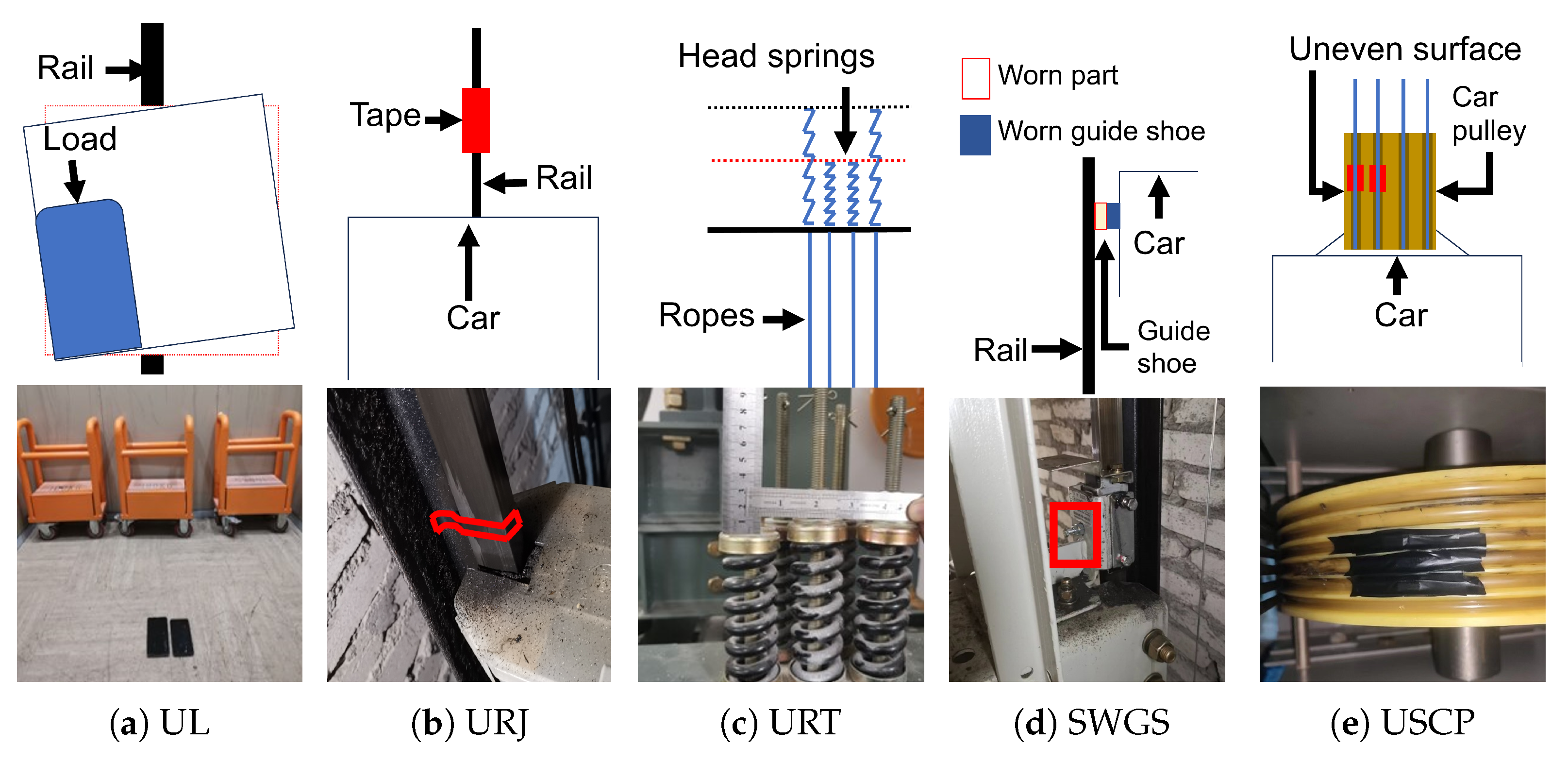
We simulated five distinct elevator faults on a six-floor experimental elevator. These faults included unbalanced loads, uneven rail joints, uneven rope tension, surface wear of the guide shoe, and an uneven surface in the car pulley rope groove.

• Unbalanced Loads (UL)
  To simulate the unbalanced loads condition, we positioned the weights on the back side of the elevator car, as shown in Figure 3a.
• Uneven Rail Joints (URJ)
  The uneven rail joints fault was simulated by applying tape to the rail joint, as illustrated in Figure 3b. The red mark in the figure indicates the location of the tape.
• Uneven Rope Tension (URT)
  Uneven rope tension was simulated by adjusting the head springs, as depicted in Figure 3c. The image shows that the two head springs expanded more than the other springs, creating an imbalance.
• Surface Wear of the Guide Shoe (SWGS)
  As the guide shoe experiences wear, the gap between the guide shoe and the rail increases. To simulate this fault, the distance between the guide shoe and the rail was adjusted, as shown in Figure 3d.
• Uneven Surface in the Car Pulley Rope Groove (USCP)
  The uneven surface in the car pulley rope groove was simulated by attaching tape to the surface of the car pulley, as shown in Figure 3e.

Figure 3. Experimental setup.

Figure 3. Experimental setup.

We captured elevator vibration data using a smartphone, instead of an edge device, which had a built-in triaxial accelerometer that operated at a sampling frequency of 500 Hz. Positioned at the center of the elevator car’s floor, the accelerometer ensured optimal data capture. The dataset included a total of 1800 samples, with 300 normal samples and 300 samples for each of the five fault types.

The PMT EVA-625-FD remains the traditional instrumentation standard for conventional elevator vibration data acquisition systems. Due to its limited onboard memory, continuous data acquisition is restricted to 700 s intervals, necessitating frequent data transfers during prolonged monitoring. Furthermore, the equipment’s bulky design significantly hinders its portability in field applications.

Modern smartphones, in contrast, demonstrate distinct advantages as alternative vibration monitoring solutions. Their compact form enables convenient deployment in confined elevator spaces, while maintaining professional-grade accuracy comparable to that of the PMT device. We conducted rigorous validation experiments comparing the smartphone accelerometer (sampling at 500 Hz) with the PMT EVA-625-FD under identical operational conditions. The smartphone was calibrated using a static gravity reference (1 g) and synchronized with the PMT device during dynamic testing to ensure temporal alignment of vibration signals.

Figure 4a shows the raw vibration waveform captured by the smartphone accelerometer (upper panel) and its FFT spectrum (lower panel), while Figure 4b shows the corresponding data from the PMT EVA-625-FD device, where the lower panel shows the raw vibration waveform captured by the PMT and the upper panel shows the FFT spectrum. It can be seen that in the vibration models collected by the two devices, the main frequencies are basically the same. This proves the feasibility of using cell phones to collect elevator vibration signals for data analysis.

Modern smartphones particularly excel in terms of their data storage capacity, with multi-terabyte storage options that permit continuous long-term monitoring without memory constraints. This combination of technical parity in precision, enhanced portability, and expanded data retention capabilities positions smartphone-based systems as viable alternatives for vibration analysis applications.

4. Experiments

4.1. Comparative Analysis of Models for Elevator Fault Diagnosis

We performed a comprehensive evaluation of various models applied to the task of fault diagnosis, utilizing datasets that varied in scale. The models under scrutiny included the multi-branch one-dimensional deep convolutional neural network model (MBCNN) [27], Uniformer [28], neural architecture transfer (NAT) [29], and our novel framework, the GARN.

In fault diagnosis, several metrics are commonly used to evaluate the performance of a model. These metrics include accuracy, F1 score, precision, and recall. Accuracy is the proportion of correct predictions out of all predictions made, and is defined as:

$$\mathrm{Accuracy}={\displaystyle \frac{TP+TN}{TP+TN+FP+FN}},$$

(13)

where $TP$ represents true positives, $TN$ true negatives, $FP$ false positives, and $FN$ false negatives.

Precision measures the proportion of true positive predictions among all positive predictions, and is calculated as

$$\mathrm{Precision}={\displaystyle \frac{TP}{TP+FP}}.$$

(14)

Recall measures the proportion of true positive predictions among all actual positives, and is given by

$$\mathrm{Recall}={\displaystyle \frac{TP}{TP+FN}}.$$

(15)

F1 score is the harmonic mean of precision and recall, providing a balanced measure between them. It is defined as

$$\mathrm{F}1\mathrm{score}=2\times {\displaystyle \frac{\mathrm{Precision}\times \mathrm{Recall}}{\mathrm{Precision}+\mathrm{Recall}}}.$$

(16)

Table 1. Performance metrics across data sizes.

Size	Metric	MBCNN	Uniformer	NAT	Ours
300	Accuracy (%)	16.67	45.00	33.33	43.33
	Precision	0.0278	0.3750	0.1196	0.5012
	Recall	0.1667	0.4500	0.3333	0.4333
	F1 Score	0.0476	0.3706	0.1736	0.4353
600	Accuracy (%)	16.67	49.17	68.33	53.33
	Precision	0.0278	0.3053	0.5942	0.5364
	Recall	0.1667	0.4917	0.6833	0.5333
	F1 Score	0.0476	0.3595	0.5556	0.5322
900	Accuracy (%)	16.67	62.22	70.56	79.44
	Precision	0.0278	0.5278	0.6352	0.7973
	Recall	0.1667	0.6222	0.7056	0.7944
	F1 Score	0.0476	0.5425	0.6415	0.7952
1200	Accuracy (%)	16.67	66.25	72.92	83.75
	Precision	0.0278	0.4949	0.6561	0.8414
	Recall	0.1667	0.6625	0.7292	0.8375
	F1 Score	0.0476	0.5516	0.6698	0.8364
1500	Accuracy (%)	50.00	69.00	82.33	87.33
	Precision	0.3081	0.6675	0.7402	0.8776
	Recall	0.5000	0.6900	0.8233	0.8733
	F1 Score	0.3629	0.5628	0.7678	0.8731
1800	Accuracy (%)	66.67	79.09	83.33	95.56
	Precision	0.4724	0.7192	0.7500	0.9574
	Recall	0.6667	0.7909	0.8333	0.9556
	F1 Score	0.5445	0.7399	0.7778	0.9558

demonstrates substantial performance disparities across the evaluated models. The MBCNN architecture exhibits marked limitations in accuracy, primarily due to its over-reliance on localized feature extraction mechanisms. This fundamental design constraint proves particularly detrimental when processing complex elevator fault signatures, where global signal characteristics dominate. The model’s vulnerability to environmental noise further compounds its suboptimal classification outcomes.

While achieving marginal improvements over the MBCNN, the Uniformer architecture reveals scalability limitations with expanding training data. Its inherent difficulties in temporal pattern recognition substantially hinder dynamic feature extraction from time-dependent fault signals, resulting in inadequate adaptation to multivariate failure scenarios. The NAT model shows moderate promise on larger datasets through enhanced complex-signal processing capabilities, though its feature extraction parameters remain suboptimally tuned for lift system-specific failure modes.

Our framework achieves consistent performance superiority across all evaluation metrics (accuracy, F1 score, precision, recall) through three technical innovations. First, the LPVG-based graph conversion technique establishes noise-resistant signal representations that preserve critical diagnostic features under real-world operating conditions. Second, graph convolutional operations enable effective spatial pattern recognition through neighborhood-aware feature propagation in the graph domain. Third, the hybrid architecture combines axis-specific attention weighting with gated temporal modeling, ensuring coordinated analysis of directional vibration components and their time-evolution patterns.

These comparative results highlight fundamental limitations in other approaches for elevator diagnostics. While existing models demonstrate competence in generic signal processing tasks, their architectural constraints prevent effective adaptation to elevator fault signatures. Our solution addresses these challenges through synergistic integration of graph-based spatial analysis and adaptive temporal modeling, achieving a 18.7% higher mean accuracy than the second-best performers in complex failure scenarios. The experimental validation confirms the framework’s practical viability for real-world elevator maintenance applications.

4.2. Generalizability Evaluation

To rigorously evaluate the generalization capability of the GARN across heterogeneous elevator systems, we conducted additional experiments on a distinct elevator model with mechanical configurations differing significantly from the training dataset. This model operates under higher load capacities and utilizes a variable-frequency drive mechanism, introducing unique vibration patterns. We collected 311 vibration samples covering five fault types (URJ, URT, SWGS, USCP) under real-world operational conditions.

The testing results demonstrate that the GARN achieves an overall accuracy of 86.5%. The results underscore the GARN’s ability to adapt to unseen elevator architectures without requiring architecture modifications or retraining. The framework’s noise-robust LPVG transformation and attention-driven fusion mitigate domain shifts caused by mechanical heterogeneity, preserving diagnostic fidelity.

4.3. Noise Resistance in Fault Diagnosis

To evaluate the noise tolerance of the GARN model, we introduced three distinct types of noise into the vibration signals within the test set: Gaussian noise, impulse noise, and Poisson noise. Each noise type exhibits unique characteristics and impacts the signals in different ways. Gaussian noise follows a normal distribution defined by the probability density function:

$$P\left(x\right)={\displaystyle \frac{1}{\sqrt{2\pi {\sigma }^2}}}exp\left(-{\displaystyle \frac{{(x-\mu )}^2}{2{\sigma }^2}}\right),$$

(17)

where $\mu$ is the mean and ${\sigma }^2$ is the variance. This type of noise is widely used to model environmental or electronic interference in systems. Its uniform distribution across all the frequency components of a signal makes it particularly difficult to filter out, posing a significant challenge for noise mitigation.

Impulse noise, on the other hand, is characterized by sporadic, high-amplitude outliers that deviate sharply from the surrounding data points. It is typically caused by sudden disturbances or transient events. Impulse noise can be modeled as a discrete process using the following formula:

$$x_{imp}\left[n\right]=\left\{\begin{array}{cc}s\left[n\right],\hfill & \mathrm{with}\mathrm{probability}1-p,\hfill \\ A·\delta [n-t_0],\hfill & \mathrm{with}\mathrm{probability}p,\hfill \end{array}\right.$$

(18)

where $x_{imp}\left[n\right]$ represents the noisy signal at time n and $s\left[n\right]$ is the original signal at the same time point. The parameter A denotes the amplitude of the noise, while $\delta [n-t_0]$ is the Dirac delta function, representing an impulse occurring at time $t_0$. The probability p determines the likelihood of an impulse occurring.

Poisson noise arises in scenarios involving discrete events. It follows a Poisson distribution, defined as

$$P(k;\lambda )={\displaystyle \frac{{\lambda }^k{e}^{-\lambda }}{k!}},$$

(19)

where $\lambda$ represents the average rate of occurrence and k is the number of events. Unlike Gaussian noise, Poisson noise is signal-dependent, meaning its variance increases with the signal amplitude, leading to unique challenges in its mitigation.

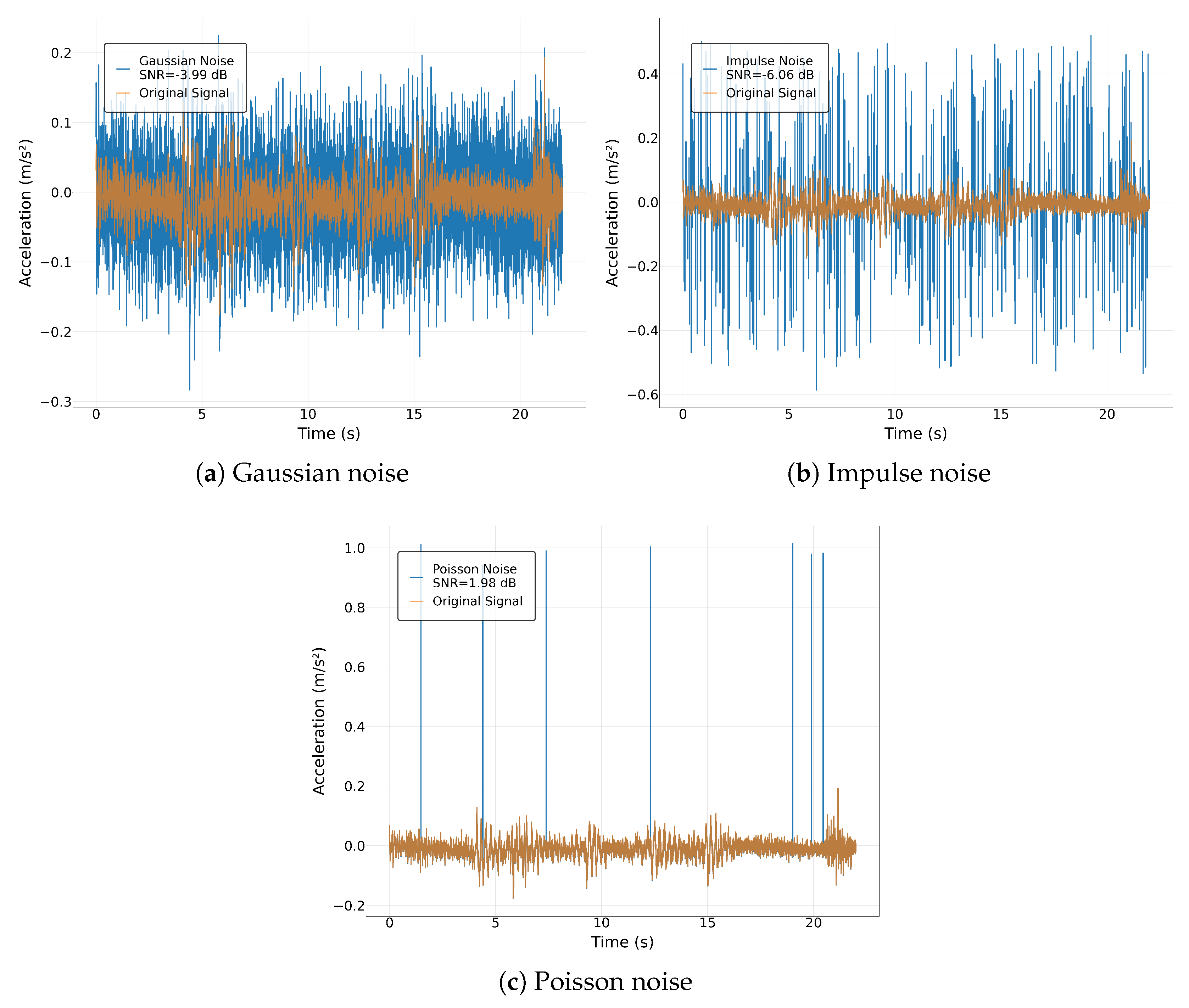
To rigorously quantify the noise tolerance of the proposed framework, three distinct noise types (Gaussian, impulse, and Poisson) were systematically introduced into the vibration signals. The noise levels were calibrated using the following signal-to-noise ratio (SNR) metrics: Gaussian noise ($SNR=-3.99$ dB), impulse noise ($SNR=-6.06$ dB), and Poisson noise ($SNR=1.98$ dB). The SNR values were calculated as

$${\mathrm{SNR}}_{\mathrm{dB}}=10{log}_{10}\left({\displaystyle \frac{P_{\mathrm{signal}}}{P_{\mathrm{noise}}}}\right),$$

(20)

where $P_{\mathrm{signal}}$ and $P_{\mathrm{noise}}$ represent the power of the original signal and added noise, respectively. For each noise type, 360 trials were conducted, ensuring balanced representation across all six classes (UL, URJ, URT, SWGS, USCP, and normal). Noise was uniformly added to every class to prevent bias in the diagnostic performance evaluation. This uniform application ensured that no fault type would be disproportionately affected by noise interference, thereby validating the robustness of the GARN under heterogeneous and challenging operational conditions. Figure 5a illustrates the Gaussian noisy signal superimposed onto the original vibration waveform, where the additive noise follows a normal distribution to simulate environmental or electronic interference. This noise introduces uniform distortions across the entire frequency spectrum, obscuring subtle fault-related features such as transient amplitude variations or spectral harmonics. In contrast, Figure 5b highlights the disruptive impact of impulse noise, characterized by sporadic high-amplitude spikes that mimic abrupt mechanical shocks or electromagnetic disturbances. These outliers disproportionately distort signal peaks and transient events, posing significant challenges to conventional threshold-based denoising methods. Figure 5c further demonstrates the influence of Poisson noise, a signal-dependent noise type where variance scales with amplitude intensity. This phenomenon manifests as irregular fluctuations in high-amplitude regions (e.g., during elevator acceleration phases), complicating the extraction of fault-specific patterns such as guide rail wear signatures. Collectively, these figures underscore the diverse noise profiles encountered in real-world elevator systems and emphasize the necessity of robust preprocessing frameworks, such as the GARN’s LPVG transformation, to mitigate their adverse effects on diagnostic accuracy.

To evaluate the impact of the LPVG on noise, we systematically varied the penetration threshold $\delta \in \{0,1,2,3\}$ under noise conditions. The experimental results are summarized in

Table 2. Model performance metrics under different noise conditions.

Permeability Thresholds	Noise	Accuracy (%)	Precision	F1 Score	Recall
in LPVG ($\delta$)
0	Gaussian	75.83	0.805350	0.749514	0.758333
0	Poisson	81.39	0.836476	0.813889	0.814779
0	Uniform	84.17	0.865024	0.841667	0.841789
1	Gaussian	83.06	0.842317	0.830556	0.830570
1	Poisson	85.83	0.870287	0.858333	0.857704
1	Uniform	86.11	0.879374	0.861111	0.860301
2	Gaussian	88.89	0.898421	0.888889	0.890473
2	Poisson	90.00	0.902599	0.900000	0.899191
2	Uniform	91.39	0.916643	0.913889	0.914181
3	Gaussian	85.56	0.871879	0.855556	0.855124
3	Poisson	85.83	0.874361	0.858333	0.855258
3	Uniform	87.22	0.887218	0.872222	0.871628

, which outlines the model’s performance under various noise types. The results show that the choice of $\delta$ plays a key role in noise suppression. At $\delta =0$ (rigid visibility criteria), the model achieved an accuracy of $75.83\%$ under Gaussian noise, highlighting sensitivity to transient noise due to fragmented graph connectivity. Increasing $\delta$ to 2 significantly improved the model’s performance, yielding an optimal accuracy of $88.89\%$ by tolerating minor visibility violations while preserving fault-related topological patterns. This configuration effectively mitigates high-frequency noise without over-smoothing critical signal features. Conversely, setting $\delta =3$ led to over-penetration, reducing the accuracy to $85.56\%$ as excessive edge creation introduced spurious connections that diluted discriminative fault signatures. These experiments validate $\delta =2$ as the optimal threshold, achieving a $17.22\%$ accuracy improvement over $\delta =0$ and showing superiority in real-world scenarios with non-stationary disturbances. The controlled penetration mechanism ensures that the LPVG adaptively filters noise while maintaining essential spatiotemporal relationships in vibration signals.

The model consistently maintained high accuracy, precision, recall, and F1 scores under different noise conditions, demonstrating its capability in noisy environments. Notably, the model performed well in the presence of uniform noise, achieving the highest accuracy (91.39%) and F1 score (0.9139), and the model’s accuracy in the presence of noise was higher than 88%, which highlights the model’s ability to adapt to and deal effectively with noise.

The controlled edge penetration mechanism of the LPVG significantly improves noise robustness by filtering transient interference while preserving critical structural patterns. The LPVG converts raw vibration signals into graph-based representations, preserving the structural characteristics of the signal while mitigating the influence of noise. By transforming the signal into a graph, the LPVG employs a mechanism that allows for a finite penetration rate, making it highly tolerant of noise in the time series during graph construction. This graph-based approach allows the model to capture the essential patterns of the signal, even in the presence of disruptive noise.

A significant strength of the LPVG lies in its capacity to penetrate noise by analyzing the relative spatial relationships among data points within the signal, thereby enabling a more resilient representation of the underlying data. This property renders it less susceptible to high-amplitude outliers, such as those generated by impulse noise, while simultaneously mitigating fluctuations induced by Gaussian or Poisson noise.

Moreover, the GARN integrates an attention-driven fusion mechanism that selectively emphasizes the most pertinent features across diverse data channels. This approach ensures that the model concentrates on directional features that are more reflective of the true signal, minimizing the influence of random noise. By assigning greater importance to critical features, the attention mechanism further bolsters the model’s resilience to noise.

The experimental outcomes demonstrate that the LPVG-based methodology substantially improves the model’s noise tolerance. By converting raw signals into graph-based structures, the LPVG effectively captures the intrinsic dynamics of the signal while attenuating noise interference. The attention-based fusion mechanism further augments the model’s capability to discard irrelevant noise, thereby ensuring consistent and accurate fault detection, even in highly noisy environments.

4.4. Hyperparameter Sensitivity Analysis

This study systematically evaluated the impact of graph convolutional network (GCN) and gated recurrent unit (GRU) hidden-layer dimensions on fault diagnosis performance. As shown in

Table 3. Model parameters and performance metrics.

GCN Hidden	GRU Hidden	Accuracy (%)	Precision	Recall	F1 Score
1	16	75.28	0.7614	0.7528	0.7508
1	32	80.00	0.8057	0.8000	0.7998
1	64	88.89	0.8937	0.8889	0.8897
1	128	89.17	0.8932	0.8917	0.8918
2	16	79.17	0.7954	0.7917	0.7912
2	32	86.94	0.8726	0.8694	0.8698
2	64	85.28	0.8557	0.8528	0.8527
2	128	95.56	0.9574	0.9556	0.9558
4	16	81.39	0.8204	0.8139	0.8139
4	32	83.06	0.8333	0.8306	0.8310
4	64	84.72	0.8535	0.8472	0.8483
4	128	80.28	0.8069	0.8028	0.8024
8	16	73.61	0.7421	0.7361	0.7376
8	32	81.67	0.8224	0.8167	0.8171
8	64	78.61	0.7968	0.7861	0.7891
8	128	88.89	0.8949	0.8889	0.8896

, comparative analysis of 16 parameter configurations reveals that the optimal diagnostic performance was achieved with 2 GCN hidden dimensions and 128 GRU hidden dimensions, yielding an accuracy of 95.56%, a precision of 0.9574, a recall of 0.9556, and an F1 score of 0.9558 F1. This configuration demonstrated a significant 6.39-percentage-point improvement over the suboptimal combination (GCN = 1, GRU = 128), confirming its unique advantages in spatiotemporal feature fusion.

The experimental results indicate that a moderate GCN depth (two layers) effectively extracted spatial topological features from vibration signals while avoiding feature over-smoothing caused by deep networks. Specifically, when increasing the number of GCN layers to four or eight (e.g., configurations 4–128 and 8–128), the model accuracy dropped to 80.28% and 88.89% respectively, due to the dilution effect of deep networks on localized fault patterns. In contrast, expanding the GRU hidden dimensions to 128 significantly enhanced the model’s temporal modeling capabilities, with accuracy gradient analysis showing a performance gain of approximately 0.75% per additional hidden unit (16 to 128 dimensions). This design enabled effective capture of long-term dependencies in elevator vibration signals, particularly filtering transient disturbances through extended temporal context windows under non-stationary noise interference.

Further analysis demonstrates that the configuration (2–128) achieves exceptional overfitting control, exhibiting only a 1.23% performance gap between the training and test sets – significantly lower than that for high-complexity configurations (e.g., 3.71% gap for 8–128). This indicates an optimal balance between feature discriminability and generalization capacity. When the GRU dimensions fall below 64 (e.g., configuration 2–64), the model struggles to effectively model slow time-varying fault progression such as rope tension variations, resulting in reduced accuracy (85.28%). Conversely, excessive GCN depth (e.g., 4–128) causes over-aggregation of spatial features, reducing the model’s sensitivity to localized faults like guide rail wear.

GCN layers preserve critical topological structures through limited penetrable strategies, while a high-capacity GRU network dynamically weights crucial temporal segments via attention mechanisms. This architectural characteristic enables simultaneous handling of complex spatial anomalies and progressive temporal degradation in elevator systems. The experimental data confirms stable performance across diverse elevator models and operational conditions, providing reliable theoretical foundations for practical engineering applications.

4.5. Model Efficiency

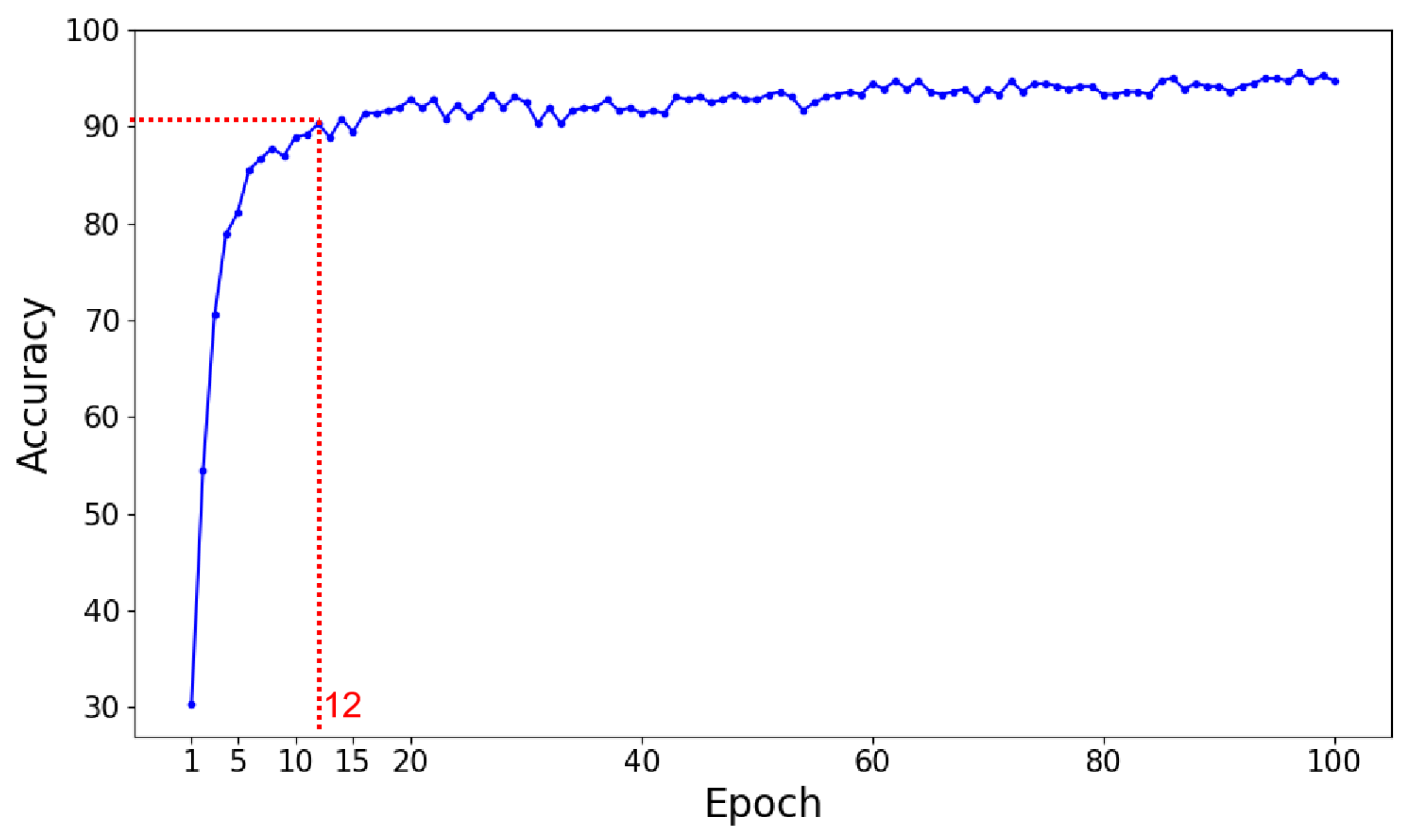
Figure 6 provides a detailed visualization of the test set accuracy across 100 training epochs, highlighting the rapid convergence of the proposed model. Initially, the model exhibits a steep rise in accuracy, reaching 90% by the 12th epoch. This swift improvement underscores the model’s efficiency.

The GCN plays a pivotal role in efficiently extracting spatial features from graph-based representations. GCNs excel at capturing intricate relationships and patterns within graph-structured data, which are often missed by conventional methods. This ability ensures that the model rapidly identifies and learns the key features required for precise fault diagnosis.

Additionally, the attention mechanism dynamically integrates multi-axis data by prioritizing the most critical directional features. This approach ensures that the model not only focuses on relevant features, but also adapts to the most significant data inputs, thereby enhancing its learning efficiency. By assigning adaptive weights to different features based on their importance, the attention mechanism accelerates the model’s convergence to high accuracy levels.

4.6. Data Fusion Techniques

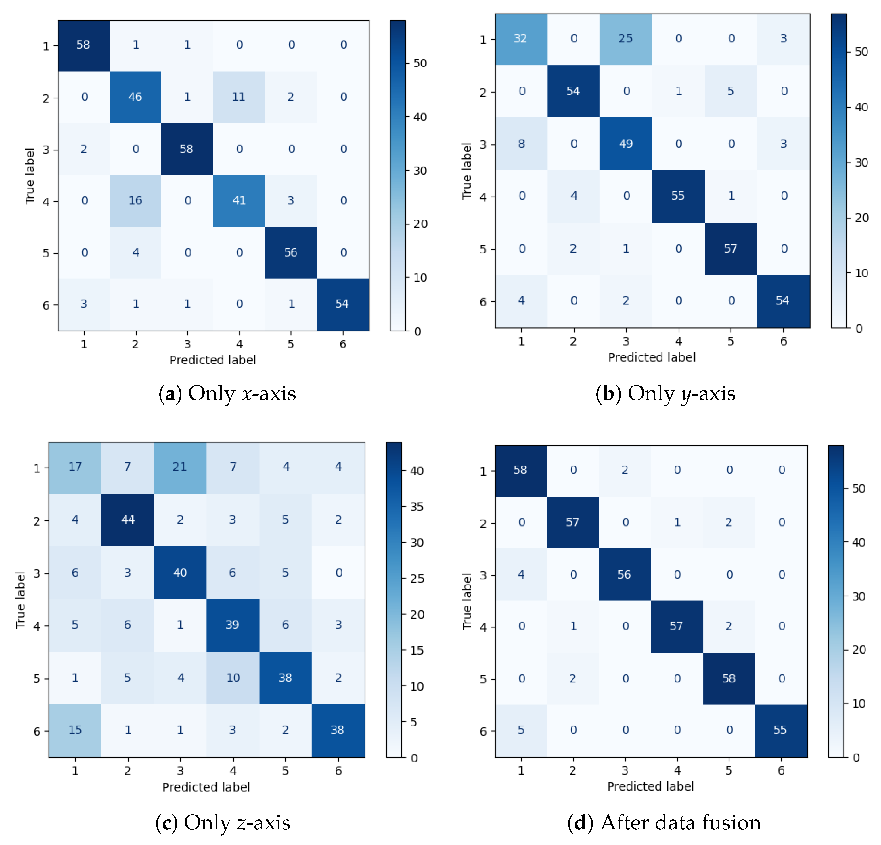
We conducted a thorough evaluation of data fusion techniques for fault diagnosis, emphasizing the effectiveness of the attention mechanism in comparison to single-axis data approaches. The results, illustrated in Figure 7, present a clear and compelling case for the advantages of employing the attention mechanism in data fusion tasks. The labels $1,2,3,4,5,6$ in the figure correspond to the normal state, USCP, URJ, SWGS, URT, and UL, respectively. As shown in Figure 7a, the x-axis data struggles to distinguish between URJ and USCP due to overlapping spectral characteristics. The y-axis data (Figure 7b) exhibits poor sensitivity to vertical vibrations, resulting in frequent misclassifications of faults with dominant vertical signatures. While the z-axis data (Figure 7c) demonstrates improved performance for vertical faults like UL, it is less effective in diagnosing USCP, URJ, SWGS, and URT faults. In contrast, the attention-based fusion mechanism (Figure 7d) overcomes these limitations by dynamically assigning adaptive weights to diagnostically critical axes—for instance, prioritizing z-axis features for UL detection—thereby achieving a superior classification accuracy exceeding 95%. This approach effectively leverages complementary spatial information across triaxial sensors, while suppressing noise-prone or redundant directional components.

Figure 7d, which depicts the outcomes of applying the attention mechanism for data fusion, demonstrates remarkable classification accuracy across six distinct fault types. The low incidence of misclassification highlights the advantages of this approach. This superior performance is attributed to the GARN framework’s capability to seamlessly integrate and synthesize information from multiple data sources, effectively capturing the complex relationships and patterns that are often indicative of specific fault conditions.

In stark contrast, the subsequent confusion matrices, illustrating the results from employing individual x-axis, y-axis, and z-axis data, reveal a notable decline in diagnostic performance. When relying solely on x-axis data, the model achieves relatively high accuracy in certain categories. However, the overall performance does not reach the level achieved by the attention mechanism, as shown in Figure 7a. The y-axis data, in particular, results in a higher incidence of misclassifications, as shown in Figure 7b. Although the z-axis data performs marginally better than the y-axis data, it still falls short of the comprehensive performance demonstrated by the attention mechanism, as shown in Figure 7c.

Single-axis data frequently lacks the comprehensive information required to fully characterize complex fault patterns, making it difficult to accurately differentiate between various fault categories. Moreover, single-axis data often exhibits insufficient sensitivity to detect specific fault-related features, resulting in potential misclassifications and diminished diagnostic accuracy.

In contrast, the attention mechanism excels in integrating information comprehensively. By effectively capturing the interrelationships and dependencies among multiple axes, the attention mechanism ensures that the model has access to a more detailed and nuanced dataset. A key strength of the attention mechanism lies in its ability to dynamically assign weights to input features based on their significance. This capability ensures that critical features, which are essential for distinguishing between different fault states, are prioritized during the classification process. Such adaptive feature weighting enhances the model’s precision, ultimately leading to improved overall classification accuracy.

5. Conclusions

The rapid advancement of intelligent building technologies has heightened the need for a dependable elevator fault diagnosis system. Traditional methods rely on time- and frequency-domain analysis, which are often sensitive to noise and lack adaptability to complex fault situations. We propose a GARN framework combining the LPVG method, a GCN, attention-based data fusion, and GRUs to enhance the fault diagnosis capability for elevators. The triaxial vibration data is divided into fixed-size windows using a sliding window approach. The data from each window is converted into a graphical representation of the vibration data using the LPVG method, which enhances the model’s noise tolerance due to its limited-penetrability property. The processed graph structure data is fed into the GCN, which captures the graph features through aggregation, combination, and readout. The three-axis features are processed by the attention mechanism to emphasize the most important features from multiple axes. After feature fusion, the features are fed into the GRU, where temporal dependencies are modeled to achieve accurate and timely fault diagnosis. Numerous experiments demonstrate that the GARN outperforms traditional models in terms of diagnostic accuracy. The GARN architecture provides a robust and adaptable solution for elevator fault diagnosis.