A Segmented Adaptive PID Temperature Control Method Suitable for Industrial Dispensing System

Abstract

Industrial dispensing systems consist of many components, and the temperature characteristics of these components vary significantly. To address this, a segmented adaptive PID temperature control method is proposed in this paper. This method integrates a segmented temperature control algorithm with a variable control coefficient algorithm based on output power, which not only ensures minimal overshoot in the system but also enhances its disturbance rejection capability. Experimental results demonstrate that, under identical conditions, compared with the traditional PID method, the proposed method reduces overshoot by 2–4 °C and decreases the amplitude of temperature fluctuations after disturbance by approximately 0.2 °C.

1. Introduction

Precision temperature control is a critical technology in industrial glue dispensing systems. To ensure stable product quality from the dispensing applicator, various components, such as the press plate, quantitative filling machine valves, heating module, glue gun copper sleeve, and glue gun valve block, need to be stabilized at specific temperatures. It is also essential to minimize temperature fluctuations and maximize disturbance rejection capability.

In the traditional PID algorithm, tuning and setting the proportional coefficient, integral coefficient, and derivative coefficient for a specific controlled object are necessary [1,2]. The traditional approach involves determining the PID coefficients based on specific tuning rules after deriving the mathematical model of the object. Examples of such methods include the Ziegler–Nichols method [3,4], the pole placement method [5], the M-constrained Integral Gain Optimization tuning method [6], the Kappa-Tau method [7], and the Internal Model Control tuning method [8,9].

However, in industrial dispensing systems, many controlled processes exhibit distinct characteristics due to their complex mechanisms, including nonlinearity, time-varying uncertainty, and time lag. When operating conditions change, the system’s model parameters will shift, and in some cases, the controller structure may also need adjustment [10]. Consequently, the previously tuned coefficients can no longer ensure the control system’s performance, necessitating the timely adjustment of these coefficients [11].

Consequently, traditional PID controllers demonstrate significant limitations in industrial dispensing systems, primarily manifesting as follows:

• Challenges in achieving optimal parameter tuning
• Excessive temperature overshoot
• Suboptimal control precision
• Prolonged convergence times

To enhance the control performance of temperature control systems with time-delay characteristics, studies [12,13,14,15] have proposed a control strategy where a fuzzy controller adjusts PID parameters online. References [16,17,18] present the concept of optimizing the proportional factor in the fuzzy controller using an improved particle swarm optimization algorithm, thereby addressing the issue of defuzzification control overly relying on expert experience. Studies [19,20,21,22,23] have proposed leveraging the neural network’s self-learning ability to automatically tune the parameters of traditional PID algorithms. However, both of these methods exhibit high computational complexity, imposing strict requirements on the controller’s computational performance and implicitly increasing the production costs for equipment manufacturers.

In response to these limitations of traditional temperature control approaches, this paper proposes an adaptive PID temperature control method.

The subsequent sections of this paper are organized as follows. In Section 2, the preliminary research begins with the system architecture and heat transfer model, expounds on the composition of the multi-channel heating system, and establishes the transfer function through experiments, providing a theoretical foundation for the subsequent design of the control algorithm. In Section 3, a segmented temperature control algorithm is proposed and further divided into four stages. In Section 4, an adaptive PID tuning method based on output power is proposed to enhance the system’s disturbance rejection capability. In Section 5, experiments are conducted to compare and validate the algorithm’s advantages in terms of overshoot and disturbance rejection performance. Section 6 finally summarizes the method’s applicability in industrial scenarios.

2. Preliminary Studies

This section primarily introduces the temperature control requirements and transfer function model of the industrial glue dispensing heating system, laying the foundation for the subsequent temperature control algorithm.

2.1. The Structure of Industrial Dispensing Temperature Control System

As shown in Figure 1a,b, the industrial glue dispensing heating system primarily consists of a multi-channel thyristor heater (TH), an industrial glue dispenser, a multi-channel temperature sampling device, and an embedded temperature controller. The TH, positive temperature coefficient (PTC) ceramic heating plates, thermocouple, and the device under test (DUT) are all located at the production site.

During system operation, the TH provides heat to the DUT via the ceramic heating plates. The temperature sensors (one sensor per channel) continuously monitor the temperature and feed this information back to the controller. The embedded temperature controller employs intelligent algorithms to precisely regulate the TH’s output power, ensuring that each part of the DUT maintains its set temperature.

The industrial glue dispensing system features five independent temperature control channels (shown in Figure 1a), each with different target temperatures set according to the production process. This design allows for progressive heating of the glue within the DUT, starting from the pressure plate, passing through multiple components, and finally reaching the glue gun valve, where the glue temperature precisely meets the required process specifications.

Five independent heating channels are employed because the glue flow in the dispensing system is intermittent, and the long transmission path renders a single channel incapable of achieving precise temperature control throughout the system. Multiple independent temperature control channels enable each component to gradually attain and sustain the desired temperature, thereby ensuring that the glue temperature at the glue gun valve is maintained within ±0.3 °C.

Correspondingly, in the embedded controller of the industrial dispensing system, the temperature control program is divided into five channels, with each channel executing an independent PID algorithm to control its corresponding channel at the respective target temperature.

Considering the potential interference among channels during glue flow, this paper later discusses the disturbance rejection measures and performance of the proposed algorithm. Specifically, Section 4 delves into how the system manages disturbances caused by intermittent glue flow, ensuring robust temperature control even under dynamic conditions.

2.2. Transmission Model of the Heating System

Here, taking the heating module components in the system as an example, the transfer function is determined using the following experimental method.

The heat transfer process of the dispensing system exhibits remarkable thermal inertia and pure lag characteristics:

Thermal Inertia: Temperature changes in heating components (e.g., nozzles or adhesive containers) occur via heat conduction or convection, with their response speed limited by the thermal conductivity of materials and component volume.

Pure Lag: The response delay of temperature sensors, signal transmission delay within the heating circuit, and thermal diffusion delay caused by adhesive flow in pipelines all contribute to pure lag.

Therefore, in the experiment, the temperature control system model of the heating module is approximated as a First-Order Plus Dead Time (FOPDT) model. The time constant T in the FOPDT model quantifies the time required for the system to reach steady-state temperature, directly reflecting the influence of thermal inertia. The lag time $\tau$ in the model reflects the time-delay characteristics of the system. Therefore, the transfer function of the model is expressed by the following formula:

$$G(s)={\displaystyle \frac{K}{Ts+1}}\times e^{-\tau s}$$

(1)

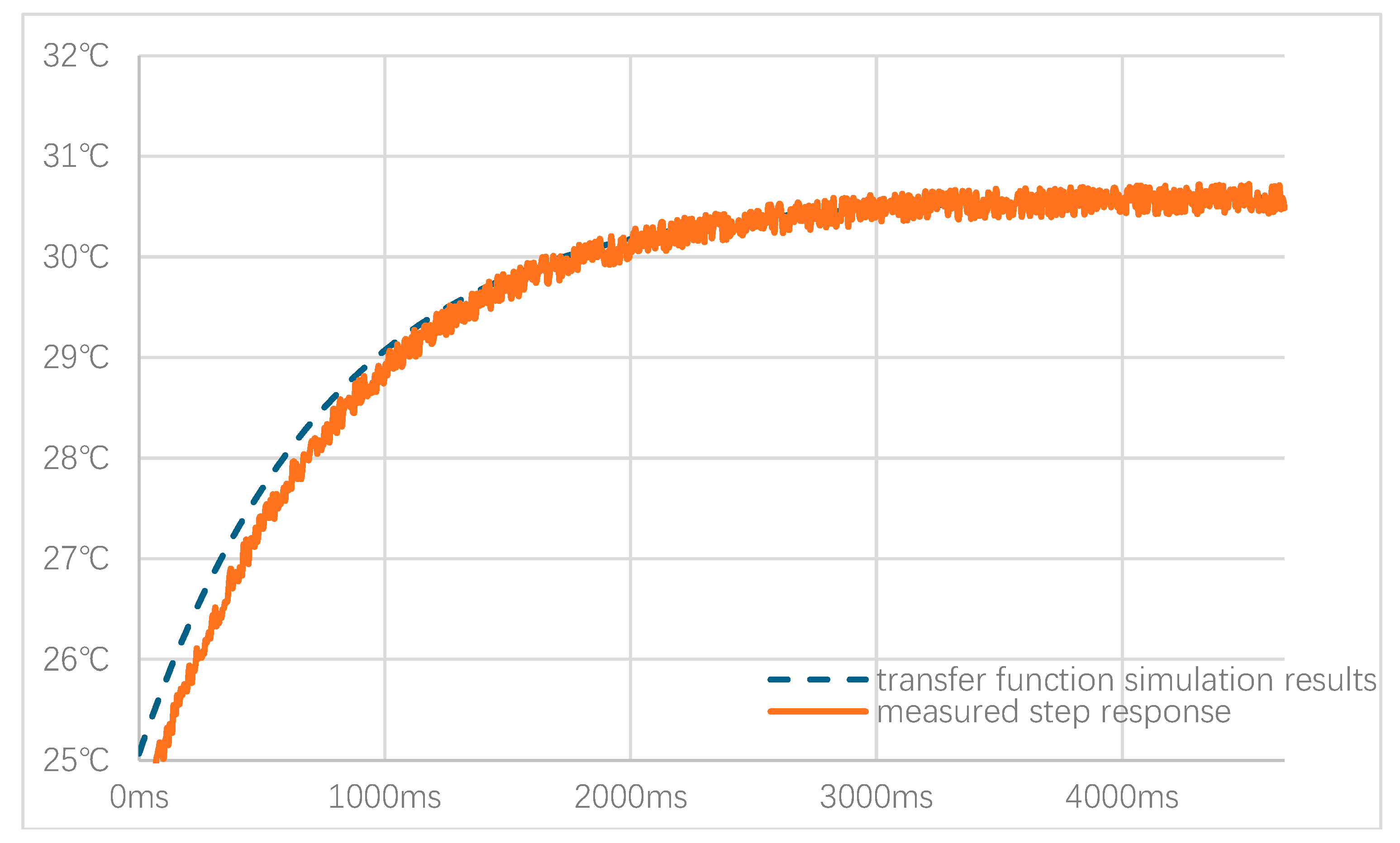
The step response method is commonly used to identify the transfer function of a control system. In the glue dispensing temperature control system, when a fixed-amplitude voltage is applied, the system’s transfer function can be derived from the temperature response curve. Figure 2 illustrates the step response temperature curve of the DUT’s heating module channel in the experiment. The solid line represents the measured temperature from the step response, while the dashed line shows the model simulation results using parameters obtained from data fitting (the parameter estimation method is described in Equations (2)–(7)). In the step response experiment, the heater is a PTC ceramic heating element; the control voltage is fixed at 5 volts starting at time 0, and the initial temperature is set as the coordinate system origin.

According to the FOPDT model, the step response of the temperature control system is described by Equation (2) in the Laplace domain.

$$F(s)=G(s)\times U(s)$$

(2)

Here, $F(s)$ represents the system’s response in the Laplace domain, and $U(s)$ represents the Laplace transform of the control signal. The transient process of the control system in the time domain is described by the following formula:

$$F(s)={\displaystyle \frac{K}{Ts+1}}{e}^{-\tau s}\times {\displaystyle \frac{A}{s}}$$

(3)

$$f(t)=L^{-1}[F(s)]=K\times A(1-e^{-(t-\tau )/T})u(t-\tau )$$

(4)

Here, $A$ is the amplitude of the step input, $u(t-T)$ is the unit step function, and $L^{-1}$ denotes the inverse Laplace transform. It can be observed from the above formula that when the steady-state condition $t\to \infty$ is satisfied, the step response tends to $K·A$.

The value of $K$ in the transfer function can be calculated according to the following formula:

$$K={\displaystyle \frac{f(\infty )-f(0)}{u(\infty )-f(0)}}$$

(5)

$$\left\{\begin{array}{c}{\displaystyle \frac{f(\infty )-f(t_1)}{f(\infty )}}=e^{\left({\displaystyle \frac{\tau }{T}}-{\displaystyle \frac{t_1}{T}}\right)}\\ {\displaystyle \frac{f(\infty )-f(t_2)}{f(\infty )}}=e^{\left({\displaystyle \frac{\tau }{T}}-{\displaystyle \frac{t_2}{T}}\right)}\end{array}\right.$$

(6)

The ambient temperature is 25.5 °C, which is taken as the reference point for the temperature-time curve. The initial temperature must be subtracted from the step response curve. According to the principle mentioned above, the calculation of the parameter $K$ is outlined in Formula (5).

The calculation of $T$ and $\tau$ requires taking two known points in the system response, as shown in Formula (6). From Figure 2, the measured temperatures at $t_1=0 \mathrm{ms}$ and $t_2=4600 \mathrm{ms}$ can be obtained. By substituting the temperature values at these two moments into Equation (6), the values of the three parameters can be solved as $K=15.5$, $T=155.5$, $\tau =16$. Therefore, the transfer function can be expressed by the following formula:

$$G(s)={\displaystyle \frac{15.5}{155.5s+1}}{e}^{-16s}$$

(7)

Using the same method, the heat transfer functions of other channels can be measured. The solution process is omitted here.

3. Proposed Method: Segmented Temperature Control Algorithm

References [24,25,26] suggest that the PID algorithm can be integrated with the time-optimal algorithm. When the temperature error exceeds the threshold, the time-optimal algorithm applies maximum power heating to raise the heated body’s temperature in the shortest time. When the temperature error falls below the threshold, the PID algorithm alone regulates the output power to stabilize its temperature. This approach reduces system overshoot, but due to the varying thermal inertia of different heated bodies, distinct error thresholds must be set for each; otherwise, temperature overshoot may become excessive. To mitigate severe overshoot, [27,28] propose an integral separation algorithm, employing a PD controller during large errors and a PID controller during small errors. However, this algorithm also requires a reasonable threshold; otherwise, overshoot control may fail. Addressing these challenges, this paper presents a segmented temperature control algorithm that divides the PID control process into multiple stages, each employing distinct control strategies to achieve rapid heating, fast convergence, and minimal overshoot.

3.1. Control Strategy for Rapid Heating Phase

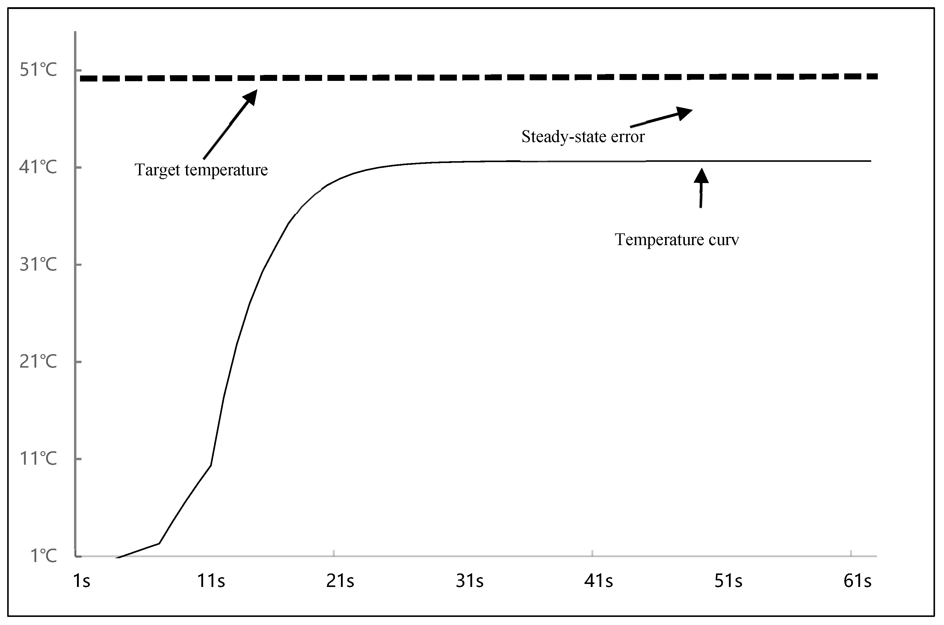
During the initial heating stage, the algorithm employs only proportional control. The temperature control power is adjusted proportionally based on the error magnitude, as given in Equation $U(k)=e(k)\times K_P$.

Where $U(k)$ is the output power at time $k$, $e(k)$ is the error at time $k$, and $K_P$ is the proportional coefficient. According to PID control theory [29,30], when only proportional control is applied, the system reaches steady state quickly but exhibits steady-state errors. The temperature control curve is shown in Figure 3 (Data source: computer simulation). In the figure, the target temperature is set to 50 °C, and only the proportional control method is adopted. As shown in the figure, during the latter stage of the temperature control process, a steady-state error exists between the controlled temperature and the target temperature.

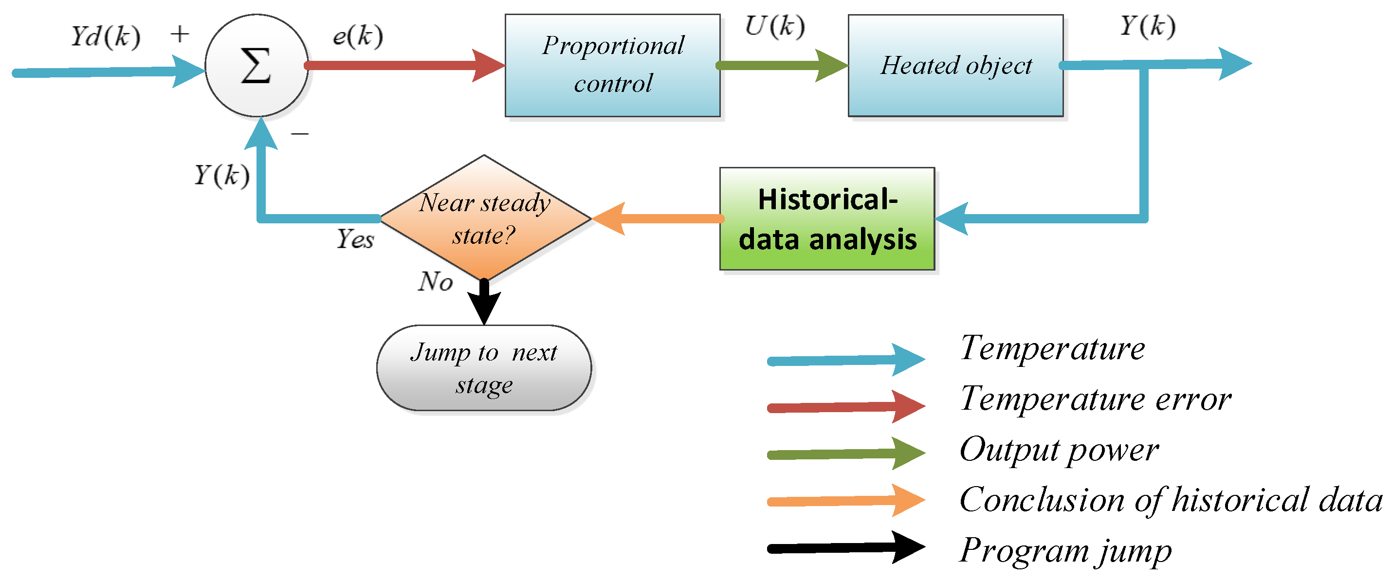
During proportional control, the historical data of the controlled temperature are analyzed to determine whether the temperature is approaching steady state. When the controlled temperature is found to be close to steady state, the control program enters the second stage. The control flow chart for this phase is shown in Figure 4.

In Figure 4, $Yd(k)$ is the target temperature, $Y(k)$ is the current temperature of the heated object at time $k$, $e(k)$ is the error at time $k$, and $U(k)$ is the output power at time $k$. (Throughout this paper, signal type legends in other flowcharts are consistent with those in Figure 4).

3.2. Control Strategy for Pre-Steady Phase

In the rapid heating phase, as the error decreases, the system’s output power becomes increasingly smaller, gradually approaching the heat loss of the heated object. At this point, the heated object is close to thermal equilibrium, so the temperature curve also enters or approaches a steady state. Subsequently, if further temperature increase is required, integral control must be added to enhance the output power. However, this easily causes significant overshoot due to integral windup. To avoid this, the integral value is set to a fixed value during the pre-steady phase. This fixed value is the quotient of the output power at the end of the rapid heating phase and the integral coefficient, which can be obtained from Equation $I=U(k_i)/K_i$. In this equation, $I$ denotes the fixed integral value, $K_i$ is the integral coefficient, and $U(k_i)$ represents the output power at the end of the previous phase. Then, the output power control formula is adjusted to PI mode with a fixed integral value.

$$U(k)=K_P\times e(k)+K_i\times I$$

(8)

The objective is to replace the prior proportional control with constant integral control, while the proportional term continues adjusting power output based on the error between the current and target temperatures. The controlled temperature will then rapidly reach a new steady-state phase. Repeating this process causes the temperature curve to exhibit a stepped pattern. When the error converges to the system’s required accuracy, the control program transitions to the next phase. The controlled temperature curve for this phase is shown in Figure 5a, and the corresponding control flowchart is presented in Figure 5b. The blue dashed arrow signifies the calculated integral value utilized in integral control. Throughout all flowcharts in this article, blue dashed lines adhere to the same legend as specified in this figure.

This strategy effectively eliminates integral windup, avoids excessive overshoot, and ensures rapid temperature rise.

In this phase, the current temperature will be continuously monitored. If the current error approaches the system’s required accuracy, the system will enter the steady-state phase.

3.3. Control Strategy for Steady-State Phase

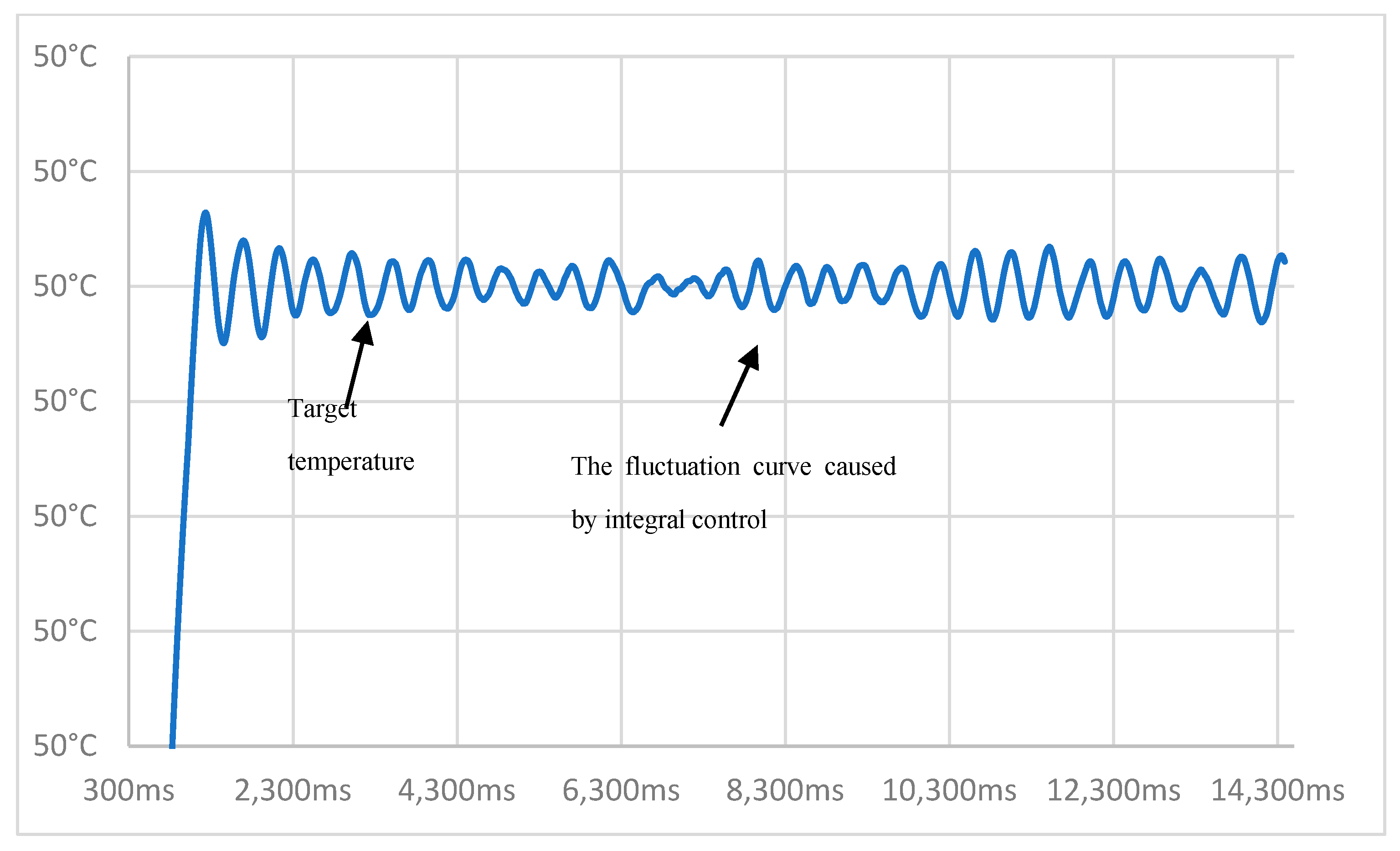
In the steady-state phase, the temperature of the heated object nearly reaches the target value. At this stage, implementing dynamic integral control does not cause excessive overshoot, and introducing derivative control further reduces output power oscillations. The temperature control strategy during this phase is described in Equations (9)–(11).

$$U(k)=K_P\times e(k)+K_i\times I(k)+K_d\times D(k)$$

(9)

$$I(k)=I(k-1)+e(k)$$

(10)

$$D(k)=e(k)-e(k-1)$$

(11)

Here, $D(k)$ is the differential value at time $k$, $K_d$ is the differential coefficient, and $I(k)$ is the integral value at time $k$. During this phase, the integral action becomes the primary factor in regulating the output power. However, due to the time-delay characteristic of the integral action, the temperature control curve will fluctuate around the target value. Figure 6 shows an amplified view of this phase’s behavior.

To overcome the problem of system time delay, we can use the transfer function (Equation (7)) to predict the system’s output state and proactively adjust the integral value based on this prediction, thereby stabilizing the system’s output.

To predict the system state, we need to apply a Z-transform to the transfer function (Equation (7)). The discretized transfer function after transformation is given by Equation (12), where T denotes the sampling period.

$$G(z)=15.5\times {\displaystyle \frac{z^{1-16/T}}{z-e^{-T/155.5}}}$$

(12)

This equation can be transformed into Equation (13).

$${\displaystyle \frac{Y(z)}{U(z)}}=15.5\times {\displaystyle \frac{z^{1-16/T}}{z-e^{-T/155.5}}}$$

(13)

Furthermore, this equation can be transformed into a different form.

$$y(k+1)=15.5u(k+1-16/T)+e^{-T/155.5}y(k)$$

(14)

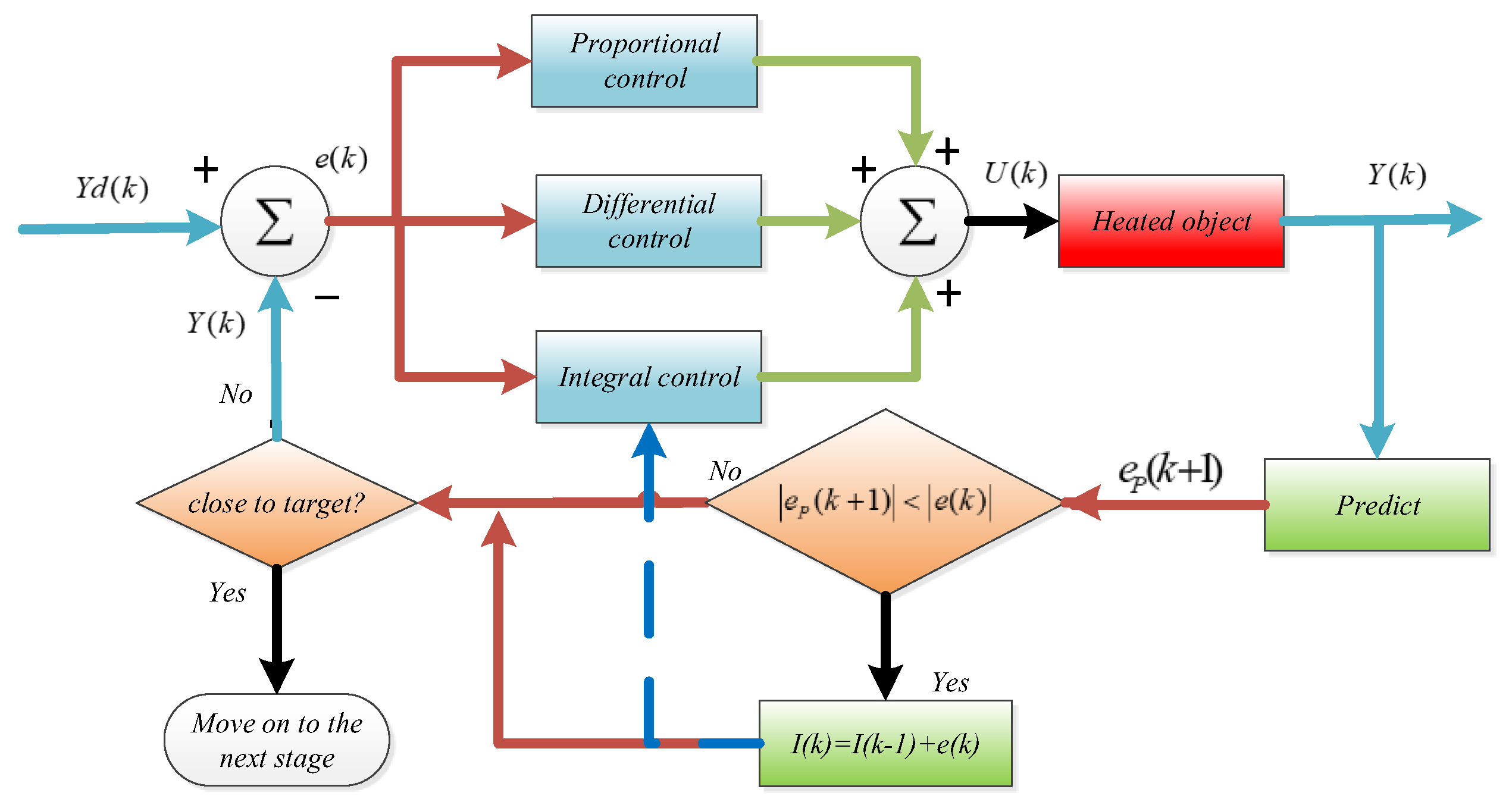
In Equation (14), $y(k)$ is the temperature of the heated object at moment $k$, $u(k)$ is the controller’s output voltage at moment $k$, and $T$ is the sampling period. Equation (14) can be used to predict the system’s output state in the next sampling cycle. At this stage, the following strategy can be adopted to proactively adjust the integral value in PID control: If the predicted error in the next cycle has the same sign as the current cycle’s error and its absolute value decreases, Equation (10) is no longer applied. Thereafter, the integral value remains constant, and the system output is determined by the proportional control component. If the two errors have opposite signs, or if they have the same sign but the next cycle’s error absolute value is greater than or equal to the current cycle’s, Equation (10) continues to be applied. In this case, the system output is primarily influenced by the integral control action.

This adaptive strategy effectively mitigates integral hysteresis effects while accelerating transient convergence. However, system stability tends to be compromised under such dynamic conditions. To enhance regulatory precision, the system may transition to the subsequent control phase characterized by refined parameter adjustments. The corresponding control logic diagram for this advanced phase is shown in Figure 7. In the figure, $e_P(k+1)$ represents the prediction error at the (k + 1)-th moment.

3.4. Control Strategy of Super-Stable Phase

According to the analysis in the previous section, the time delay of the integration effect is one of the reasons for the oscillation of the output power of the standard PID controller. The external environment of the temperature control system is usually stable, so the time delay of the integration effect becomes the main reason affecting temperature control accuracy.

Therefore, this paper proposes a super-stable control strategy to address the delay caused by the integration effect: When the system enters steady state, the integral value is fixed at the average of the peak and valley integral values. The system’s output power is then influenced solely by proportional and differential control, while integral control provides a constant base power. Building on the theoretical foundation established above, the output power control is formulated using Equations (15)–(17), where $I_p$ denotes the integral value at the peak moment and $I_d$ represents the integral value at the valley moment.

$$I(k)=(I_d+I_p)/2$$

(15)

$$D(k)=e(k)-e(k-1)$$

(16)

$$U(k)=K_P\times e(k)+K_i\times I(k)+K_d\times D(k)$$

(17)

If the system is undisturbed, the control effect will be as shown in Figure 8. When the system encounters disturbances (such as wind interference, external temperature fluctuations, etc.), significant fluctuations will recur, and the absolute error will exceed the amplitude of the current peak and valley errors. Under such circumstances, the system can exit the super-stable control phase and revert to the steady-state control phase.

So, the complete control flow of this phase is shown in Figure 9, where $Y_p$ represents the temperature at peak time and $Y_V$ represents the temperature at valley time.

4. Variable Proportional Coefficient Control Based on Output Voltage

The industrial glue dispensing system requires not only rapid convergence and high precision but also good disturbance rejection performance. This means that when disturbances occur, temperature fluctuations should be minimal, the temperature should quickly re-converge, and the system should have a wide range of applicable parameters while being easy to use and adjust. To meet this requirement, a variable-coefficient PID control algorithm based on output voltage is proposed in this paper. This method correlates the coefficients of traditional PID controllers with the output voltage of the temperature control system, ensuring that the system can respond to disturbances in a short period while avoiding excessive oscillations caused by overly large coefficients. To achieve this goal, this article adds a scaling factor α to the PID formula, relates the integral value to the output voltage of two adjacent sampling periods to adjust the sensitivity of the integral effect, and adds the scaling factor $\beta$ to adjust the sensitivity of the proportional control effect. Currently, the temperature control formulas are shown in Equations (18)–(22), where α in Equation (14) and $\beta$ in Equation (16) are adjustable coefficients that can be appropriately adjusted based on the system resolution.

$$U_i=I(k)\times K_i$$

(18)

$$I_x=U(k-1)\times \alpha$$

(19)

$$K_{ix}=U_i/I_x$$

(20)

$$K_{px}=U(k-1)\times \beta$$

(21)

$$U(k)=K_{px}\times e(k)+K_{ix}\times I(k)+K_d\times D(k)$$

(22)

In the formulas, $U_i$ is the output voltage generated by integral control, $I_x$ is the integral value adjusted by factor $\alpha$, $K_{ix}$ is the adjusted integral coefficient, and $K_{px}$ is the proportional coefficient adjusted by $\beta$. According to the above formulas, when the steady-state system is disturbed and the output power increases, a larger proportional coefficient and integral value will be obtained, than changing the sensitivity and strength of the integral control. The difference between this control method and fuzzy PID is that fuzzy PID adjusts the values of PID parameters based on a pre-set fuzzy rule library, errors, and error change rates [21]. While the method in this article adjusts PID parameters based on the output voltage to ensure that the PID adjustment effect is neither too extreme nor too slow. Compared to fuzzy PID, the method proposed in this paper has lower computational complexity and a more sensitive response.

5. Experiment Results and Discussion

In this section, real-time heating tests of the glue dispensing system were conducted to validate the algorithm. Additionally, the performance of this algorithm was compared with the conventional PID adjustment method based on integral anti-windup and fuzzy PID algorithm, to evaluate the proposed method’s performance in terms of overshoot, oscillation period, response time, and parameter applicability range.

5.1. Experiment Setting

In this experiment, a closed-loop temperature control system was developed for an industrial glue dispensing system. The heated assembly consists of a series-connected configuration including a pressure plate, metering machine filling valve, heating module, glue gun copper sleeve, and valve block. Industrial glue flows sequentially through these components, each of which is equipped with a T-type thermocouple. These thermocouples are then interfaced with an external temperature acquisition unit to monitor the real-time surface temperatures of the tested components.

The control system employs a microcontroller-centric embedded platform based on the STM32F030. This system generates Pulse-Width Modulation (PWM) signals with adjustable duty cycles to regulate the switching state of a thyristor power controller, thereby modulating the power delivered to the heating elements.

A 6-channel temperature acquisition module with a 1 kS/s (kilo-samples per second) sampling rate is integrated. This device maintains ±0.1 °C measurement accuracy across the operational temperature range of −100 °C to 400 °C.

The embedded microcontroller is primarily responsible for running temperature control software, collecting temperature values from each thermocouple, and invoking the algorithm proposed in this paper to calculate output power.

The experimental firmware is implemented in the C language, consisting of three core components: a temperature acquisition module, a temperature control algorithm implementation, and an output power regulation module.

During the experimental procedure, the primary focus was placed on monitoring the temperature dynamics of the heating module. Temperature control experiments were initiated under the condition that the module temperature had stabilized and remained below 10 °C. The temperature of each channel of the DUT was required to be sequentially regulated within the specified range of 30 °C to 110 °C. To ensure equipment safety, a 15 V input voltage ceiling is imposed on each heating element. Accordingly, the proposed algorithm restricts output voltage to 0–15 V. Through voltage-to-duty-cycle conversion, this corresponds to a PWM output range of 0–80%. At 0% duty cycle, heat dissipation occurs primarily via gray-body radiation from the tested components.

5.2. PID Parameter Tuning

When manually tuning parameters, there is a method called the Ziegler–Nichols tuning method. Its main approach involves adjusting the system to a critical oscillation state under proportional control only, obtaining the critical gain and oscillation period. Relatively appropriate PID parameters can then be calculated based on these two quantities. Although this method has been widely applied in PID tuning, it suffers from the drawback of difficulty in precisely determining the critical state. The relay auto-tuning method adopted in this paper also induces oscillation in the system first, then calculates suitable PID parameters by measuring peak-to-peak values and oscillation periods, which reflect the inherent characteristics of the system. Its advantage lies in generating the system’s oscillatory state through step signals of the control input, eliminating the need to laboriously seek the critical state.

The steps of this method are as follows:

• Set a temperature, such as 50 °C, as the reference value. When the temperature of the heated object exceeds 50 °C, the control output voltage is set to 0 V; when it falls below 50 °C, the output voltage is set to 5 V. This approach forces the temperature of the heated object to exhibit periodic oscillations. The oscillation period and amplitude directly reflect the inherent characteristics of the heated object.
• Analyze and record the peaks and valleys of the temperature as A, the output voltage as D, and the oscillation period as Pu.
• Then, according to the previous experience, the parameters of PID can be calculated based on

  Table 1. PID Parameter Tuning Table.

  Control Type	Kp	Ki	Kd
  PI	$0.4Ku$	$0.48Ku/Pu$	0
  PID	$0.6Ku$	$1.2Ku/Pu$	$0.075Ku\times Pu$
  Where $Ku=4D/(A\times \pi )$

  .

5.3. System Response Speed Comparison Test

A comparison is made of the differences in overshoot, oscillation period, response time, and parameter applicability between this method, the integral limited PID algorithm, and the fuzzy PID algorithm when implemented on the same hardware device.

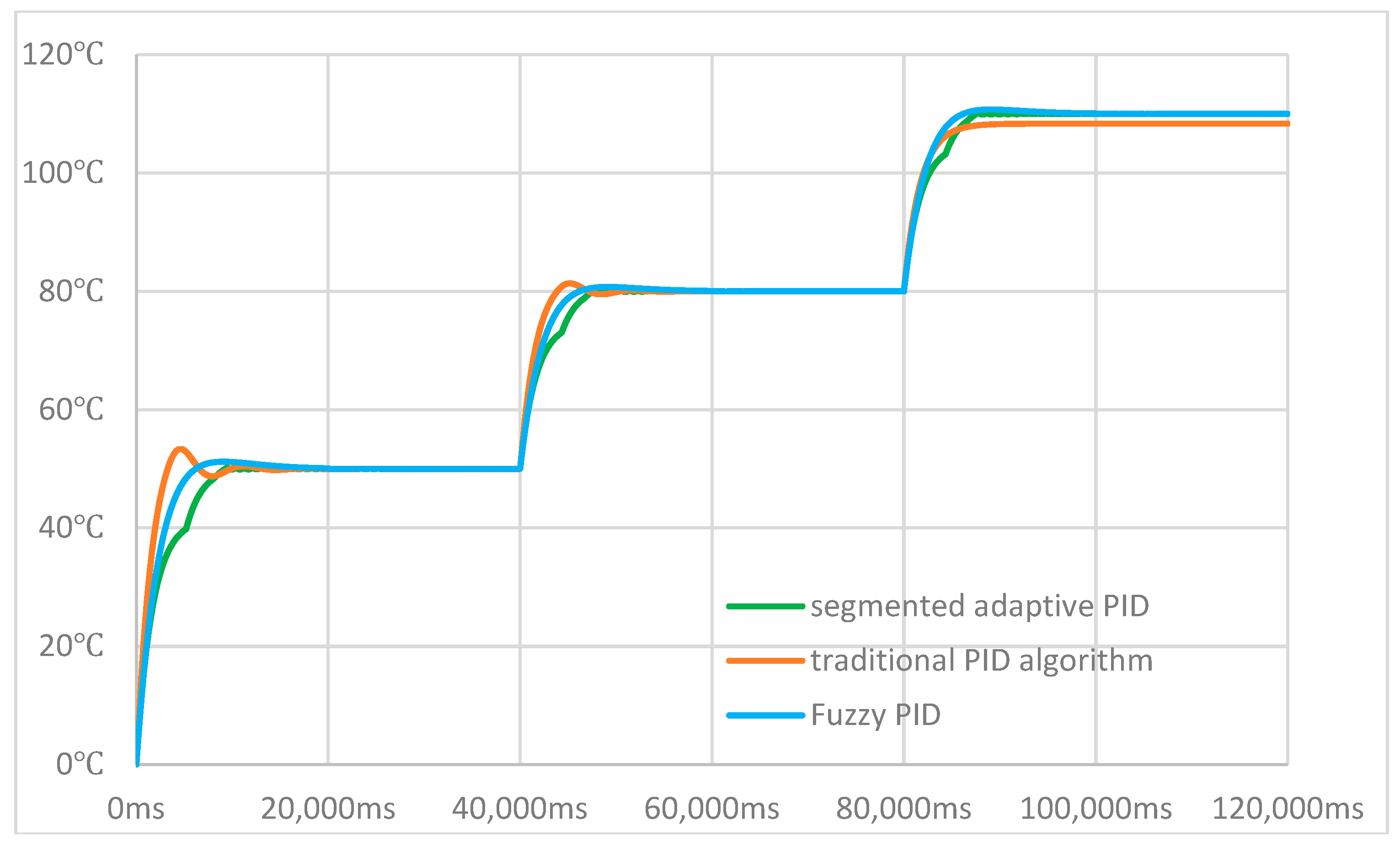
First, heating experiments were conducted to compare and evaluate the heating effect across three temperature ranges: 0 °C to 50 °C, 50 °C to 80 °C, and 80 °C to 110 °C. In these experiments, the traditional PID algorithm limited the integral value to a maximum of 80, whereas the proposed method imposed no such limitation on the PID integral value. The results are shown in Figure 10.

To further test the anti-overshoot performance of the proposed algorithm, integral windup limitation measures were incorporated into the standard PID algorithm. This approach can, to some extent, avoid the overshoot phenomenon caused by excessive integral accumulation. The integral windup limits of the standard PID algorithm were then set to 80 and 50, respectively, and the performance of heating the target from 0 °C to 50 °C was compared with that of the proposed method. The results are shown in Figure 11.

5.4. Disturbance Rejection Test

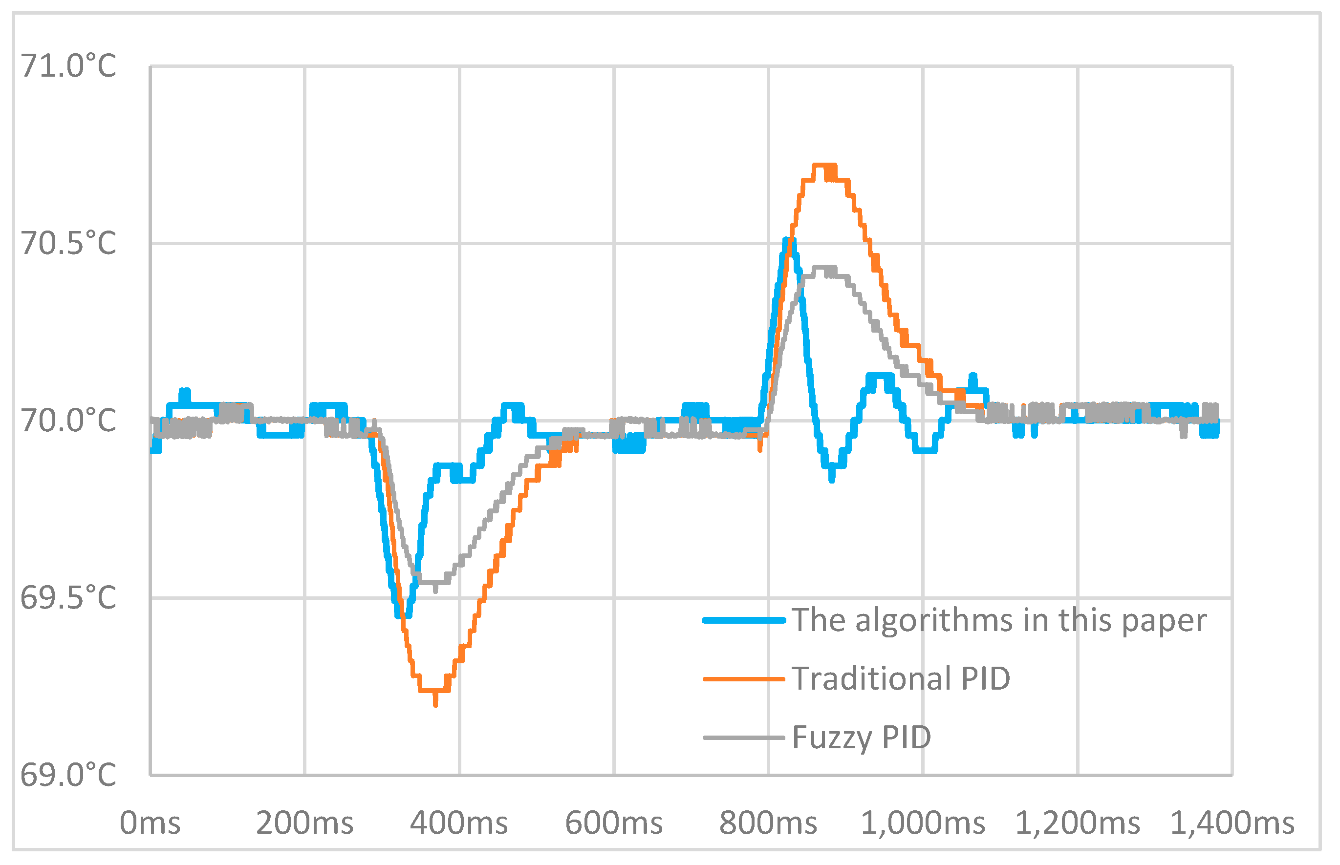
In the experiment, in order to test the disturbance rejection performance, when the temperature of the heated object was stable at 70 °C, a fan was used to directly blow on the heated object. After the temperature of the heated object stabilized again, the fan was turned off to simulate sudden changes in ambient temperature. The amplitude and convergence rate of temperature changes of the heated object under the three methods were measured. The experimental results are shown in Figure 12.

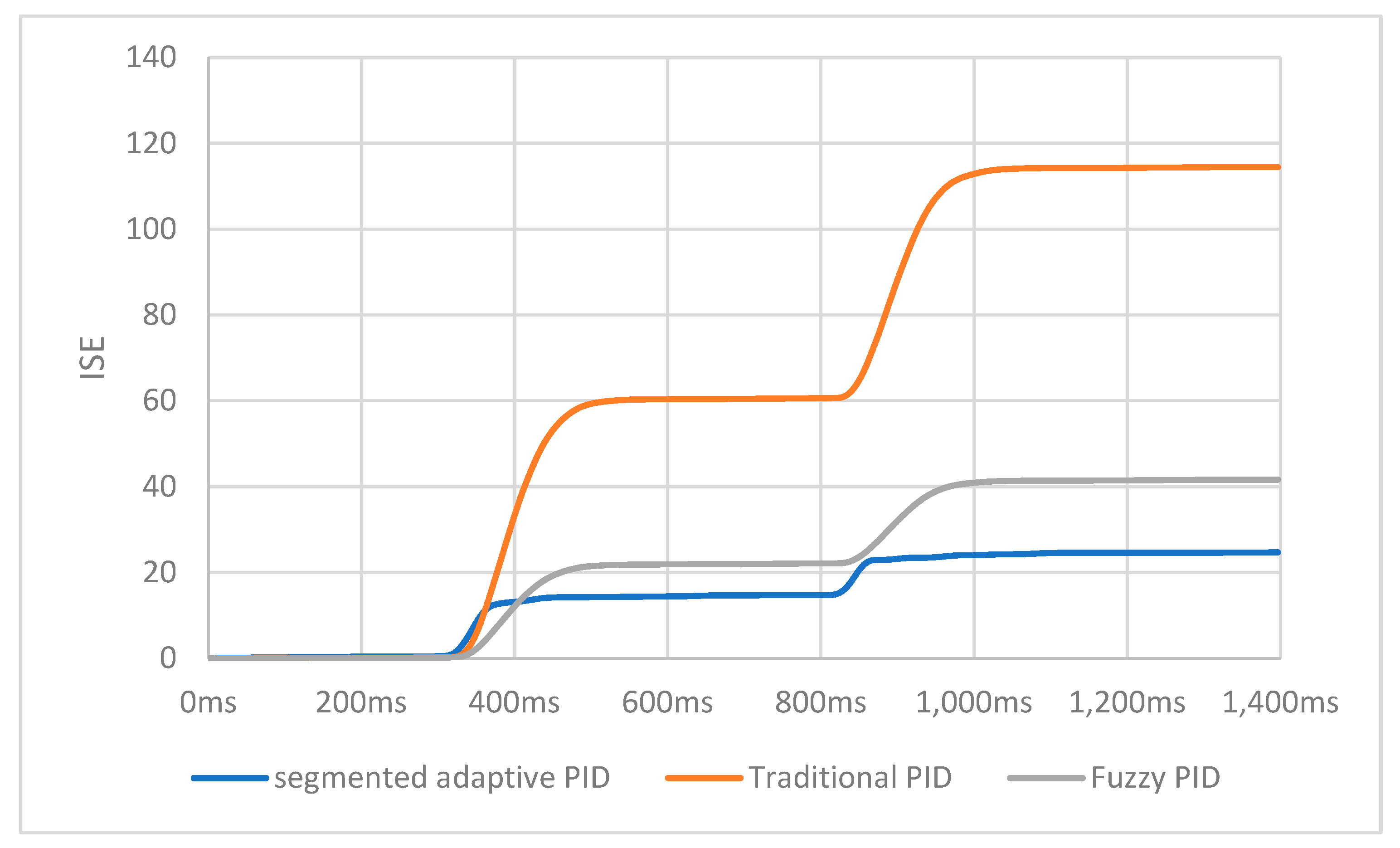
5.5. Performance Test of the ISE (Integral of Squared Error) Index

To further investigate the dynamic response characteristics of the algorithm, ISE index data were statistically analyzed. The ISE at moment k is defined by Equation (1).

$$ISE(k)={\displaystyle {\int }_0^k}{e(k)}^{2}dt$$

(23)

Based on the experimental results in Section 5.4 and combined with Equation (23), the comparison graph of ISE during disturbance is presented in Figure 13.

And based on the experimental results in Section 5.3, the comparison graph of ISE during rapid heating phase, the comparison graph of ISE is presented in Figure 14.

5.6. Discussion

In this study, the proposed temperature control algorithm was verified through a series of heating experiments, and its performance was compared with the traditional PID control method based on the integral anti-windup algorithm and fuzzy PID algorithm. The experimental results show that the new algorithm exhibits significant advantages in multiple key performance indicators.

5.6.1. Overshoot

According to the experimental data, the overshoot of the new algorithm is significantly lower than that of the traditional PID algorithm under different output power conditions. Especially during the temperature rising processes from 0 °C to 50 °C, 50 °C to 80 °C, and 80 °C to 110 °C, the overshoot phenomenon of the traditional PID algorithm is closely related to its integral limit value and heating power. When the integral limit value is set too large, the system will exhibit obvious overshoot. Conversely, when the integral limit value is too small, the heating speed of the system will significantly slow down, and steady-state errors may even occur. In contrast, the new algorithm can maintain a small and stable overshoot at different heating stages, and its anti-overshoot performance is comparable to that of fuzzy PID, indicating that it has a lower demand for parameter adjustment and stronger adaptability.

5.6.2. Disturbance Rejection Performance

To test the disturbance rejection performance of the algorithm, a fan was introduced as a disturbance source when the temperature of the heated object was stabilized at 70 °C. Experimental results show that the maximum error of the new algorithm is only approximately 0.5 °C, and it rapidly converges to within 0.2 °C within 100 sampling periods. Although the maximum error of the new algorithm is slightly larger than that of the fuzzy PID algorithm, its convergence speed is faster. In contrast, the traditional PID algorithm exhibits a maximum error of around 0.8 °C and requires 200 sampling periods to achieve the same convergence accuracy. This indicates that the new algorithm not only outperforms in terms of disturbance rejection amplitude but also demonstrates significant advantages in recovery speed.

5.6.3. Performance Analysis of the ISE

Conclusions drawn from Figure 13 are as follows: The ISE index starts to be calculated from 0 after the system reaches a stable state. When the system is suddenly disturbed, the ISE index of the method proposed in this paper is the smallest, and it shows no significant difference from that of the fuzzy PID method. It can be concluded that the dynamic response characteristics of the method in this paper are the best among the three methods.

However, the following conclusions can be drawn from Figure 14: At the initial stage of heating, the ISE index of the method proposed in this paper is evidently the largest. This indicates that the heating rate of the proposed method during the rapid heating phase is slower than that of the other two methods. However, by synthesizing the analyses of Figure 10 and Figure 11, it can be observed that although the proposed method achieves the pre-set temperature at a slower rate, the duration required to reach the pre-set temperature and attain a steady state is comparable to that of the other two methods, while exhibiting a smaller overshoot. This suggests that the proposed method sacrifices heating rate during the heating phase to obtain reduced overshoot. Given the application context of industrial dispensing systems, where greater emphasis is placed on the stability of temperature control performance, the proposed method is more suitable.

6. Conclusions

This paper proposes a segmented adaptive PID temperature control method applicable to industrial dispensing systems. This method combines a segmented temperature control algorithm with a temperature control algorithm of variable control coefficients based on output power. The experimental results show that, compared with the traditional PID method, under the same experimental conditions, the proposed method reduces the overshoot by 2 to 4 °C, increases the convergence speed by approximately 30%, and decreases the amplitude of temperature fluctuation after interference by about 0.2 °C.

Through the segmented control strategy, this method adopts proportional control in the rapid heating stage, PI control with a fixed integral value in the pre-steady state stage, dynamic integral control and derivative control in the steady state stage, and PID control with a fixed integral value in the super-steady state stage, effectively solving the problems existing in traditional PID control in industrial dispensing systems, such as large overshoot, slow convergence speed, low control accuracy, and poor anti-interference ability.

In addition, this paper also proposes a variable proportional coefficient control method based on output power. By adjusting the PID control parameters, the system can respond to interference within a short time while avoiding excessive oscillation caused by an overly large coefficient. This method has a low computational complexity and is more responsive.

Meanwhile, the performance of this algorithm in terms of overshoot and convergence speed is comparable to that of fuzzy PID. However, fuzzy PID requires pre-designing complex fuzzy rules by integrating expert experience. In contrast, this algorithm simplifies programming design to some extent and reduces excessive dependence on expert experience.

In conclusion, the segmented adaptive PID temperature control method proposed in this paper exhibits good control performance and application prospects in industrial dispensing systems, providing an effective solution for improving the temperature control accuracy and stability of industrial dispensing systems.

References

- Ang, K.H.; Chong, G.; Li, Y. PID control system analysis, design, and technology. IEEE Trans. Control Syst. Technol. 2005, 13, 559–576. [Google Scholar]
- Zhang, P.; Yuan, M.; Wang, H. Self-Tuning PID Based on Adaptive Genetic Algorithms with the Application of Activated Sludge Aeration Process. In Proceedings of the 2006 6th World Congress on Intelligent Control and Automation, Dalian, China, 21–23 June 2006; pp. 9327–9330. [Google Scholar]
- Ziegler, J.G.; Nichols, N.B. Optimum Settings for Automatic Controllers. J. Fluids Eng. 1942, 64, 759–765. [Google Scholar] [CrossRef]
- Åström, K.; Hägglund, T. Revisiting the Ziegler–Nichols step response method for PID control. J. Process. Control 2004, 14, 635–650. [Google Scholar] [CrossRef]
- Wang, Q.-G.; Zhang, Z.; Astrom, K.J.; Zhang, Y.; Zhang, Y. Guaranteed Dominant Pole Placement with PID Controllers. IFAC Proc. Vol. 2008, 41, 5842–5845. [Google Scholar] [CrossRef]
- Shahiri, M.; Ranjbar, A.; Karami, M.R.; Ghaderi, R. New tuning design schemes of fractional complex-order PI controller. Nonlinear Dyn. 2016, 84, 1813–1835. [Google Scholar] [CrossRef]
- Gude, J.J.; Kahoraho, E. Kappa-tau type PI tuning rules for specified robust levels. IFAC Proc. Vol. 2012, 45, 589–594. [Google Scholar] [CrossRef]
- Selvi, J.A.V.; Radhakrishnan, T.; Sundaram, S. Performance assessment of PID and IMC tuning methods for a mixing process with time delay. ISA Trans. 2007, 46, 391–397. [Google Scholar] [CrossRef]
- Nath, U.M.; Dey, C.; Mudi, R.K. Review on IMC-based PID Controller Design Approach with Experimental Validations. IETE J. Res. 2021, 69, 1640–1660. [Google Scholar] [CrossRef]
- Zhang, W.; Yang, M. Comparison of auto-tuning methods of PID controllers based on models and closed-loop data. In Proceedings of the 2014 33rd Chinese Control Conference (CCC), Nanjing, China, 28–30 July 2014; pp. 3661–3667. [Google Scholar]
- Sanchez-Palma, J.; Ordonez-Avila, J.L. A PID Control Algorithm With Adaptive Tuning Using Continuous Artificial Hydrocarbon Networks for a Two-Tank System. IEEE Access 2022, 10, 114694–114710. [Google Scholar] [CrossRef]
- Wu, X.; Wu, J.; Li, D. Designation and Simulation of Environment Laboratory Temperature Control System Based on Adaptive Fuzzy PID. In Proceedings of the 2018 IEEE 3rd Advanced Information Technology, Electronic and Automation Control Conference (IAEAC), Chongqing, China, 12–14 October 2018; pp. 583–587. [Google Scholar]
- Xin, H.; Huang, T.; Liu, X.; Tang, X. Temperature Control System Based on Fuzzy Self-Adaptive PID Controller. In Proceedings of the 2009 3rd International Conference on Genetic and Evolutionary Computing (WGEC), Guilin, China, 14–17 October 2009; pp. 537–540. [Google Scholar]
- Hu, L.; Wang, W.; Wang, Z. Research on Temperature Control Method of Variable Structure Thermoelectric Furnace Based on Fuzzy PID Optimized by Genetic Algorithm. In Proceedings of the 2022 2nd International Conference on Electrical Engineering and Control Science (IC2ECS), Nanjing, China, 16–18 December 2022; pp. 716–720. [Google Scholar]
- Lafont, F.; Balmat, J.F. Optimized fuzzy control of a greenhouse. Fuzzy Sets Syst. 2002, 128, 47–59. [Google Scholar] [CrossRef]
- Chen, L.; Du, S.; He, Y.; Liang, M.; Xu, D. Robust model predictive control for greenhouse temperature based on particle swarm optimization. Inf. Process. Agric. 2018, 5, 329–338. [Google Scholar] [CrossRef]
- Pei, X.; Zhang, J.; Jia, W.; Han, D.; Ma, S.; Xu, B. Research on Junction Temperature Control Method of LED Array. In Proceedings of the 2024 4th International Conference on Electrical Engineering and Mechatronics Technology (ICEEMT), Hangzhou, China, 5–7 July 2024; pp. 166–170. [Google Scholar]
- Wu, T.-Y.; Jiang, Y.-Z.; Su, Y.-Z.; Yeh, W.-C. Using Simplified Swarm Optimization on Multiloop Fuzzy PID Controller Tuning Design for Flow and Temperature Control System. Appl. Sci. 2020, 10, 8472. [Google Scholar] [CrossRef]
- Jiang, X.; Cheng, T. Design of a BP neural network PID controller for an air suspension system by considering the stiffness of rubber bellows. Alex. Eng. J. 2023, 74, 65–78. [Google Scholar] [CrossRef]
- Hanna, Y.F.; Khater, A.A.; El-Bardini, M.; El-Nagar, A.M. Real time adaptive PID controller based on quantum neural network for nonlinear systems. Eng. Appl. Artif. Intell. 2023, 126, 106952. [Google Scholar] [CrossRef]
- Zhang, R.; Gao, L. The Brushless DC motor control system Based on neural network fuzzy PID control of power electronics technology. Optik 2022, 271, 169879. [Google Scholar] [CrossRef]
- Dai, B.; Chen, R.; Chen, R.-C. Temperature control with fuzzy neural network. In Proceedings of the 2017 IEEE 8th International Conference on Awareness Science and Technology (iCAST), Taichung, Taiwan, 8–10 November 2017; pp. 452–455. [Google Scholar]
- He, Y.; Jin, X.; Jin, P.; Su, J.; Li, F.; Lu, H. Temperature Control Performance Improvement of High-Power Laser Diode with Assistance of Machine Learning. Photonics 2025, 12, 241. [Google Scholar] [CrossRef]
- Mureşan, V.; Abrudean, M.; Ungureşan, M.L.; Clitan, I.; Sita, V.; Coloşi, T. Intelligent Temperature Control in an Industrial Furnace. In Proceedings of the ICCAE 2020: 2020 12th International Conference on Computer and Automation Engineering, Sydney, NSW, Australia, 14–16 February 2020. [Google Scholar]
- Xu, Z.; Liu, J. Research on Temperature Control of Liposome High Pressure Homogenizer Based on Genetic Algorithm Optimization PID. Procedia Comput. Sci. 2022, 208, 330–337. [Google Scholar] [CrossRef]
- Corradini, L.; Costabeber, A.; Mattavelli, P.; Saggini, S. Parameter-Independent Time-Optimal Digital Control for Point-of-Load Converters. IEEE Trans. Power Electron. 2009, 24, 2235–2248. [Google Scholar] [CrossRef]
- Ren, K.; Xie, Y.; Wang, C.; Yan, J.; Shi, Y.; Guo, J.; Guo, J. Application of the fuzzy proportional integral differential (PID) temperature control algorithm in a liver function test system based on a centrifugal microfluidic device. Talanta 2023, 268, 125330. [Google Scholar] [CrossRef]
- Xiao, Y.; Yin, S.; Zhao, Y.; Chen, Y.; Wan, F. Research on the Control Strategy of Battery Roller Press Deflection Device by Introducing Genetic Algorithm to Optimize Integral Separation PID. IEEE Access 2022, 10, 100878–100894. [Google Scholar] [CrossRef]
- Frank, P.; Heger, F.; Heintz, T.; Härtel, H. Computer Aided Adjustment of PID Control for Steam Turbines. IFAC Proc. Vol. 1979, 12, 573–578. [Google Scholar] [CrossRef]
- Buzruk, M.; Ghogare, S.; Deshpande, A. A Novel Maximum Power Point Tracking Control Without Steady State Oscillations Using Extremum Seeking Control Algorithm. In Proceedings of the 2021 Seventh Indian Control Conference (ICC), Mumbai, India, 20–22 December 2021; pp. 259–264. [Google Scholar]