
CNN-Assisted Effective Radar Active Jamming Suppression in Ultra-Low Signal-to-Jamming Ratio Conditions Using Bandwidth Enhancement


Abstract
1. Introduction
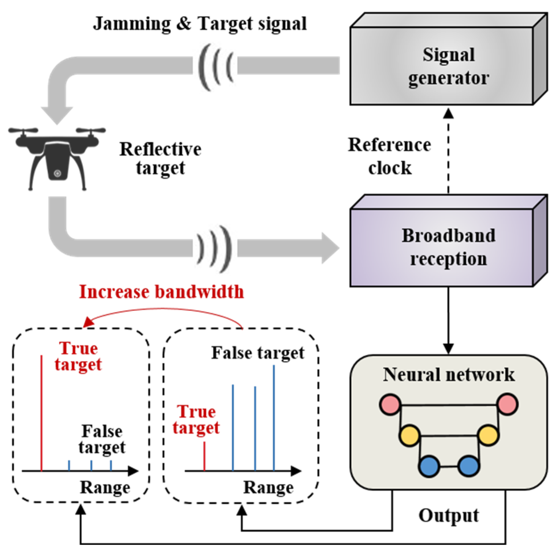
2. Methodology
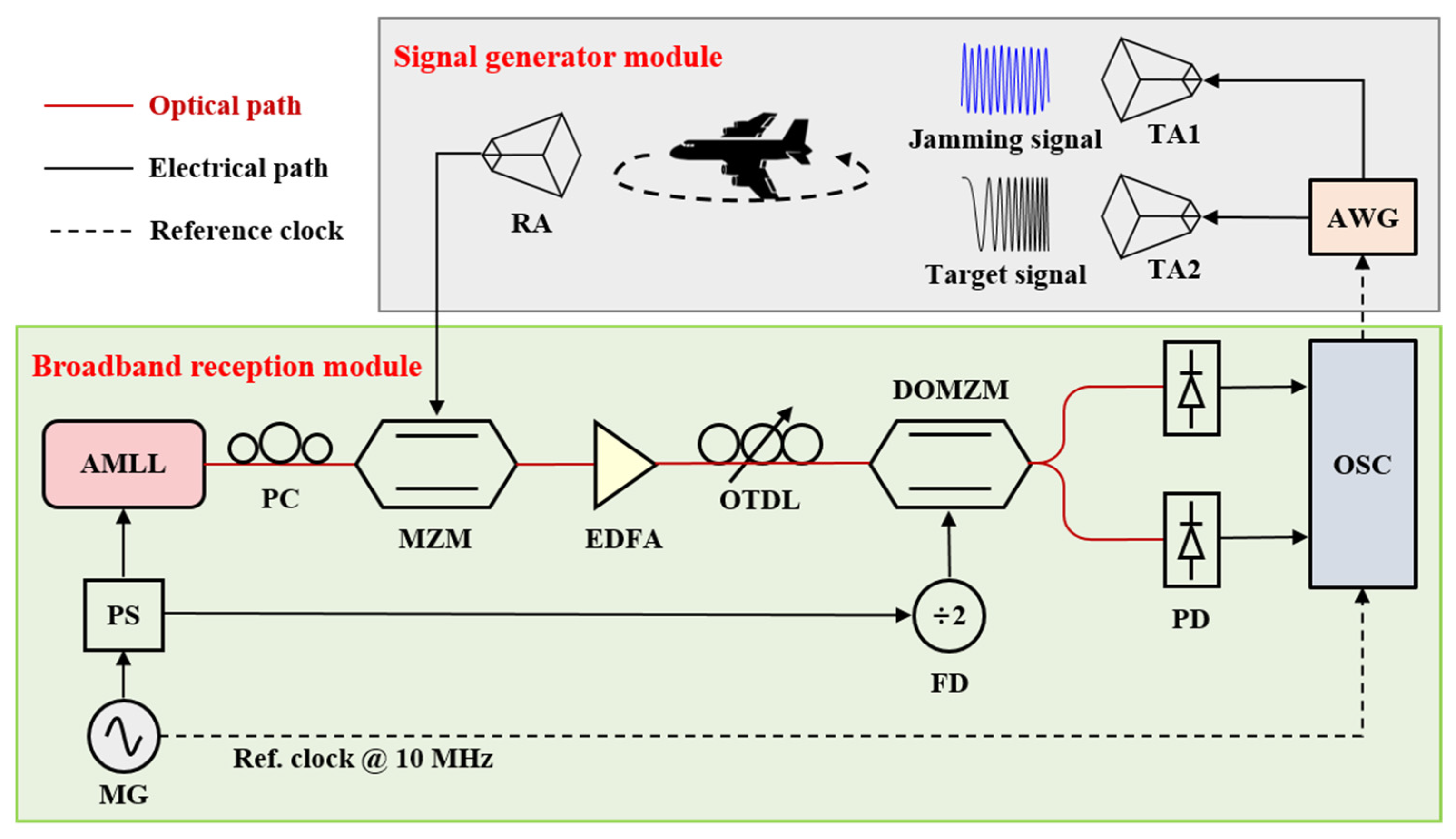
3. Experimental Setup
3.1. Signal Generator Module
3.2. Broadband Reception Module
3.3. CNN Module
4. Results and Discussion
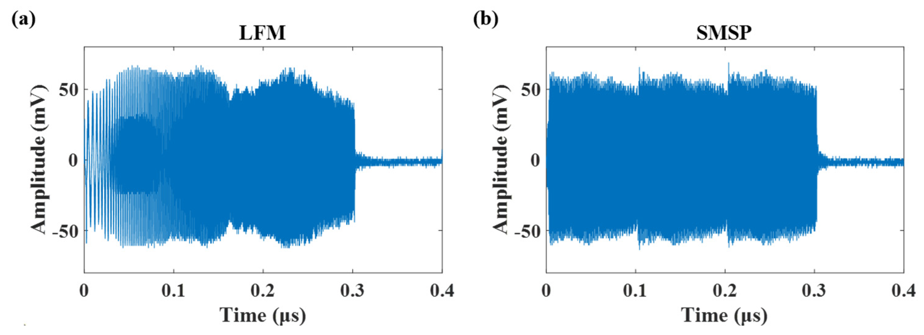
4.1. Results of Pulse Compression
4.2. Results of CNN
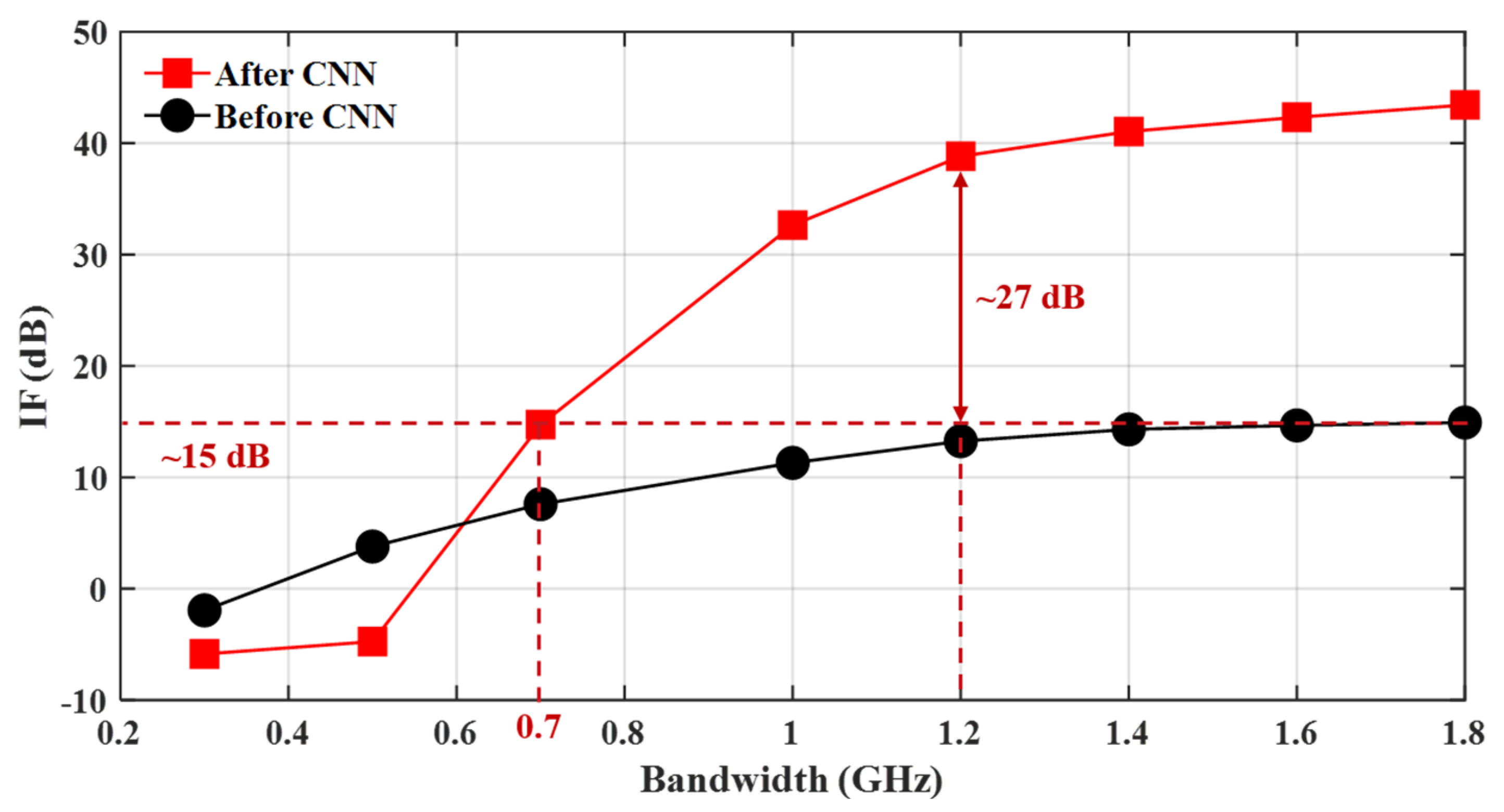
4.3. Comparison of Pulse Compression and CNN
4.4. Results of Time-Frequency Domain
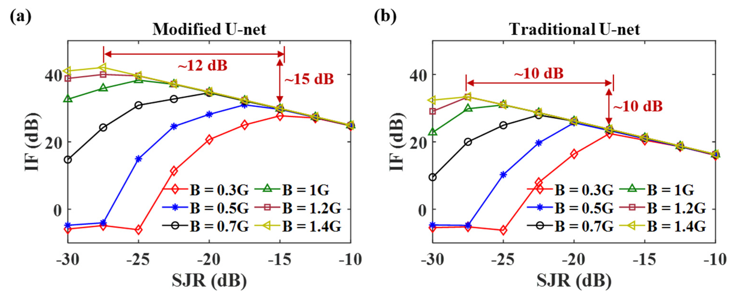
4.5. Comparison of Results with Traditional U-Net
5. Conclusions
Author Contributions
Funding
Data Availability Statement
Conflicts of Interest
References
- Qu, Q.; Wei, S.; Liu, S.; Liang, J.; Shi, J. JRNet: Jamming recognition networks for radar compound suppression jamming signals. IEEE Trans. Veh. Technol. 2020, 69, 15035–15045. [Google Scholar] [CrossRef]
- Calatrava, H.; Tang, S.; Closas, P. Advances in Anti-Deception Jamming Strategies for Radar Systems: A Survey. arXiv 2025, arXiv:2503.00285. [Google Scholar]
- Li, N.; Zhang, Y. A survey of radar ECM and ECCM. IEEE Trans. Aerosp. Electron. Syst. 1995, 31, 1110–1120. [Google Scholar]
- Lan, L.; Xu, J.; Liao, G.; Zhang, Y.; Fioranelli, F.; So, H.C. Suppression of mainbeam deceptive jammer with FDA-MIMO radar. IEEE Trans. Veh. Technol. 2020, 69, 11584–11598. [Google Scholar] [CrossRef]
- Tian, D.; Wang, C.; Ren, W.; Liang, Z.; Liu, Q. ECCM scheme for countering main-lobe interrupted sampling repeater jamming via signal reconstruction and mismatched filtering. IEEE Sens. J. 2023, 23, 13261–13271. [Google Scholar] [CrossRef]
- Liu, Z.; Liao, G.; Yang, Z. Time variant RFI suppression for SAR using iterative adaptive approach. IEEE Geosci. Remote Sens. Lett. 2013, 10, 1424–1428. [Google Scholar] [CrossRef]
- Zhou, F.; Tao, M.; Bai, X.; Liu, J. Narrow-band interference suppression for SAR based on independent component analysis. IEEE Trans. Geosci. Remote Sens. 2013, 51, 4952–4960. [Google Scholar] [CrossRef]
- Li, N.; Lv, Z.; Guo, Z.; Zhao, J. Time-domain notch filtering method for pulse RFI mitigation in synthetic aperture Radar. IEEE Geosci. Remote Sens. Lett. 2021, 19, 4013805. [Google Scholar] [CrossRef]
- Fu, Z.; Zhang, H.; Zhao, J.; Li, N.; Zheng, F. A modified 2-D notch filter based on image segmentation for RFI mitigation in synthetic aperture radar. Remote Sens. 2023, 15, 846. [Google Scholar] [CrossRef]
- Zhao, J.; Liao, G.; Xing, H.; Jia, B.; Liu, S.; Wang, Y.; Zhang, X. Range-frequency domain iterative notch filtering method for RFI mitigation in SAR. IEEE Geosci. Remote Sens. Lett. 2024, 21, 4010305. [Google Scholar] [CrossRef]
- Wang, Z.; Li, J.; Yu, W.; Luo, Y.; Zhao, Y.; Yu, Z. Energy function-guided histogram analysis for interrupted sampling repeater jamming suppression. Electron. Lett. 2023, 59, e12778. [Google Scholar] [CrossRef]
- Abdalla, A.; Ramadan, M.; Liao, Y.; Zhou, S. An adaptive filtering algorithm in pulse-doppler radar for counteracting range-velocity jamming. Int. J. Electron. 2022, 109, 1695–1713. [Google Scholar] [CrossRef]
- Xu, W.; Xing, W.; Fang, C.; Huang, P.; Tan, W. RFI suppression based on linear prediction in synthetic aperture radar data. IEEE Geosci. Remote Sens. Lett. 2021, 18, 2127–2131. [Google Scholar] [CrossRef]
- Li, N.; Lv, Z.; Guo, Z. Observation and mitigation of mutual RFI between SAR satellites: A case study between Chinese GaoFen-3 and European Sentinel-1A. IEEE Geosci. Remote Sens. Lett. 2022, 60, 5112819. [Google Scholar] [CrossRef]
- Zhou, F.; Wu, R.; Xing, M.; Bao, Z. Eigensubspace-based filtering with application in narrow-band interference suppression for SAR. IEEE Geosci. Remote Sens. Lett. 2007, 4, 75–79. [Google Scholar] [CrossRef]
- Feng, J.; Zheng, H.; Deng, Y.; Gao, D. Application of subband spectral cancellation for SAR narrow-band interference suppression. IEEE Geosci. Remote Sens. Lett. 2012, 9, 190–193. [Google Scholar] [CrossRef]
- Zhang, S.; Xing, M.; Guo, R.; Zhang, L.; Bao, Z. Interference suppression algorithm for SAR based on time–frequency transform. IEEE Trans. Geosci. Remote Sens. 2011, 49, 3765–3779. [Google Scholar] [CrossRef]
- Minar, M.R.; Naher, J. Recent advances in deep learning: An overview. arXiv 2018, arXiv:1807.08169. [Google Scholar]
- Gao, S.; Yang, X.; Lan, T.; Han, B.; Sun, H.; Yu, Z. Radar main-lobe jamming suppression and identification based on robust whitening blind source separation and convolutional neural networks. IET Radar Sonar Navig. 2022, 16, 552–563. [Google Scholar] [CrossRef]
- Hua, Q.; Zhang, Y.; Wei, C.; Ji, Z.; Jiang, Y.; Wang, Y.; Xu, D. A self-supervised method based on CV-MUNet++ for active jamming suppression in SAR images. IEEE Trans. Geosci. Remote Sens. 2023, 61, 5209516. [Google Scholar] [CrossRef]
- Jiang, Y.; Yang, Y.; Zhang, W.; Guo, L. Deep learning-based active jamming suppression for radar main lobe. IET Signal Process. 2024, 2024, 3179667. [Google Scholar] [CrossRef]
- Shang, S.; He, K.; Wang, Z.; Yang, T.; Liu, M.; Li, X. Sea clutter suppression method of HFSWR based on RBF neural network model optimized by improved GWO algorithm. Comput. Intell. Neurosci. 2020, 2020, 8842390. [Google Scholar] [CrossRef] [PubMed]
- Shen, H.; George, D.; Huerta, E.; Zhao, Z. Denoising gravitational waves with enhanced deep recurrent denoising auto-encoders. In Proceedings of the ICASSP 2019—2019 IEEE International Conference on Acoustics, Speech and Signal Processing (ICASSP), Brighton, UK, 12–17 May 2019; pp. 3237–3241. [Google Scholar]
- Liu, X.; Zhang, T.; Shi, Q.; Yu, X.; Cui, G.; Kong, L. LPI radar waveform design with desired cyclic spectrum and pulse compression properties. IEEE Trans. Veh. Technol. 2023, 72, 6789–6793. [Google Scholar] [CrossRef]
- Yang, Z.; Du, W.; Liu, Z.; Liao, G. WBI suppression for SAR using iterative adaptive method. IEEE J. Sel. Top. Appl. Earth Observ. 2016, 9, 1008–1014. [Google Scholar] [CrossRef]
- Zeng, L.; Chen, H.; Zhang, Z.; Liu, W.; Wang, Y.; Ni, L. Cutting compensation in the time-frequency domain for smeared spectrum jamming suppression. Electronics 2022, 11, 1970. [Google Scholar] [CrossRef]
- Ronneberger, O.; Fischer, P.; Brox, T. U-Net: Convolutional networks for biomedical image segmentation. In Proceedings of the Medical image computing and computer-assisted intervention–MICCAI 2015: 18th international conference, Munich, Germany, 5–9 October 2015; pp. 234–241. [Google Scholar]
- Huang, G.; Liu, Z.; Van Der Maaten, L.; Weinberger, K.Q. Densely connected convolutional networks. In Proceedings of the IEEE Conference on Computer Vision and Pattern Recognition (CVPR), Honolulu, HI, USA, 21–26 July 2017; pp. 4700–4708. [Google Scholar]
- Giustiniano, D.; Schalch, M.; Liechti, M.; Lenders, V. Interference Suppression in Bandwidth Hopping Spread Spectrum Communications. In Proceedings of the 11th ACM Conference on Security & Privacy in Wireless and Mobile Networks (WiSec’18), Stockholm, Sweden, 18–20 June 2018; pp. 134–143. [Google Scholar]
- Fang, F.; Tian, Y.; Dai, D.; Xing, S. Synthetic aperture radar radio frequency interference suppression method based on fusing segmentation and inpainting networks. Remote Sens. 2024, 16, 1013. [Google Scholar] [CrossRef]
- Yang, G.; Zou, W.; Yu, L.; Chen, J. Influence of the sampling clock pulse shape mismatch on channel-interleaved photonic analog-to-digital conversion. Opt. Lett. 2018, 43, 3530–3533. [Google Scholar] [CrossRef]


| Method | ICA | ESP | This Work |
|---|---|---|---|
| IF (dB) | 4.25 | 8.51 | 16.86 |
Disclaimer/Publisher’s Note: The statements, opinions and data contained in all publications are solely those of the individual author(s) and contributor(s) and not of MDPI and/or the editor(s). MDPI and/or the editor(s) disclaim responsibility for any injury to people or property resulting from any ideas, methods, instructions or products referred to in the content. |
© 2025 by the authors. Licensee MDPI, Basel, Switzerland. This article is an open access article distributed under the terms and conditions of the Creative Commons Attribution (CC BY) license (https://creativecommons.org/licenses/by/4.0/).
Share and Cite
Zhang, L.; Zou, X.; Xu, S.; Chai, M.; Lu, W.; Lv, Z.; Zou, W. CNN-Assisted Effective Radar Active Jamming Suppression in Ultra-Low Signal-to-Jamming Ratio Conditions Using Bandwidth Enhancement. Electronics 2025, 14, 2296. https://doi.org/10.3390/electronics14112296
Zhang L, Zou X, Xu S, Chai M, Lu W, Lv Z, Zou W. CNN-Assisted Effective Radar Active Jamming Suppression in Ultra-Low Signal-to-Jamming Ratio Conditions Using Bandwidth Enhancement. Electronics. 2025; 14(11):2296. https://doi.org/10.3390/electronics14112296
Chicago/Turabian StyleZhang, Linbo, Xiuting Zou, Shaofu Xu, Mengmeng Chai, Wenbin Lu, Zhenbin Lv, and Weiwen Zou. 2025. "CNN-Assisted Effective Radar Active Jamming Suppression in Ultra-Low Signal-to-Jamming Ratio Conditions Using Bandwidth Enhancement" Electronics 14, no. 11: 2296. https://doi.org/10.3390/electronics14112296
APA StyleZhang, L., Zou, X., Xu, S., Chai, M., Lu, W., Lv, Z., & Zou, W. (2025). CNN-Assisted Effective Radar Active Jamming Suppression in Ultra-Low Signal-to-Jamming Ratio Conditions Using Bandwidth Enhancement. Electronics, 14(11), 2296. https://doi.org/10.3390/electronics14112296