Alzheimer’s Disease Detection from Speech Using Shapley Additive Explanations for Feature Selection and Enhanced Interpretability

Abstract

Smart cities provide an ideal framework for the integration of advanced healthcare applications, such as early Alzheimer’s Disease (AD) detection that is essential to facilitate timely interventions and slow its progression. In this context, speech analysis, combined with Artificial Intelligence (AI) techniques, has emerged as a promising approach for the automatic detection of AD, as vocal biomarkers can provide valuable indicators of cognitive decline. The proposed approach focuses on two key goals: minimizing computational overhead while maintaining high accuracy, and improving model interpretability for clinical usability. To enhance efficiency, the framework incorporates a data quality method that removes unreliable speech segments based on duration thresholds and applies Shapley Additive Explanations (SHAP) to select the most influential acoustic features. SHAP is also used to improve interpretability by providing global and local explanations of model decisions. The final model, that is based on Extreme Gradient Boosting (XGBoost), achieves an F1-Score of 0.7692 on the ADReSS dataset, showing good performance and a satisfactory level of clinical utility. This work highlights the potential of explainable AI to bridge machine learning techniques with clinically meaningful insights in the domain of AD detection from speech.

1. Introduction

Smart cities, defined as urban environments that employ digital technology and data collection to improve residents’ quality of life, provide an ideal framework for the integration of advanced healthcare solutions [1]. This way, smart cities can enable early and non-invasive screening for a range of medical conditions through everyday interactions, such as virtual assistants. This approach not only enhances early diagnosis and intervention but also promotes inclusive healthcare by reaching individuals who may not regularly access traditional medical services. A prominent healthcare application that can benefit from the convergence of smart city infrastructure and Artificial Intelligence (AI) is the detection of Alzheimer’s Disease (AD) based on speech analysis and AI techniques, which constitutes the focus of this work.

Alzheimer’s Disease is a neurodegenerative condition characterized by a progressive and often gradual decline in cognitive function, and it stands out as the most common form of dementia, accounting for around 60-70% of all cases [2]. AD manifests through behavioral and personality changes, cognitive decline, and memory loss [2]. This age-related disease is projected to become increasingly prevalent due to demographic shifts that lead to substantial growth in the elderly population. By 2030, one in six people worldwide will be aged 60 or older, increasing from 1 billion in 2020 to 1.4 billion. By 2050, this demographic is expected to double to 2.1 billion, with the population of those aged 80 and older projected to triple from 2020 to 2050, reaching 426 million [3]. In addition, current diagnostic methods are both time-consuming and costly, contributing to the fact that nearly half of those living with AD do not receive timely diagnoses [4]. Given this, there is an urgent necessity for cost-effective and scalable methods to detect even the most subtle forms of AD [5].

One of the hallmarks of AD is the loss of function of neurons, which in turn miss connections with other neurons and die [6]. As a consequence, among the earliest signs of AD is the deterioration in language and speech production [7]. In fact, the capacity for speech and language is a well-established early indicator of cognitive deficits, making it a vital tool in health monitoring and AD detection [8,9]. In this context, several studies highlight many benefits of speech biomarkers for AD detection: they offer ecologically valid assessments during everyday activities, reduce repeated assessment effects and interrater variability, save time and expense, enable remote testing, improve accessibility, and allow frequent testing with richer and more detailed data [10,11,12]. Moreover, Machine Learning (ML) techniques can effectively exploit the information encoded within these speech biomarkers, thereby providing a powerful framework for the development of diagnostic support systems for AD and their integration in smart cities platform.

The deployment of ML-based systems in real-world healthcare applications faces significant challenges, such as restricted availability of annotated datasets and limitations in computational resources. In this scenario, traditional ML models are frequently preferred over computationally intensive Deep Learning (DL) approaches due to their comparatively lower labeled data and resource demands. Additionally, two effective strategies can enhance system performance while minimizing computational overhead: selecting high-quality data for model training [13] and employing feature selection techniques to identify the most relevant features for the task at hand [14].

No less important, for applications in sensitive areas like healthcare, interpretability is a critical factor. While complex models such as DL architectures often yield high accuracy, their decision-making processes can be opaque, leading to a lack of trust and understanding among practitioners. To mitigate this, Explainable Artificial Intelligence (XAI) techniques such as Mutual Information (MI) [15] and Shapley Additive Explanations (SHAP) [16] are increasingly employed to shed light on how features contribute to model predictions. This transparency is vital not only for gaining trust among clinicians and stakeholders but also for improving the model’s robustness and identifying potential biases in the data. Ultimately, enhancing interpretability ensures that ML models can be safely and reliably integrated into sensitive decision-making processes, such as AD detection from speech.

In this work, we have developed an ML-based system capable of detecting Alzheimer’s Disease from spontaneous speech, taking advantage of the distinctive features that voice can reveal about cognitive impairment. This system is based on the Extreme Gradient Boosting (XGBoost) model and exclusively uses the speech modality as input. To address the challenges in the early diagnosis of Alzheimer’s disease mentioned above, this research has focused on two key objectives. Firstly, we have sought to optimize the system to reduce its computational cost by means of the selection of the most reliable speech segments and acoustic features, ensuring that efficiency and hit rates are not compromised. To this end, we have proposed a method for selecting the most reliable speech segments based on their duration, alongside the use of SHAP values to identify the most relevant acoustic features, showing superior performance in comparison to the conventional MI criterion. Secondly, we have aimed to enhance the interpretability of the model, facilitating its practical application in clinical settings. Specifically, we have employed SHAP values to provide both, a deeper insight of the underlying mechanisms of the global model and explanations for model decisions on particular cases. Therefore, we have proposed to adopt SHAP values for a dual purpose: feature selection and model interpretability.

The rest of the paper is organized as follows. Section 2 looks over the state of the art of AD detection from speech. In Section 3, the dataset and the evaluation metrics utilized in the experimentation are described. In Section 4, we present the methodology that we have followed in our research. Section 5 contains the experiments and results that are discussed in Section 6. Finally, in Section 7, we express our conclusions and some lines of future work.

2. Related Work

AD can cause alterations in the physical aspects of voice, including decreased articulatory precision and speech fluency, that degrade the speech intelligibility. Also, it can produce diminished prosodic variation, resulting in a more monotonous tone. Additionally, AD impacts language production, often manifesting as reduced vocabulary, loss of word meaning, and reduced coherence in discourse. Consequently, one can find in the literature different approaches for AD detection considering the acoustic modality, the textual modality, or the combination of the two [17]. Many of these works have been developed under the umbrella of the ADReSS Challenge presented at the INTERSPEECH 2020 conference [5,18], which has led to increased interest in this area of research.

Regarding the acoustic modality, these studies follow mainly two different approaches. The first one consists of the use of handcrafted acoustic features in combination with traditional ML models. For example, in [19], Bags of Audio Words (BoAW) were generated from Low-Level Descriptors (LLDs) extracted via the openSMILE toolkit and Support Vector Machines (SVMs) were used for classification. Similarly, in [20], various feature sets from openSMILE were used as input to different ML classification models like Logistic Regression (LR) and SVM, and, in [21], the authors focused on different acoustic descriptors to create representations via functional analysis or BoAW, later classified using SVM or LR. In the second approach, DL methods are adopted through the use of end-to-end or Siamese networks trained from scratch [19] or pre-trained models, such as VGGish, to extract audio representations or embeddings for subsequent classification [22,23,24].

Furthermore, other studies incorporate speech transcriptions alongside acoustic features [22,23,25,26], showing the potential of multimodal systems for AD detection.

Despite the good performance of multimodal approaches, in this research, we have focused solely on acoustic data. This is because, when manual transcriptions are not available, it is necessary to rely on automatic speech recognition systems that are prone to errors, particularly in cases where the speech is distorted, as often occurs in patients with AD. This is especially problematic since most widely used, open-source speech recognizers are trained on speech from healthy individuals, making them less effective for pathological speech. Moreover, we have chosen to employ traditional Machine Learning models over more complex Deep Learning architectures primarily due to two considerations related to our specific task. First, in scenarios characterized by the limited availability of labeled data (as is our case), ML models tend to exhibit superior generalization performance compared to DL methods, which typically require larger datasets to achieve optimal results. Second, ML models offer greater interpretability, especially when leveraging handcrafted features, which is essential for clinical applications where transparency in decision-making is critical.

As outlined in Section 1, in this work, we propose the use of SHAP values for a dual purpose: feature selection and model interpretability. Regarding the first issue, traditional feature selection techniques [27] primarily focus on statistical relevance and/or predictive performance without incorporating explainability considerations into the selection process. In contrast, SHAP offers a theoretically grounded framework based on cooperative game theory, which quantifies feature contributions to individual predictions, thereby enabling an interpretability-aware selection process. Considering this aspect, recent studies have explored the utility of SHAP for feature selection across several ML benchmarks [28,29]. However, to the best of our knowledge, its use for feature selection in the domain of Alzheimer’s Disease detection from spontaneous speech has not yet been explored. Addressing this gap constitutes one key contribution of the present study.

With respect to the second issue, recent studies [30,31] have employed SHAP values in the context of AD detection from medical imaging data to quantify the contribution of different regions of the brain to the diagnosis of AD. However, these works are focused on visual data, and their applicability to speech-based AD detection remains largely underexplored. This underscores the need to extend interpretability frameworks to speech-based diagnostic systems, which constitutes the other main contribution of the current study.

3. Dataset and Evaluation Metrics

The database utilized in this work is the Alzheimer’s Dementia Recognition through Spontaneous Speech dataset (ADReSS) sourced from the previously mentioned ADReSS Challenge [5,18]. It comprises speech recordings and transcripts of spoken picture descriptions, elicited from participants using the Cookie Theft picture from the Boston Diagnostic Aphasia Examination [32]. It was meticulously curated and matched for age and gender to minimize bias in the prediction tasks.

The recorded audio signals were segmented using a simple voice activity detection algorithm and by limiting the maximum duration of each segment to 10 s. Additionally, denoising techniques were employed to improve the quality of the recordings. The resulting preprocessed dataset includes 1955 speech segments from 78 non-AD subjects and 2122 segments from 78 AD subjects. Following the official ADReSS Challenge, 108 speakers (2834 segments) were used for training, whereas the remaining 48 (1243 segments) composed the test set [5]. In this study, we have addressed the task of binary classification between patients with dementia and healthy controls.

In the experiments described in Section 5, models have been evaluated in terms of accuracy, F1-Score (trade-off between precision and recall), specificity, sensitivity, and confusion matrix. Beyond these, we have also employed the Clinical Utility Index (CUI), which provides a clinically oriented evaluation of the model’s interpretability [30]. The CUI is divided into two parts:

• CUI+ (positive utility), calculated as positive predictive value × (sensitivity/100);
• CUI- (negative utility), calculated as negative predictive value × (specificity/100).

The overall CUI is the average of these quantities weighted by the prevalence. It offers four levels of diagnostic utility: “excellent utility” (CUI ≥ 81%), “good utility” (64% ≤ CUI < 81%), “satisfactory utility” (49% ≤ CUI < 64%), and “poor utility” (CUI < 49%). This index is crucial for clinical evaluation, as it reflects the model’s practical effectiveness in a real-world setting, allowing clinicians to better understand the trade-offs between different diagnostic outcomes.

4. Methodology

The proposed approach focuses on maximizing efficiency by eliminating redundancies and retaining the most informative speech segments and features, while considering low computational cost and easily interpretable ML models. The whole process is clarified through the block diagram depicted in Figure 1. Initially, acoustic features are extracted from the speech segments. The next step involves model training with the whole training data and the full set of features. Subsequently, data and feature selection are carried out to ensure, respectively, that only relevant audio segments and acoustic features are employed, and, from them, a new optimized ML model is created and tested. Ultimately, the decisions made by the model are interpreted, providing valuable insights for understanding AD detection and ensuring a transparent tool for potential clinical use.

4.1. Feature Extraction

For the extraction of the acoustic characteristics of the speech segments, we have adopted the eGeMAPSv2 (extended) feature set [33] from the prestigious openSMILE library, which was initially designed for emotion recognition. In particular, for each audio segment, 40 acoustic low-level descriptors are calculated. These can be grouped into different categories, reflecting different aspects of the speech production mechanism, such as prosody, voice quality, articulation, and speech fluency. These categories are (1) frequency features, such as fundamental frequency (F0), formant frequencies and bandwidth, and jitter; (2) energy features, such as loudness and shimmer; (3) spectral shape features, such as Mel Frequency Cepstrum Coefficients (MFCC); (4) spectral balance features, comprising spectrum slope and amplitude ratio between formants; (5) spectral dynamics features, such as spectral flux; and (6) temporal features that include the length of voiced and unvoiced segments, as well as the number of loudness peaks per second.

These parameters are extracted on a frame-by-frame basis. Subsequently, various statistics or functionals are calculated across the frames conforming a particular audio segment, such as mean, standard deviation, and others, so that each audio segment is represented by a total of 88 features. The nomenclature of each feature as provided by the openSMILE toolkit is composed of the name of the corresponding LLD and a suffix indicating the type and size of the smoothing window applied for the computation of the functional and for the functional itself.

Table A1. Description of the low-level descriptors contained in the eGeMAPSv2 feature set.

Category	Name	LLD Meaning
Frequency related	F0semitoneFrom27.5Hz	Logarithmic F0 on a semitone frequency scale
	jitterLocal	Deviations in consecutive F0 period lengths
	F1frequency	Centre frequency of the first formant
	F1bandwidth	Bandwidth of the first formant
	F2frequency	Centre frequency of the second formant
	F2bandwidth	Bandwidth of the second formant
	F3frequency	Centre frequency of the third formant
	F3bandwidth	Bandwidth of the third formant
Energy or Amplitude related	loudness	Estimate of the perceived signal intensity
	shimmerLocaldB	Difference of consecutive F0 period amplitudes
	HNRdBACF	Relation of energies in harmonic and noise comp.
	equivalenSoundLevel_dBp	Equivalent sound level
Spectral Shape	mfcc1	Mel frequency cepstrum coefficient 1
	mfcc2	Mel frequency cepstrum coefficient 2
	mfcc3	Mel frequency cepstrum coefficient 3
	mfcc4	Mel frequency cepstrum coefficient 4
	mfcc1V	Mel freq. cepstrum coef. 1 (voiced segments)
	mfcc2V	Mel freq. cepstrum coef. 2 (voiced segments)
	mfcc3V	Mel freq. cepstrum coef. 3 (voiced segments)
	mfcc4V	Mel freq. cepstrum coef. 4 (voiced segments)
Spectral Balance	logRelF0-H1-H2	Ratio of energy of the first F0 harmonic (H1) to the energy of the second F0 harmonic (H2)
	logRelF0-H1-A3	Ratio of energies of the first harmonic (H1) and the highest harmonic in the third formant range (A3)
	F1amplitudeLogRelF0	Ratio of energies of spectral peak at first formant and spectral peak at F0
	F2amplitudeLogRelF0	Ratio of energies of spectral peak at second formant and spectral peak at F0
	F3amplitudeLogRelF0	Ratio of energies of spectral peak at third formant and spectral peak at F0
	alphaRatioV	Ratio of the summed energy from 50–1000 Hz and 1–5 kHz (voiced segments)
	hammarbergIndexV	Ratio of the strongest energy peaks in 0–2 kHz to 2–5 kHz regions (voiced segments)
	alphaRatioUV	Ratio of the summed energy from 50–1000 Hz and 1–5 kHz (unvoiced segments)
	hammarbergIndexUV	Ratio of the strongest energy peaks in 0–2 kHz to 2–5 kHz regions (unvoiced segments)
	slopeV0-500	Linear regression slope of logarithmic power spectrum within 0–500 Hz (voiced segments)
	slopeV500-1500	Linear regression slope of logarithmic power spectrum within 500–1500 Hz (voiced segments)
	slopeUV0-500	Linear regression slope of logarithmic power spectrum within 0–500 Hz (unvoiced segments)
	slopeUV500-1500	Linear regression slope of logarithmic power spectrum within 500–1500 Hz (unvoiced segments)
Spectral Dynamics	spectralFlux	Difference of spectra of two consecutive frames
	spectralFluxV	Difference of spectra of two consecutive frames (voiced segments)
	spectralFluxUV	Difference of spectra of two consecutive frames (unvoiced segments)
Temporal	loudnessPeaksPerSec	Rate of loudness peaks
	VoicedSegmentsPerSec	Number of continuous voiced regions per second
	MeanVoicedSegmentLengthSec	Mean of the length of continuously voiced regions
	StddevVoicedSegmentLengthSec	Std of the length of continuously voiced regions
	MeanUnvoicedSegmentLength	Mean of the length of unvoiced regions
	StddevUnvoicedSegmentLength	Std of the length of unvoiced regions

and

Table A2. Meaning of the suffixes appended to the names of the basic low-level descriptors contained in the eGeMAPSv2 feature set.

Type	Name	Meaning
-	sma3	Smoothing with a moving average filter 3 frame long
	sma3nz	Smoothing only within voiced regions
Functional	amean	Arithmetic mean
	stddevNorm	Coefficient of variation = mean/std
	percentile20.0	20th percentile
	percentile50.0	50th percentile
	percentile80.0	80th percentile
	pctlrange0-2	Range of 20th to 80th percentile
	meanRisingSlope	Mean of the slope of rising signal part
	stddevRisingSlope	Standard deviation of the slope of rising signal part
	meanFallingSlope	Mean of the slope of falling signal part
	stddevFallingSlope	Standard deviation of falling signal part

in Appendix A contain, respectively, the nomenclature and meaning of the different LLDs and suffixes encountered in the eGeMAPSv2 repository.

This set of handcrafted features has been chosen for the experiments carried out in this research, as the acoustic and prosodic speech properties have proven to be reliable biomarkers to differentiate subjects with Alzheimer’s Disease from healthy controls and it was, therefore, widely used in the ADReSS Challenge research [5,20,22,25]. Furthermore, these features are closely related to physical and perceptual cues of speech, facilitating their understanding by non-expert users and, therefore, their interpretability.

4.2. Machine Learning Models

In our experimentation, we have considered several Machine Learning models, selected for their recognised ability to address classification problems in the biomedical domain, where training data scarcity is one of the main problems faced. In particular, the evaluated methods includes LR, SVM in both its linear and Gaussian versions, Random Forest (RF), and XGBoost.

LR has been considered for its simplicity and robustness in binary classification tasks, offering straightforward interpretability. SVM, on the other hand, has been selected for its ability to handle problems with high dimensionality, and, in the case of the Gaussian version, for capturing non-linear relationships in the data. Finally, ensemble-type models—specifically, Random Forest and XGBoost—are expected to be particularly suitable for audio-based Alzheimer’s detection due to their ability to handle complex interactions between features, their resistance to overfitting, and their ability to provide robust predictions.

4.3. Filtering of the Unreliable Audio Segments

One of the key challenges in the AD detection task lies in the considerable variability of the speech segment lengths, which can significantly affect the quality of the information extracted. On the one hand, the shortest segments, in many cases, contain barely an interjection or a single syllable, which hampers their ability to contribute relevant data to the model. In fact, it is likely that these minimal fragments do not reflect the distinctive vocal or prosodic patterns necessary for accurate AD detection. On the other hand, longer segments present their own set of problems. Although they appear to contain more information, their length introduces high phonetic and prosodic variability, which means that the extracted statistics may not homogeneously represent the entire content of the segment. This heterogeneity can generate inconsistencies, diminishing the model’s ability to correctly learn the acoustic patterns underlying the patients’ speech.

In order to overcome these issues, an audio filtering mechanism based on the segments’ duration is proposed, wherein certain amounts of the shortest and longest segments are removed, thus keeping the more reliable ones.

This process has been applied following two different strategies. Firstly, 5th-, 10th-, and 20th-quantile filtering has been performed on the shortest and longest audios in the test set. This approach aims to assess the extent to which the model could generalize to data of different durations, i.e., to determine the robustness of the model when faced with audios that vary significantly in temporal length, which is common in real scenarios. Secondly, the same quantile filtering of the shortest and longest audios in both the training and test sets has been carried out. The goal of this alternative is to investigate the amount of relevant information that these extreme segments contribute to the building of the model. As will be seen in Section 5 and Section 6, this filtering mechanism allows us not only to refine the performance of the models, but also to reduce the computational cost of the whole system.

4.4. Feature Selection

As mentioned before, the eGeMAPSv2 set was initially developed for the purpose of detecting emotions in speech. Although it has been used in previous research for AD detection, their specific effectiveness in this domain still merits further analysis. In this work, we go beyond the standard use of this set of features by carrying out a selection process to determine which of them are indeed the most relevant and meaningful in the context of AD detection. For this purpose, we have considered two different metrics: Mutual Information and SHAP values.

MI is a measure from information theory that reflects the degree of dependency between a particular feature and the target variable (in our case, the binary classification of AD). This metric quantifies how much knowing the feature reduces uncertainty about the target, and, for that, it can be useful to determine which features are highly informative about the output variable.

SHAP is a model-agnostic explanation technique based on game theory concepts that provides a way to quantify the contribution of each feature to a specific prediction. In binary classification, as in our case, for each individual instance, SHAP values reflect the influence of each feature in driving the model’s output (score) towards the positive class (e.g., the patient has Alzheimer’s Disease) or the negative class (e.g., the patient does not have Alzheimer’s). This way, the score of the model for this particular exemplar can be reconstructed as the sum of its SHAP values plus a base quantity representing the mean of the predictions without the influence of any feature that, in this case, corresponds to the prevalence of the positive class [34].

This technique can also provide deep insights into the global influence of each feature on the model’s predictions by calculating the SHAP values across the entire dataset and averaging them afterwards. This process generates a ranking of features according to the aggregated SHAP values that allows the identification of the variables that most influence the global model behavior, thereby serving as a feature selection method.

Based on the rankings drawn from MI or SHAP, we have proceeded to remove the less significant features. This process has been carried out in combination with the previously performed segment filtering, always looking for an optimal compromise between model accuracy and computational cost reduction. Feature selection also enhances the interpretability of the system, as it is easier to explain a model with fewer input variables.

4.5. Interpretability

Once the best configuration regarding the ML technique, and the segment filtering and feature selection methods have been determined, we have performed a comprehensive analysis of the final model using SHAP values at both global and local levels.

Note that MI can be also used for model interpretation. However, whereas MI focuses on the overall importance of a feature, SHAP values provide both global interpretation and specific insights into the impact of features on individual predictions. This example-level analysis is particularly valuable in clinical settings, where understanding each prediction is critical. Hence, SHAP has been chosen in this work for its detailed explanatory capabilities.

5. Results

In this section, a comprehensive series of tests following the methodology described in Section 4 has been conducted, focusing on accuracy, hit rates, computational efficiency, and interpretability. As results have been obtained, an iterative process of analysis has led to discarding models with higher computational costs or low performance issues in favor of those that balance performance and simplicity.

All the ML models utilized in this study have been implemented using the scikit-learn library, except for the XGBoost model, where the XGBoost package was employed.

To fine-tune the corresponding hyperparameters, a grid search on the hyperparameter spaces with cross-validation was performed. In particular, five splits were carefully determined using the StratifiedGroupKFold strategy. This method not only ensures that the proportion of labels in each fold remains balanced but also groups data based on the patients, so that all audio segments from a given individual are confined to either the training or validation set, but never both. This approach guarantees that the validation process is robust and reflective of real-world scenarios, where the model encounters unseen patients, and helps to mitigate the risk of overfitting. The hyperparameters optimized were the penalty (regularization) parameter for the Logistic Regression and the Linear SVM techniques, the penalty parameter and the kernel coefficient for the Gaussian SVM method, and the number of estimators and the maximum depth of the tree for the Random Forest and the XGBoost models.

5.1. Machine Learning Models

In this subsection, we present the results obtained by applying the Machine Learning models mentioned in Section 4.2 with the full set of eGeMAPSv2 features as input. Note that the audio segments are fed into the respective algorithms, so a decision per segment is obtained in the evaluation process. Subsequently, a class label is assigned to each patient based on the majority vote among the predictions of the segments belonging to this individual.

Table 1. Results per patient of the ML models in terms of accuracy (Acc.), F1-Score, specificity (Spec.), sensitivity (Sens.), and confusion matrix (CM), where the vertical line corresponds to the true labels and the horizontal one to the predicted ones.

Model	Acc.	F1-Score	Spec.	Sens.	CM
Logistic Regression	0.5625	0.6296	0.4167	0.7083	10 14 7 17
Linear SVM	0.6042	0.6545	0.4583	0.7500	11 13 6 18
Gaussian SVM	0.5417	0.6667	0.1667	0.9167	4 20 2 22
Random Forest	0.6458	0.6792	0.5417	0.7500	13 11 6 18
XGBoost	0.6667	0.7037	0.5417	0.7917	13 11 5 19

contains the corresponding results for the test set. As can be seen, the ensemble models present superior performances in terms of accuracy, F1-Score, and specificity. Regarding sensitivity, Random Forest and XGBoost achieve similar or better outcomes than the remaining models, except for Gaussian SVM, which, in turn, presents a poor specificity. In view of these results, the ensemble models were chosen in the remaining experiments.

5.2. Filtering of Unreliable Audio Segments

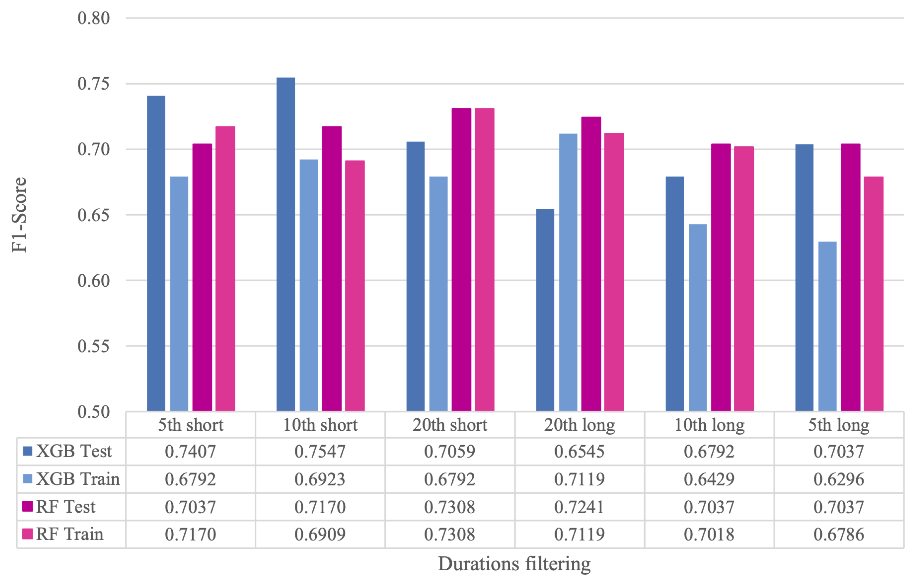
In this subsection, we have focused on analyzing the impact of audio duration on the segment reliability for AD detection. To this end, as mentioned in Section 4.3, we have proposed two different strategies. In the first one, after training the models on all the segments belonging to the training dataset, we have evaluated their performance on test sets where a specific quantile (5th, 10th, and 20th) of both the shortest and the longest audios have been discarded. In the second one, we have trained the models with the training data where certain quantiles of short and long audios have been filtered out, and subsequently evaluated their performance on the test set with the same discarded quantiles of segments.

The resulting number of audio segments in the training and test sets for all the considered quantiles after the filtering process is shown in

Table 2. Composition of the training and test subsets after the removal of the audio segments according to their duration (sec.), along with the minimum (Min.) and maximum (Max.) segment length and the percentage of segments used in the experiments.

Set	Filtering	No. of Segments	Min.	Max.	Used %
TRAIN	None	2834	0.19	10.00	100
	5th short	2653	0.32	10.00	93.61
	10th short	2546	0.34	10.00	89.84
	20th short	2260	0.45	10.00	79.75
	20th long	2267	0.19	1.76	79.99
	10th long	2550	0.19	2.35	89.98
	5th long	2692	0.19	3.00	94.99
TEST	None	1243	0.19	7.61	100
	5th short	1172	0.33	7.61	94.29
	10th short	1117	0.34	7.61	89.86
	20th short	989	0.44	7.61	79.57
	20th long	995	0.19	1.91	80.05
	10th long	1118	0.19	2.54	89.94
	5th long	1180	0.19	3.26	94.93

. Results in terms of F1-Score are contained in Figure 2, denoted as XGB Test and RF test for the XGB and RF models, respectively, and the first strategy. For the second approach, the corresponding results are named as XGB Train and RF Train for the XGB and RF models, respectively.

As can be observed, both XGBoost and RF show significant improvements when short segments are filtered out in the test set, compared to the case where no segments are eliminated. In particular, the best result for XGBoost is achieved when 10th quantile of the shortest segments are removed from the test set, while, for RF, the highest F1-Score is obtained when the 20th quantile of the shortest segments is filtered out. As for the comparison between the two strategies, whereas RF achieves similar performance, in XGBoost, the F1-Score degrades significantly when segments are removed from both the training and test sets. The exception is the case of the elimination of the 20th quantile of the longest segments. However, this configuration is discarded due to its low specificity. A plausible explanation for the XGBoost behavior is that this model is more sensitive than RF to a reduced amount of training data when the dimensionality of the input features is high.

Despite the good performance of RF, XGBoost is chosen as the reference model in the following stages of this work, as it yields the best results.

5.3. Feature Selection

In this subsection, the previously described MI and SHAP metrics have been applied as criteria for identifying and retaining the most relevant features for AD detection. For the selection experiments, the filters corresponding to the 10th and 20th quantiles of the shortest audios have been considered, given that, as observed in Section 5.2, these configurations show a compromise between performance and data reduction.

Figure 3 and Figure 4 contain, respectively, the MI and SHAP values of each feature normalized by their respective maximum value. Based on these importance values, different numbers of features (in particular, 19, 22, 25, 28, 32, 36, and 63) have been established to select subsets of them. Interestingly, these subsets exhibit significant differences. Analyzing more in depth the particular case of retaining 32 features, it can be seen that only 15 of them are the same in both cases. 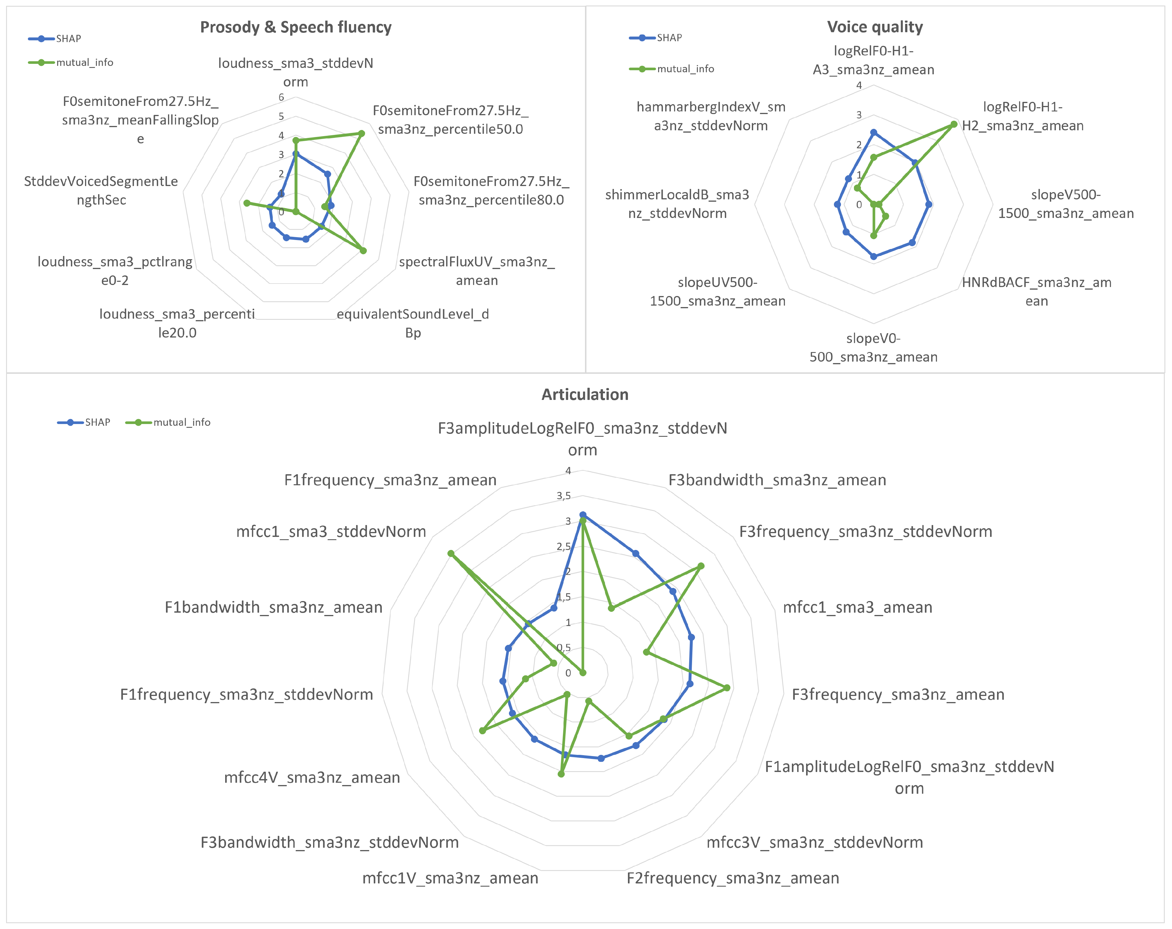Figure 5 shows the comparison between the MI and SHAP metrics for the top-32 features selected by SHAP divided into four different categories: prosody and speech fluency (in the same graph), voice quality, and articulation. As can be observed, some features with high SHAP values present low MI ones. This is the case of the voice quality parameter, representing the mean of the spectral slope in the band from 500 to 1500 Hz (slopeV500-1500_sma3nz_amean), that is ranked 12th according to SHAP, but whose MI is close to zero and is in the 56th position according to this metric (see Figure 3 and Figure 4). Another example is the articulation-related feature that measures the normalized standard deviation of the third formant bandwidth (F3bandwidth_sma3nz_stddevNorm), which occupies the 18th position in the SHAP ranking, but only the 53rd position according to MI (see Figure 3 and Figure 4).

Figure 6 shows the F1-Scores achieved by the XGBoost model with the different subsets of features determined by MI. As can be seen, the established baseline, which consists of using the complete set of features, is not exceeded. The only exception is the particular case where the 20th quantile of the shortest audios is removed during training and test, and the 28 least relevant features are discarded. This poor performance may be explained by the fact that Mutual Information measures the overall dependence of each individual feature on the target variable, but does not capture the complex interactions between input variables that are key in detecting subtle patterns, as in the case of Alzheimer’s Disease. Therefore, by eliminating features of lesser importance according to this criterion, the model loses information that could be relevant as a whole, which limits its generalizability.

Figure 7 contains the F1-Scores achieved by the XGBoost-based system with the different subsets of features selected by SHAP values. As can be seen, by removing either the 10th or 20th quantiles of the short audios only in the test set, none of the results outperform the baseline model trained with all features. However, when models are trained and evaluated excluding the shortest audio segments, certain feature selection configurations demonstrate improvements over the baseline. This difference in performance is especially notorious when filtering 10th quantile of the short audios and retaining the most relevant 22 or 32 features. This fact shows that SHAP is able to focus on the combination of features that are more informative for the AD task. In addition, utilizing lower-dimensionality inputs alleviates the data requirements necessary for effective model training, thereby taking advantage of the benefits of the segment filtering process.

As for the comparison between the MI- and SHAP-based feature selection, the results indicate a clear advantage for the SHAP-driven approach. Specifically, the highest F1-Score of $0.7692$, achieved using the top-32 features selected via SHAP under the condition of excluding the 10th quantiles of short audio samples during training and testing, significantly outperforms all feature subsets derived through MI. This performance gain can be attributed to the fact that, in contrast to MI, SHAP takes into account the interactions between features, providing a more compact and informative representation of the data.

5.4. Interpretability

For providing an interpretation of the best XGBoost model built during the previous experimental steps, we have computed the SHAP values over the samples of the training set. The resulting SHAP summary showing the 10 highest SHAP values for our task is depicted in Figure 8. Each SHAP value shows the influence of a feature on a prediction: positive values indicate that the feature pushes the prediction towards a positive class (in our case, the AD class), while negative values push it towards the negative class (in our case, the non-AD class). Therefore, those features with higher SHAP values, positive or negative, are considered more differentiating, as their specific value for a particular instance significantly influences the prediction of the model. Thus, in turn, in our specific case, as shown in Figure 8, if one example in our data has a low value in the standard deviation of the amplitude of the third formant, the model will tend to predict it as AD, since it has a high positive SHAP value. On the other hand, if the loudness standard deviation value is low, the model tends to assign it as non-AD, since it has a high negative SHAP value.

To facilitate the interpretation of the model using SHAP, it is essential to consider the distinctive speech characteristics exhibited by individuals with Alzheimer’s disease, which arise from the neurological and cognitive impairments induced by the condition. These characteristics are [35,36,37] (1) altered prosodic features, such as pitch variability, which leads to a more monotonous voice, and speech intensity (loudness), which produces a weaker voice; (2) distortions in voice quality, such as increased breathiness, hoarseness, and creakiness; (3) reduced articulation precision, which causes a decline in the clarity of speech sounds and, thus, in the overall intelligibility; and (4) slower speech rate and increased pauses and hesitations, which disrupt the natural speech fluency.

Therefore, AD produces changes in different aspects of speech: prosody, vocal quality, articulation, and verbal fluency and rhythm. As can be observed in Figure 8, the features that contribute more to the decisions made by the XGBoost model also embrace these different speech dimensions and are related to the previously mentioned speech alterations are as follows:

• F0semitonefrom27.5Hz_sma3nz_percentile50.0 and *_percentile80.0 are, respectively, the 50th and 80th percentile of the fundamental frequency. These prosodic parameters are related to the degree of variability of the pitch (intonation), which could suffer alterations in AD patients in comparison to healthy subjects;
• loudness_sma3_stddevNorm is the normalized standard deviation by the arithmetic mean of the loudness and is related to the variation in the speech intensity. The AD speech might suffer strong changes in intensity due to the increase in the number of pauses and low control of the speech volume;
• logRelF0-H1-H2_sma3nz_amean and logRelF0-H1-A3_sma3nz_amean are, respectively, the mean of the ratio of energies of the first (H1) and the second (H2) harmonics and the mean of the ration of energy of H1 to the energy of the highest harmonic in the range of frequencies of the third formant (A3). These are quality voice parameters that reflect breathy and creaky voices [37], commonly present in AD subjects;
• F3amplitudeLogRelF0_sma3_stddevNorm, F3frequency _sma3nz_amean, *_stddevNorm, and F3bandwidth_sma3nz_amean, are, respectively, the normalized standard deviation of the amplitude of the third formant (F3), the mean and normalized standard deviation of its frequency, and the mean of its bandwidth. F3 mainly correlates to lip-rounding vowels, such as $\setminus u\setminus$. The production of these types of sounds involves the activation of two distinct articulatory muscle constrictions. Due to the complexity of coordinating these muscle movements, F3 suffers alterations when muscle control is impaired, as may occur in individuals with AD [38];
• mfcc1_sma3_amean is the average of the first MFCC. It can be loosely linked to speech articulation as it corresponds to lower formants in the vocal tract. AD speech could present alterations in this parameter due to an imprecise articulation [36].

6. Discussion

Analyzing the results described in Section 5, it can be highlighted that the XGBoost model has been shown to be the most effective in detecting AD through speech signals, compared to the other ML techniques evaluated. This initial system has been subsequently refined by means of the selection of the speech segments and features more relevant to the task. The most outstanding results of the XGBoost model are summarized in

Table 3. Results achieved by the best-performing configurations of the XGBoost model in comparison to other baseline systems.

Configuration	Acc.	F1-Score	Spec.	Sens.	CM
Challenge Baseline [18]	0.6250	0.6700	-	0.7500	-
BoAW [19]	0.6250	0.6250	-	-	-
SiameseNet [19]	0.7080	0.7080	-	-	-
VGGish [22]	0.7292	0.6977	-	0.6250	-
XGBoost Baseline	0.6667	0.7037	0.5417	0.7917	13 11 5 19
Test: 10 short	0.7292	0.7547	0.6250	0.8333	15 9 4 20
Train: 10 short & 32 features	0.7500	0.7692	0.6667	0.8333	16 8 4 20

. For comparison purposes, Table 3 also presents the results achieved on the same dataset by other systems that rely solely on the acoustic modality, as is our case.

First of all, it can be observed that XGBoost (XGBoost Baseline) surpasses the baseline acoustic model proposed in the ADReSS Challenge (Challenge Baseline) [18], which consists of an Linear Discriminant Analysis classifier using the ComParE feature set from the openSMILE toolkit. Also, our best XGBoost model (Train: 10 short & 32 features) outperforms the remaining baseline systems: a BoAW model built from openSmile descriptors and an SVM as classifier [19], a Siamese network trained using a constrastive loss function [19], and a system based on embeddings extracted from the audio pre-trained model VGGish [22]. Secondly, the removal of the 10th quantile of short segments in the test (Test: 10 short) produces a relative improvement of $7.24\%$ in F1-Score, $15.38\%$ in specificity, and $5.25\%$ in sensitivity with respect to XGBoost Baseline. Thirdly, the selection of the 32 most relevant features using SHAP values in combination with the discarding of the 10th quantile of short segments in training and test (Train: 10 short & 32 features) further optimizes the model’s performance. In this case, the relative improvements regarding XGBoost Baseline are $9.31\%$, $23.08\%$, and $5.25\%$ for, respectively, F1-Score, specificity, and sensitivity.

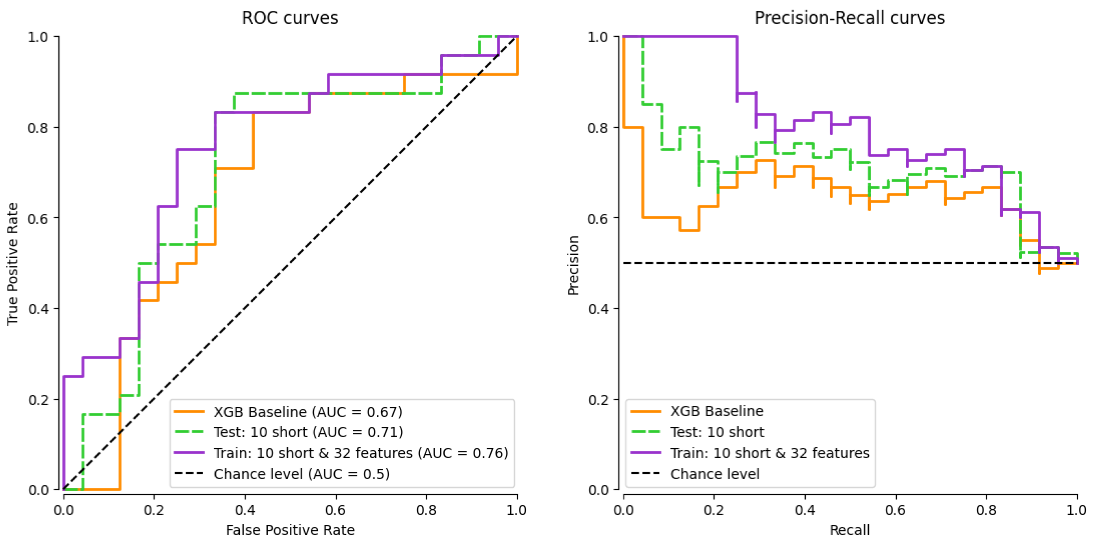
For completeness, Figure 9 depicts the Receiver Operating Characteristic (ROC) curve along the corresponding Area Under the Curve (AUC) values (left), and the Precision–Recall (PR) curves (right) of the XGBoost model with the best configurations. The good performance of the proposed segment and feature selection techniques can be explained by the nature of the data and the model’s decisions during the learning process. By removing the shortest segments, speech segments containing less relevant information or having more noise, such as interjections or single syllables, are discarded. This improves the quality of the dataset and, therefore, the reliability of the model. Nonetheless, it is important to recognize the inherent trade-off between excluding noise and retaining diagnostically relevant short utterances. In addition, the SHAP-based feature selection enables the choice of the input variables that have the greatest influence on predictions, allowing the model to focus its learning on the most differentiating aspects of the input. As can be drawn from the results in Table 3, the combination of both techniques improves model generalization and consequently increases all the considered metrics. Moreover, the simplification of the model by reducing the number of features has a profound impact on interpretability. A model with fewer features is inherently easier to analyze and understand, as this reduces the complexity involved in deciphering how different variables influence predictions.

An example of the interpretability power of SHAP is depicted in Figure 10, which shows the contributions (SHAP values) of the features to the prediction of a specific test sample, which has been classified as presenting AD with a model output $f\left(x\right)=0.555$. This output is derived from the best XGBoost model. In this case, the base value (expected output $E\left[f\right(X\left)\right]$) starts at approximately $-0.154$, which is the mean model prediction across all samples in the training data. From this value, it can be seen that the contribution of some features pushes the model’s prediction towards (in red) or away from (in blue) the final output of $f\left(x\right)=0.555$. The features that stand out in this prediction are mainly related to the speech articulation, except for the logRelF0-H1-H2_sma3nz_amean, which is a voice quality parameter, and StddevVoicedSegmentLengthSec, which corresponds to the regularity of the duration of the voiced regions (speech fluency).

Beyond standard performance metrics like F1-Score, it is important to highlight that the best-performing XGBoost model (Train: 10 short & 32 features) also demonstrates a satisfactory clinical utility, as shown in

Table 4. CUI values for the best-performing configurations of the XGBoost model.

Configuration	F1-Score	CUI+	CUI-	Total CUI
XGBoost Baseline	0.7037	0.5014	0.3912	0.4463
Test: 10 short	0.7547	0.5747	0.4934	0.5341
Train: 10 short & 32 features	0.7692	0.5952	0.5333	0.5643

. In particular, this system achieves the highest total CUI of $0.5643$, indicating a balanced performance in both positive and negative utility. This outcome, along with the model’s overall accuracy, suggests that, although there is room for improvement, the XGBoost model is not only effective in detecting Alzheimer’s from speech data but also exhibits satisfactory practical utility, making it a potentially valuable tool for clinicians in real-world diagnostic settings.

Finally, in terms of computational cost, the best model shows a significant reduction in both the number of datapoints and the number of features without compromising its performance. By eliminating short audio segments, a noticeable decrease in the size of the training and test dataset is achieved. Combined with the reduction to the 32 most relevant features according to the SHAP values, the model experiences a decrease of close to 70% in the smallest configuration compared to the base case, as is shown in

Table 5. Amount of training and test data used in the best configurations of the XGBoost model.

Configuration	Data Train	Data Test	% Used
XGBoost Baseline	2834 segments × 88 features	1243 segments × 88 features	100
Test: 10 short	2834 segments × 88 features	1117 segments × 88 features	96.91
Train: 10 short & 32 features	2546 segments × 32 features	1117 segments × 32 features	32.67

. This reduction not only decreases training time and memory requirements, but also optimizes the use of computational resources, which is crucial for applications in time- and processing-constrained environments. Despite the reduction in the amount of data and number of features, the results obtained remain competitive and even improve, demonstrating the effectiveness of the filtering methods applied to maintain a balance between performance and efficiency.

Limitations

Despite the promising outcomes of this study, several limitations must be acknowledged. First, although the best XGBoost model achieved a strong F1-score, this metric still indicates room for improvement in either sensitivity or precision, both of which are particularly critical in clinical applications where diagnostic accuracy has significant implications.

Second, the generalizability of our approach may be constrained by the use of a single dataset, limiting the ability to draw conclusions applicable to broader clinical contexts.

Third, while SHAP values have been employed to enhance model interpretability, their practical utility in real-world deployment requires clinicians’ understanding and trust in AI-based systems. This highlights the necessity of clinician training and user-centered design as part of the implementation process.

Lastly, although our study has been conducted on a dataset balanced for age and gender, we have not explicitly examined potential biases in data collection or acoustic feature extraction. On the one hand, a limited representation of diverse populations may lead to reduced model performance for underrepresented groups, potentially worsening healthcare disparities. On the other hand, variations in speech patterns linked to age, gender, or socio-cultural background and the risk of acoustic features encoding demographic information could introduce bias and confounding effects. These issues highlight the importance of using fairness-aware evaluation metrics and ensuring demographic diversity in datasets to promote equitable and accurate AI applications in clinical contexts.

7. Conclusions

In this work, we have developed an XGBoost-based system for Alzheimer’s Disease detection from spontaneous speech using exclusively acoustic cues. The results obtained show that the system is not only capable of delivering accurate predictions but also offers a balance between computational efficiency and interpretability, achieving the objectives set at the beginning of this research work. A key aspect of this approach has been the use of SHAP values, which have proven to be a highly promising tool, both for feature selection and for gaining deeper insights into the decision-making process of the models. The ability to identify the most relevant features and explain their impact on individual predictions adds significant value, particularly in clinical applications where transparency is essential.

Future work will involve validating our approach on diverse datasets that better represent a broad range of populations, with particular emphasis on analyzing potential biases in both the datasets and the speech feature extraction process. Another research line that we plan to follow is the incorporation of new ML paradigms, such as multi-task and multi-view learning, for improving the performance of the models in scarce training data conditions. In addition, other state-of-the-art XAI methods, such as Local Interpretable Model-Agnostic Explanations (LIME) [39] and Concept Bottleneck Models (CBM) [40], will be explored for enhancing the interpretability of the developed systems.