Abstract
In rolling bearing fault diagnosis, faint fault features are often obscured by ambient noise, limiting the feature extraction capabilities of traditional methods. To address this problem, a time and frequency domain blind deconvolution method based on the generalized norm (G-Lp/Lq-TF) is proposed. Through an analysis of the generalized norm’s properties, two monotonic yet opposing sparsity-related value intervals are identified and applied separately in the time and frequency domains. The optimal selection range for p and q values is then determined. A hybrid optimization criterion is designed to enforce mutual constraints between the two intervals, ensuring an optimal solution. A convolutional neural network is utilized to serve as the blind deconvolution filter, with backpropagation-based automatic differentiation used for gradient-based optimization of filter coefficients. This approach provides adequate decision-making guidance for selecting p and q values, which was lacking in previous studies on the sparsity of the generalized norm. It also mitigates noise-spike sensitivity and frequency component loss when applied independently in either domain. Validation using simulated signals and three real-world bearing fault datasets confirms that the proposed method outperforms existing methods in both fault feature extraction and stability.
1. Introduction
Rolling bearings have been widely utilized across various industrial sectors, including manufacturing, energy transportation, and petrochemical industries. Due to their frequent operation under heavy loads, high speeds, or other harsh conditions, they are highly susceptible to damage [1]. Faulty bearings can lead to severe consequences, such as unplanned downtime and even potential threats to personnel safety. Hence, real-time condition monitoring and early detection of bearing faults are critically important. Accurately assessing bearing health and identifying fault types remain significant challenges. Due to the structural characteristics of rotating machinery, acceleration sensors are typically mounted externally. As a result, the acquired signals are often affected by noise and the system’s structural dynamics, making it difficult to directly observe bearing fault features [2,3,4]. Therefore, the effective extraction of fault-related information from complex signals constitutes a critical step in fault diagnosis.
On this basis, scholars have designed and proposed a range of effective methods for fault feature extraction. Sparse representation and sparse index-based approaches include variational mode decomposition (VMD) [5,6], wavelet transform (WT) [7,8], and blind deconvolution methods (BDMs) [1,9]. Adaptive signal decomposition-based methods comprise local mean decomposition (LMD) [10,11] and empirical mode decomposition (EMD) [12,13], while other techniques include spectral kurtosis (SK) [14,15] and singular value decomposition (SVD) [16,17]. Among them, BDM reconstructs fault-related impulses by designing filters to suppress the impact of transmission paths on the signal. This method adaptively adjusts the coefficients based on optimization criteria to derive the optimal filter, free from constraints imposed by bandwidth and center frequency [18]. Given its effectiveness in overcoming the challenges of eliminating transmission path effects in fault feature extraction, BDM has garnered extensive research and application, gradually emerging as one of the primary methods in fault diagnosis.
Classical BDMs primarily include minimum entropy deconvolution (MED) [19,20]. These classical algorithms primarily optimize time-domain signals. Originally introduced in seismology [21], MED utilizes kurtosis as an optimization criterion to determine the optimal filter coefficients, thereby extracting impulsive components from the signal. However, when external shocks or interference exceed the impact of the actual fault, this method may misidentify noise impulses as fault-related features. To address this problem, researchers incorporated the concept of fault signal periodicity into the classical MED framework, leading to the development of the maximum correlated kurtosis (MCKD) method [22]. Although it improves the extraction of periodic fault features, its strong dependence on prior feature input presents a significant limitation. Subsequent algorithms, such as sparse harmonic-to-noise ratio deconvolution (SHMD) [23,24], second-order cyclostationary blind deconvolution (CYCBD) [25], and optimal minimum entropy deconvolution (OMED) [19], have been proposed to mitigate this dependency. However, none have fundamentally overcome the challenge of reliance on prior knowledge.
Furthermore, BDM also includes algorithms based on generalized norms. Compared to traditional BDM methods, these algorithms offer greater flexibility, enhanced robustness, and superior performance in sparse signal processing. Due to their ability to address challenges that conventional approaches struggle with they have garnered attention from researchers. Jia et al. conducted a geometric analysis of the generalized norm and integrated its sparsity properties with blind deconvolution, proposing a blind deconvolution method based on sparse feature extraction [26]. The SF-SLSN method leverages the generalized norm to restore fault features in the time domain, effectively capturing transient impulses in the signal [27]. However, the extracted signal contains not only fault-induced transient impulses but also noise-induced transients, which may be mistakenly identified and extracted. To address this limitation, the Mini-blp-lplq method employs the generalized norm to reconstruct sparse envelopes in the envelope spectrum, thereby enhancing fault feature extraction while effectively mitigating noise misidentification [28]. Despite achieving promising results, relying solely on the frequency domain for feature extraction poses challenges, such as insensitivity to impulsive components and the risk of frequency loss.
In recent years, deep learning has been widely adopted in fault diagnosis due to its superior capability in handling complex information and its intelligent adaptability during operation. Cao et al. [29] employed deep learning to analyze magnetic field data for locating and quantitatively assessing high-resistance connection faults in motors, achieving favorable results in both accuracy and fault identification. Guo et al. [30] developed a dual-channel network based on convolutional block attention modules and a nonlinear Wiener process with random effects to construct health indicators and predict the remaining useful life of bearings, yielding high prediction accuracy. Wang et al. [31] integrated fractional diversity entropy into a classifier-guided diffusion model, enhancing the quality of synthetic samples and improving diagnostic accuracy for bearings, gearboxes, and rotors. Despite important progress, deep learning-based fault diagnosis still faces the challenge of accuracy being heavily dependent on model complexity.
In summary, the generalized norm effectively captures sparse components and transient impulses when applied in the time domain. However, it may misinterpret noise-induced spikes as signal impulses, leading to erroneous feature extraction, while also overlooking harmonic frequency components within the signal. In contrast, its application in the frequency domain provides a more global perspective on signal characteristics but lacks sensitivity to transient impulses, which can result in frequency component loss and diminished sparsity compared to the time domain. To overcome these limitations, the generalized norm is applied in both the time and frequency domains, utilizing their complementary advantages. First, an analysis of the generalized norm reveals two distinct intervals with opposing characteristics. Based on the properties of these intervals and the parameter , the impact on sparse feature extraction is systematically assessed. The most suitable ranges in both the time and frequency domains were determined. Building on this insight, a hybrid time and frequency optimization criterion is proposed. This criterion exploits the opposing and monotonic sparsity properties of the generalized norm across different intervals, ensuring that the extraction process is constrained by both characteristics. This approach enables a more comprehensive capture of signal features while mitigating overfitting during optimization. It not only augments algorithmic performance but also significantly enhances overall stability. To address this, only a two-layer convolutional neural network was utilized as the filter in the blind deconvolution framework, thereby reducing model complexity while enabling the attainment of optimal solutions through a hybrid optimization criterion.
Main contributions of this paper:
- (1)
- To overcome the limitations of applying the generalized norm exclusively in either the time or frequency domain, we propose a time and frequency domain blind deconvolution algorithm based on the generalized norm. This algorithm integrates optimization criteria from both domains and employs a backward automatic differentiation algorithm to compute gradients for optimizing the blind deconvolution filter.
- (2)
- To determine the optimal selection of and , we derived and analyzed the characteristics of the generalized norm in measuring signal sparsity. Additionally, a reference approach for selecting the value in both time and frequency domains is proposed.
The remainder of this paper is structured as follows: Section 2 introduces the time and frequency domain blind deconvolution algorithm based on the generalized norm. It offers an in-depth exploration of the fundamental principles of blind deconvolution and its implementation process, and discusses the properties of the generalized norm along with the selection of optimization criteria. Section 3 presents the design of simulated fault signals and evaluates the proposed method’s noise resistance and fault feature extraction capability using these signals. The results demonstrate that our method outperforms existing methods. Section 4 validates the proposed approach using the CWRU bearing fault dataset, along with the XJTU-SY and IMS full-lifecycle bearing datasets. The experiments further confirm the method’s effectiveness in fault feature extraction and full-lifecycle bearing condition monitoring.
2. Methodology
2.1. Blind Deconvolution Theory
During vibration signal acquisition, the path through which the fault source signal reaches the sensor is typically considered a convolutional process. Blind deconvolution refers to the process of reversing convolution. By simplifying the signal transmission path into a single function, Equation (1) is obtained.
where denote the measured signal, represent the raw signal, denotes the unavoidable internal noise of the measurement system, and corresponds to the harmonic signal generated by rotational meshing [32,33]. The transfer functions are represented by , and , with denoting the convolution operation.
Since the transfer functions are unknown, the technique of recovering the raw signal from the measured signal is referred to as the blind deconvolution process, as expressed in Equation (2).
where represents the filter, and denotes the recovered signal.
The core principle of blind deconvolution is to design an inverse filter that effectively suppresses noise, harmonics, and other interferences, allowing the filtered measured signal to be restored as accurately as possible to its original state. Figure 1 illustrates the process of signal convolution, where the original bearing fault signal transforms into the measured signal, as well as the inverse deconvolution process, which restores the measured signal back to its original form.
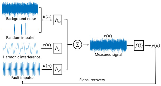
Figure 1.
A schematic diagram of the deconvolution of bearing fault signals.
2.2. Time and Frequency Domain Blind Deconvolution Based on Generalized Norm
The proposed G-Lp/Lq-TF is an algorithm that independently processes the time and frequency domains by leveraging the distinct properties of the generalized norm over different value intervals. This algorithm independently processes the time and frequency domains by leveraging the distinctive properties of the generalized norm across different value intervals. Additionally, a hybrid optimization criterion is designed to guide the algorithm’s optimization process. In the time domain, the method employs the interval , while in the frequency domain, it utilizes the interval . Theoretically, this approach mitigates the issue of noise spikes being misclassified as signal impulses when solely relying on the time domain, in addition to the problems of frequency component loss and insufficient sparsity when using only the frequency domain. The theoretical analysis is as follows: Given the opposite and monotonic sparsity characteristics of the generalized norm in these two intervals, the algorithm is designed with a hybrid optimization criterion that enables mutual constraints between the time and frequency domain optimization criteria, thereby reducing the risk of overfitting in either domain. Consequently, the algorithm achieves both high performance and strong stability. Figure 2 illustrates the framework of the time and frequency domain blind deconvolution algorithm based on the generalized norm, depicting the process of a single iteration.

Figure 2.
Time and frequency domain blind deconvolution framework using generalized norm.
Firstly, a dual-layer convolution structure is adopted, with each layer constructing a deconvolution filter, thereby effectively utilizing two deconvolution filters. To ensure that the input signal maintains its original size after passing through both deconvolution filters, zero-padding is applied to both ends of the signal before convolution filtering. Secondly, the filtered signal in the time domain remains unchanged, whereas, in the frequency domain, the signal undergoes Hilbert transform, followed by envelope extraction and fast Fourier transform (FFT), ultimately yielding the envelope spectrum signal. For the time domain signal, the generalized norm is applied within the interval, while for the frequency domain signal, the norm is utilized in the interval. Consequently, two optimization metrics, and , are obtained and unified onto the same scale using Equation (3) before summation, facilitating the minimization of the loss function via deep learning optimizers.
The obtained objective function is used for backpropagation automatic differentiation to compute the gradient of each filter. Compared with other differentiation algorithms, backpropagation automatic differentiation offers higher precision and faster computation speed. This algorithm is driven by the chain rule, as expressed in Equation (4).
The input signal undergoes the following filtering procedure.
where and are deconvolution filters of length L, with L being a predefined value. represents the filtered signal and is the input signal.
Assuming , the gradient of in this algorithm can be computed using the chain rule:
where is computed based on the minimization criterion.
Similarly, the gradient of is calculated as follows:
Once the gradients of the filters are computed through backpropagation automatic differentiation, use Adam to update the filter coefficients and complete one iteration. After multiple rounds of iterations, the objective function gradually converges, ultimately yielding the filtered signal from the time and frequency domain blind deconvolution algorithm using the generalized norm.
2.3. Design of the Blind Deconvolution Filter
2.3.1. Derivation of the Generalized Norm
The generalized norm was initially developed through the derivation of the L1/L2 norm. The generalized norm can be traced back to the MED obtained through Gary’s variational method, also referred to as variable norm deconvolution [34]:
where represents the signal and denotes the signal length. Subsequently, a -mean formulation similar to Gary’s variable norm was proposed [35], defined as follows:
The optimization strategy of the generalized norm varies depending on the ratio . To unify sparsity indices within a single framework, the term is introduced into the formulation, yielding the following generalized norm:
2.3.2. Analysis of the Properties of the Generalized Norm
serves as an effective sparsity metric, characterized by scale invariance and enriched gradient information. These properties enhance its robustness in maintaining input signal scale during computation and streamline the optimization process. The relationship between and sparsity under varying values is illustrated in Figure 3. The input parameter is drawn from a Bernoulli distribution, where the probability of a coefficient being zero is denoted as p0 (ranging from 0 to 1). An elevated p0 value implies that most extracted coefficients are predominantly zero, signifying increased sparsity. By analyzing the relationship curves between and sparsity under different values.
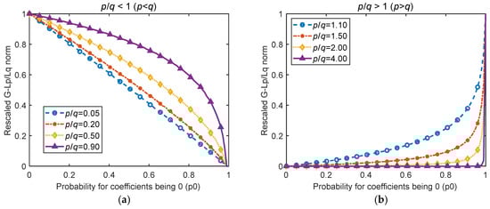
Figure 3.
The relationship between the generalized norm and probability p0. (a) to sparsity under , (b) to sparsity under .
- (1)
- When , the function curve is monotonically decreasing, implying that minimizing enhances sparsity. Conversely, when , the function curve is monotonically increasing, suggesting that maximizing also improves sparsity. Theoretically, adjusting the optimization strategy based on different values can effectively enhance sparsity.
- (2)
- In the scenario, the effect of different values on sparsity is relatively consistent. Notably, when , the relationship approximates linearity, indicating a uniform gradient descent that facilitates filter optimization. In the scenario, the impact of varying values on sparsity is noteworthy. Particularly, when , smaller changes in result in a slow increase in sparsity, which remains close to zero. When reaches 0.1, the sparsity increases sharply, which is detrimental to gradient-based optimization. Therefore, values within this range should be avoided when selecting parameters.
The generalized norm encompasses two optimization criteria, necessitating the computation of its first derivative for further analysis. The characteristics of these optimization criteria are examined as follows:
where denotes the index corresponding to the maximum absolute value of the signal .
Differentiating yields the following:
where , .
For , the following inequality holds:
Substituting Equation (13) into Equation (12) yields:
Similarly, for , the following inequality holds:
Substituting Equation (15) into Equation (12) yields:
From Equation (14), it follows that when , the generalized norm increases monotonically with the largest absolute value in signal . As shown in Figure 3, in the process of maximizing to achieve higher sparsity, the increasing value approaches the maximum absolute value of . Consequently, under , the generalized norm exhibits high sensitivity to single peaks within the signal. From Equation (16), it follows that when , the generalized norm decreases monotonically with the largest absolute value in signal . As illustrated in Figure 3, in the process of minimizing to enhance sparsity, the decreasing value also converges to the maximum absolute value of . Therefore, the norm minimization strategy within the range also exhibits sensitivity to unimodal features. In summary, the blind deconvolution method based on the generalized norm exhibits high sensitivity to single peaks across all parameter intervals. If applied indiscriminately, this method may be susceptible to noise-induced single-peak effects. To further examine the influence of and on single-peak sensitivity, the peak characteristics of the generalized norm are derived under varying values. Performing a limit analysis on in yields the following:
From Equations (17) and (18), it is observed that as p approaches positive infinity, the generalized norm increasingly emphasizes the dominant peak values within the signal. Conversely, as approaches zero, the norm remains unaffected by individual peak values. This leads to the conclusion that, compared to larger values, the generalized norm with smaller values is less influenced by individual peaks in the signal. Therefore, when selecting values, it is generally preferable to choose smaller values to mitigate peak sensitivity effects.
2.3.3. Selection of Optimization Criteria for Generalized Norm in Time and Frequency Domain
The generalized norm was applied to process an outer ring fault signal of a bearing, and the corresponding generalized L1/L2 norm values under various and , combinations are plotted in Figure 4. A smaller generalized L1/L2 value indicates enhanced sparsity in the filtered signal, reflecting more pronounced impulsive characteristics in the input data. The following observations can be drawn from Figure 4:
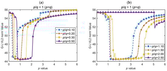
Figure 4.
Sparsity of filtered signals for different and values. (a) Relationship between and G-L1/L2 for different values when . (b) Relationship between and G-L1/L2 for different values when .
- (1)
- When , the optimal sparsity distribution remains highly consistent across different values, achieving robust sparsity. For , the sparsity distribution also exhibits consistency, but a prominent shift occurs when . Therefore, this value should be avoided when selecting a ratio.
- (2)
- Selecting an appropriate -value ensures optimal sparsity across different ratios. There exists an optimal range for , which expands as increases. Larger ratios provide greater flexibility in choosing .
- (3)
- In the range , setting yields greater sparsity and is a preferred choice. Similarly, for , setting serves as an ideal starting point for adjusting the generalized norm.
From the analysis in Figure 3, different values can yield satisfactory sparsity, making gradient optimization a key consideration when selecting . According to Equation (17), smaller values in the generalized norm are less affected by single peaks in the signal compared to larger -values. As observed in Figure 4b, -values in the range of 2 to 4 also result in favorable sparsity, indicating that the optimal -value range is broader for Figure 4b than for Figure 4a. Considering that time-domain methods are more sensitive to sharp peaks, while frequency-domain methods are less responsive to transient impacts, selecting a larger -value in the time domain than in the frequency domain enhances the performance of the generalized norm across both domains. Specifically, choosing in the time domain and in the frequency domain leverages the monotonic but opposite characteristics of the norm across these intervals. This approach forms an optimization criterion that enables mutual constraints in time and frequency domains, compensating for their respective limitations and achieving a more comprehensive signal feature extraction.
To validate the accuracy of the selected optimization criteria in the time and frequency domain, Figure 5 illustrates the filtering performance of the same signal using different combinations of optimization criteria, with red dashed lines indicating bearing fault frequencies and their harmonics. The first row of images presents results when the criterion is applied in both time and frequency domains, while the second row shows results using in both domains. The envelope spectrum in the first row reveals that the criterion tends to extract individual frequency components, whereas the spectrum in the second row indicates that the criterion is more susceptible to noise interference. Analysis of these two combinations reveals that an unconstrained optimization criterion results in overfitting, potentially causing the omission of critical fault-related components. The third and fourth rows present results obtained by applying different optimization strategies in the time and frequency domains. The third row adopts an approach opposite to the aforementioned analysis, and its envelope spectrum reveals a greater loss of fault feature components compared to using a uniform optimization criterion. The fourth row illustrates the results obtained by selecting the most appropriate optimization criteria as per the above analysis. The envelope spectrum clearly shows that fault feature components are effectively extracted, with minimal interference from shaft rotational frequencies and noise compared to the other three configurations. Experimental results demonstrate that selecting optimization criteria with in the time domain and in the frequency domain yields the most effective fault feature extraction.
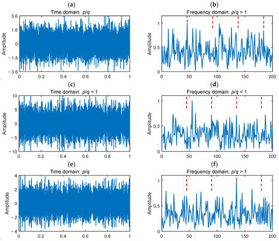
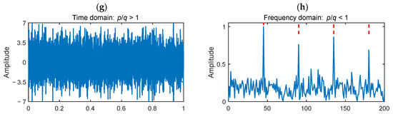
Figure 5.
Comparison of different optimization criteria combinations in time and frequency domain. (a,c,e,g): Time-domain representations of the filtered signals. (b,d,f,h): Envelope spectra of the filtered signals. The red dashed lines indicate the bearing fault frequencies and their harmonics.
3. Experiment
3.1. Experimental Setups
Based on the optimal combination of time and frequency domain optimization criteria, adopting an optimization condition with in the time domain and in the frequency domain yields superior fault feature extraction performance. As illustrated in Figure 4, when , the p-value ranges from 1 to 4; when , it ranges from 0.5 to 2, which leads to improved sparsity. The generalized norm is employed for experimental validation, with , selected in the time domain and , in the frequency domain. The selected comparison methods include MCKD [22], MED [19], Mini-blp-lplq [28], and SF-SLSN [27], with their recommended parameters applied for optimization. Our method was implemented using TensorFlow in Python 3.10. The learning rate was configured at 0.01, the filter length to 40, and the Adam optimizer was employed for 200 training iterations [36]. The hardware environment consisted of an Intel i9-12900K CPU, a 16GB × 2 of DDR5 RAM, and an NVIDIA GeForce RTX 3090 GPU.
3.2. Method Validation on Simulated Signals with High Noise
3.2.1. Mathematical Model of Rolling Bearing Vibration
A bearing vibration mathematical model [37,38] was employed to generate simulated measured signals embedded with various types of interference and noise. Simulated signals generated by the model are employed to evaluate the feature extraction capability of the signal filtering method. This mathematical model comprises four components: (i) Impulse signals simulating faults in rolling bearings. (ii) Impact signals mimicking external strikes or electromagnetic interference. (iii) Harmonic interference caused by gears, blades, shafts, or other rotating components. (iv) Gaussian white noise, modeled as follows:
In the first component, represents the amplitude modulation of the -th impact, denotes the interval between periodic impulses, and is a random variable representing the slip of the -th roller, typically 1–2% of . The explicit formulation of is as follows:
where , is the damping factor of the single-degree-of-freedom system, represents the initial phase, and is the resonant frequency of the -th impact.
In the second component, and are modeled as random variables due to their unpredictability.
In the third component, , , and are parameters of the periodic harmonic signal, where is the initial phase, is the frequency, and is the amplitude.
3.2.2. Simulation of Bearing’s Inner Race Fault Signals
In this situation, simulated signals exhibiting localized defects are generated. The characteristic frequency of the fault was configured at 45 Hz, with a signal-to-noise ratio (SNR) of −16 dB for the Gaussian white noise . The sampling frequency was configured at 20 kHz [39,40]. The specific parameters of the remaining synthetic signals are summarized in Table 1. The simulated fault impulses, random pulses, harmonic interference, Gaussian noise, and their combination are illustrated in Figure 6. Clearly, the fault impulse signals are entirely submerged in high-intensity noise.

Table 1.
Parameters of synthetic signal.
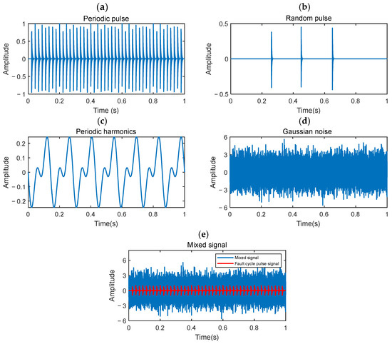
Figure 6.
Simulated signal. (a) Periodic pulse; (b) Random pulse; (c) Periodic harmonics; (d) Gaussian noise; (e) Mixed signal.
Figure 7 presents the simulation results, where red dashed lines indicate the bearing fault frequency and its harmonics. In the time-domain comparisons between the filtered and raw signals, all methods partially restored the impulse characteristics to varying degrees. The envelope spectra of G-Lp/Lq-TF, Mini-blp-lplq, and SF-SLSN clearly reveal fault-related harmonics, effectively identifying the simulated bearing fault. However, the results derived from MCKD and MED are relatively disordered, making it difficult to discern the harmonics associated with fault characteristic frequencies. Table 2 presents the kurtosis values of the signals after filtering using the respective methods. Notably, the G-Lp/Lq-TF method achieved a kurtosis value of 4.1769, surpassing both other methods and the raw signal’s kurtosis of 2.8958. This demonstrates its superior capability in extracting impulse characteristics. Compared to other approaches, this method exhibits robustness against single impulses in high-noise environments and effectively suppresses low-frequency noise, making it the most precise and effective in fault feature extraction. Overall, the proposed method demonstrates superior and more stable performance in bearing fault detection under high-noise conditions compared to existing methods.
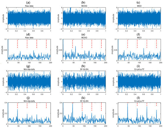
Figure 7.
Diagnosis results: (a–c,g–i) show the time-domain signals processed by different methods, while (d–j,k,l) show their corresponding envelope spectra. The red dashed lines indicate the bearing fault frequencies and their harmonics.
Table 2.
Kurtosis values of different methods on simulated signals.
3.3. Method Validation on Real Bearing Fault Signals
3.3.1. Fault Diagnosis on the CWRU Dataset
This bearing vibration dataset was provided by Case Western Reserve University (CWRU) [41]. The test platform primarily consists of several components: a motor, accelerometers a torque sensor, and a power meter. In the case of including health signals, the dataset comprises ten different fault types. This study utilizes vibration signals recorded at 12 kHz under 1 HP and 3 HP load conditions. The detailed bearing specifications are provided in Table A1 of Appendix A.
Datasets under load conditions of 1 HP and 3 HP were selected to evaluate the method’s effectiveness, with 4800 data points extracted for each operating state. Table 3 lists the kurtosis values corresponding to the filtered signals. SF-SLSN and MED achieved kurtosis values mostly higher than the raw signal, though slightly lower in certain cases, yielding generally favorable results. MCKD showed inconsistent performance, with some values exceeding and others falling below the raw signal, highlighting its instability and dependence on prior knowledge. Mini-blp-lplq exhibited only minor improvements in time-domain kurtosis, with most values slightly below those of the raw signal. G-Lp/Lq-TF exhibits the highest kurtosis across all three fault types, demonstrating a notable improvement compared to the kurtosis of the raw signals. Notably, the kurtosis values of most fault-filtered signals are elevated to nearly three times those of the raw signals.
Table 3.
Kurtosis values of different methods on the CWRU-1HP and CWRU-3HP datasets.
As depicted in Figure 8, the time-domain signal and envelope spectrum corresponding to the inner race fault under the 3HP operating condition are depicted, with the red dashed lines marking the characteristic fault frequency and its harmonics. The formulas for calculating bearing fault frequencies are presented in Appendix B. In the raw signal, fault-induced impulses are barely distinguishable in the time domain due to the extended transmission path to the sensor. In the envelope spectrum, only the fundamental frequency and its first harmonic are observable, while other harmonics remain nearly imperceptible. MCKD failed to extract any fault frequencies, further confirming its limitations due to reliance on prior knowledge. While MED performed slightly better than the raw signal, its extracted harmonic components remained unclear. Mini-blp-lplq and SF-SLSN also failed to extract additional fault harmonics. In contrast, G-Lp/Lq-TF significantly enhanced fault-related harmonic components, effectively reinforcing fault signal features and mitigating transmission path effects. These results confirm the method’s ability to enhance fault characteristics and its superior stability across different scenarios.
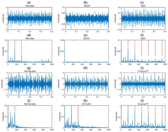
Figure 8.
Diagnosis results: (a–c,g–i) show the time-domain signals processed by different methods, while (d–j,k,l) show their corresponding envelope spectra. The red dashed lines indicate the bearing fault frequencies and their harmonics.
3.3.2. Fault Diagnosis on the XJTU-SY Dataset
Experiments were conducted using the XJTU-SY rolling bearing accelerated degradation dataset, provided by Xi’an Jiaotong University (XJTU) and Zhejiang Changxing Shengyang Technology Co., Shaoxing, China [42]. The dataset comprises complete operational failure data of 15 rolling bearings under three distinct operating conditions. In this study, the Bearing3_3 dataset was utilized, and recorded at a motor speed of 2400 rpm, a radial load of 10 kN, and a total operational duration of 6 h and 11 min, with an inner race failure occurring at 340 min. The detailed bearing specifications are provided in Table A2 of Appendix A.
Leveraging the property of increased kurtosis in fault signals, the measured signals were processed using various methods, and their kurtosis values were computed to identify fault occurrence based on kurtosis variation. Figure 9 presents the kurtosis variation over 371 min of bearing operation for the proposed and comparative methods. By identifying the initial significant kurtosis change in each method, the stability of each approach on healthy signals and its sensitivity to faults were evaluated. Table 4 lists the times at which different methods detected abrupt kurtosis changes. MCKD, Mini-blp-lplq, and SF-SLSN exhibited large fluctuations in kurtosis when processing healthy vibration signals. In particular, MCKD and Mini-blp-lplq prematurely detected abnormal kurtosis values of 6.8432 and 5.8838 at 143 min and 21 min, respectively, leading to misidentification of the fault state. SF-SLSN yielded an anomalous kurtosis of 7.1373, significantly exceeding the raw signal, but it suffered from detection delay, identifying the fault only at 344 min. Both G-Lp/Lq-TF and MED successfully detected the fault at 340 min. However, G-Lp/Lq-TF achieved a kurtosis value of 7.2573, markedly higher than both the raw signal (3.3750) and MED (5.0574). While MED exhibited two notable transient fluctuations during healthy signal processing, G-Lp/Lq-TF demonstrated greater stability and superior sparse feature extraction.
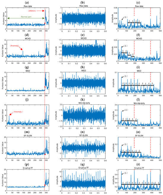
Figure 9.
Diagnosis results: (a,d,g,j,m,p) show the kurtosis variation across the full lifecycle for each method. (b,e,h,k,n,q) show the time-domain signals at 340 min. (c,f,i,l,o,r) show the envelope spectra at 340 min. The red dots in the kurtosis variation plot indicate the kurtosis values at the moment of fault occurrence, while the red dashed line marks the reference line at 340 min. In the envelope spectrum, the red dashed lines represent the bearing fault frequency and its harmonics.
Table 4.
Earliest kurtosis mutation times and corresponding kurtosis values in the XJTU-SY dataset.
The time-domain waveform and corresponding envelope spectrum at the 340-min mark were also plotted, with red dashed lines marking the bearing fault frequency and its harmonics, as shown in Figure 9. In the raw signal, neither the impulse signals nor the fault and spindle rotational frequencies are clearly visible in the envelope spectrum. MCKD, Mini-blp-lplq, and SF-SLSN primarily enhanced the spindle rotational frequency components while failing to reveal the fault characteristic frequencies, highlighting the limitations of prior knowledge-based methods and approaches that process only in the time or frequency domain. In contrast, G-Lp/Lq-TF and MED effectively extracted fault characteristic frequencies and enhanced fault signal features. Notably, G-Lp/Lq-TF demonstrated superior performance in distinguishing spindle rotational frequency from fault characteristic frequency, emphasizing fault-related components more prominently.
To evaluate the performance of each method using the envelope spectrum, the Hilbert envelope spectrum fault feature ratio [43] was introduced.
where denotes the total amplitude of the envelope spectrum, represents the envelope spectrum amplitude at the corresponding frequency, and is the characteristic fault frequency of the bearing.
A higher Hilbert envelope spectrum fault characteristic ratio indicates a more effective fault feature extraction method. As shown in Table 5, the characteristic ratio obtained by MCKD is lower than that of the raw data, suggesting limited fault feature enhancement. In contrast, MED, Mini-blp-lplq, SF-SLSN, and G-Lp/Lq-TF yield higher ratios than the raw data. Among them, G-Lp/Lq-TF achieves the highest ratio at 3.34%, demonstrating the most effective fault feature extraction in the envelope spectrum. Experimental results indicate that G-Lp/Lq-TF exhibits remarkable stability when processing healthy vibration signals. Compared to alternative methods, it exhibits enhanced sensitivity to fault signals and demonstrates superior diagnostic performance for early bearing failures.
Table 5.
Hilbert envelope spectrum fault feature ratio of XJTU-SY data.
3.3.3. Fault Diagnosis on the IMS Dataset
This section presents tests conducted using the full-lifecycle rolling bearing dataset provided by the Center for Intelligent Maintenance Systems (IMS) at the University of Cincinnati [44]. This dataset comprises three subsets, each containing experimental data from four bearings. The test platform employs two high-precision quartz accelerometers to acquire vibration signals, with a sampling frequency of 20.48 kHz and a sampling interval of 10 min, storing the data in a single file. For this study, the first subset of bearing signals was selected. The bearing ultimately developed an inner race fault in file No. 1835, with a characteristic frequency of 297 Hz. The detailed bearing specifications are provided in Table A3 of Appendix A.
The kurtosis variations over the full lifecycle of the bearings for the comparative approaches are plotted in Figure 10. Table 6 lists the folders where each method first detects a significant kurtosis fluctuation. Among them, MCKD, Mini-blp-lplq, and SF-SLSN exhibited considerable kurtosis fluctuations when processing healthy vibration signals, failing to accurately identify healthy states. In the 340th file, Mini-blp-lplq and SF-SLSN displayed abnormal kurtosis values of 20.8934 and 20.1180, respectively. Similarly, MCKD recorded an anomalous kurtosis value of 19.9009 in the 1119th file, interfering with the accurate detection of fault conditions. After the occurrence of the fault in the 1835th file, neither MCKD nor Mini-blp-lplq exhibited a noticeable change, indicating insensitivity to this fault. In contrast, G-Lp/Lq-TF and MED demonstrated minimal kurtosis fluctuations in healthy vibration signals, highlighting their stability. Upon fault occurrence, both methods showed prominent kurtosis changes, aligning with the raw signal at the 1835th file. Notably, G-Lp/Lq-TF achieved a kurtosis value of 58.2661, substantially exceeding that of MED (24.8314) and the raw signal (19.9341), underscoring its superior sparsity extraction capabilities.
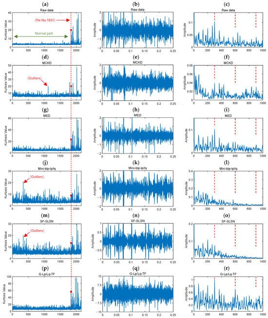
Figure 10.
Diagnosis results: (a,d,g,j,m,p) show the kurtosis variations over the full lifecycle for each method. (b,e,h,k,n,q) show the time-domain signals recovered after fault occurrence. (c,f,i,l,o,r) show the envelope spectra of the recovered signals post-fault. The red dots in the kurtosis variation plot indicate the kurtosis values at the moment of fault occurrence, while the red dashed line marks the reference line at 340 min. In the envelope spectrum, the red dashed lines represent the bearing fault frequency and its harmonics.
Table 6.
Earliest folders exhibiting abrupt kurtosis changes in the IMS dataset and their corresponding kurtosis values.
The filtered time-domain signals and envelope spectra following fault occurrence are plotted, with red dashed lines marking the bearing fault frequency and its harmonics, as shown in Figure 10. In the raw signal, only the fundamental fault frequency is discernible, while its harmonics are barely perceptible. In the cases of MCKD, Mini-blp-lplq, and SF-SLSN, fault features are not clearly visible, contributing minimally compared to the raw signal. Similarly, the MED reveals only the primary fault feature without a notable improvement over the raw signal. In contrast, the G-Lp/Lq-TF distinctly displays the fundamental fault frequency along with its harmonics, demonstrating its effectiveness in fault feature extraction. As shown in Table 7, the characteristic ratios of MCKD, MED, Mini-blp-lp/lq, and SF-SLSN are not higher than that of the raw data, indicating limited effectiveness in fault feature extraction. In contrast, the G-Lp/Lq-TF method achieves a characteristic ratio of 1.28%, representing a notable improvement over the raw data’s 1.06%. Overall, the G-Lp/Lq-TF exhibits strong stability in healthy bearings and effectively enhances fault feature extraction upon fault occurrence, outperforming existing mainstream methods.
Table 7.
Hilbert envelope spectrum fault feature ratio of IMS data.
4. Conclusions
This paper introduces a time and frequency domain blind deconvolution algorithm based on the generalized norm. By analyzing the limitations of applying the generalized norm separately in the time and frequency domains, appropriate parameter ranges are established to enable joint optimization across both domains. A joint optimization criterion is then formulated, ensuring that two opposing sparsity constraints interactively regulate the optimization process. Finally, experiments conducted on multiple signals validated the effectiveness of the proposed method.
- (1)
- To address the sensitivity of the generalized norm to noise spikes in the time domain and the loss of frequency components in the frequency domain, a blind deconvolution algorithm incorporating time and frequency domain optimization criteria is proposed. This method establishes a mutual constraint mechanism between time and frequency domain optimizations and employs deconvolution filters with backward automatic differentiation for gradient computation, effectively mitigating the limitations of the generalized norm when applied individually in each domain.
- (2)
- To overcome the lack of theoretical guidance in selecting appropriate and values for bearing fault sparsity analysis, the properties of the generalized norm in the sparse signal computation are derived and analyzed. The relationships between ratios, values, and signal sparsity are established, leading to the determination of optimal and values for both time and frequency domains, along with a reference framework for -value selection.
- (3)
- To validate the method’s effectiveness, experiments were conducted on simulated signals and three bearing fault datasets: CWRU, XJTU-SY, and IMS. In the synthetic signal experiments, the proposed method effectively extracted bearing fault features from strong noise interference. In the CWRU dataset experiments, the processed signal kurtosis values exceeded those of all other methods, confirming its superior sparsity performance. In the XJTU-SY and IMS dataset experiments, the proposed method demonstrated stability under healthy conditions and high sensitivity to faults, successfully extracting bearing fault frequencies from spindle rotation frequencies. The kurtosis values of G-Lp/Lq-TF at the anomaly points in the XJTU-SY and IMS datasets are 7.2573 and 58.2661, respectively, both exceeding those of other methods and the raw data. Its envelope spectrum fault feature ratios are 3.34% and 1.28%, respectively, also surpassing those of other methods and the raw data. These results demonstrate the superior effectiveness of this method in extracting fault features.
In conclusion, the time and frequency domain blind deconvolution method based on the generalized norm effectively extracts fault signal features across diverse scenarios. However, this study focuses on enhancing fault feature extraction in single-fault vibration signal diagnosis. The exploration of feature extraction techniques tailored to multi-failure scenarios presents a valuable direction for future research.
Author Contributions
Conceptualization, B.W. and Z.L.; methodology, B.W. and Z.L.; software, Z.L.; validation, B.W. and Z.L.; formal analysis, B.W. and J.Z.; investigation, J.Z.; resources, J.Z.; data curation, Z.L.; writing—original draft preparation, Z.L.; writing—review and editing, J.Z. and W.W; visualization, J.Z. and W.W.; supervision, B.W. and W.W.; project administration, B.W.; funding acquisition, B.W. All authors have read and agreed to the published version of the manuscript.
Funding
This research was funded by the Natural Science Foundation of China (Grant No. 52072116), the Key Research and Development Project of Hubei Province (Grant No. 2020BAB141), and the Special Fund of the Hubei Longzhong Laboratory of the Xiangyang Science and Technology Plan.
Data Availability Statement
The data supporting the conclusions of this article will be made available by the corresponding author upon request.
Conflicts of Interest
The authors declare no conflicts of interest.
Abbreviations
The following abbreviations are used in this manuscript:
| G-Lp/Lq-TF | Time and frequency domain blind deconvolution based on generalized norm |
| WT | Wavelet transform |
| VMD | Variational mode decomposition |
| BDMs | Blind deconvolution methods |
| LMD | Local mean decomposition |
| EMD | Empirical mode decomposition |
| SK | Spectral kurtosis |
| SVD | Singular value decomposition |
| MED | Minimum entropy deconvolution |
| MCKD | Maximum correlated kurtosis deconvolution |
| SHMD | Sparse maximum harmonics-to-noise-ratio deconvolution |
| CYCBD | Cyclostationarity blind deconvolution |
| OMED | Optimal minimum entropy deconvolution |
| SF-SLSN | Optimized minimum generalized deconvolution |
| Mini-blp-lplq | Prior-unknown blind deconvolution |
Appendix A
Case Western Reserve University (CWRU) Bearing Dataset [41]: The selected bearing type is a deep groove ball bearing, model 6205-2RS JEM SKF, with detailed parameters listed in Table A1. The vibration signal acquisition platform is illustrated in Figure A1.
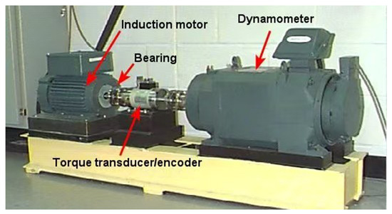
Figure A1.
CWRU vibration signal acquisition platform.
Table A1.
Specific parameters of CWRU bearings.
Table A1.
Specific parameters of CWRU bearings.
| Inside Diameter | Outside Diameter | Thickness | Ball Diameter | Pitch Diameter | |
|---|---|---|---|---|---|
| Size (inches) | 0.9843 | 2.0472 | 0.5906 | 0.3126 | 1.537 |
XJTU-SY Rolling Bearing Accelerated Degradation Dataset, provided by Xi’an Jiaotong University(XJTU), located in Xi’an, Shaanxi Province, China, and Changxing Shengyang Technology Co., Ltd. (SY), located in Zhejiang Province, China [42]: The bearing model used is LDK UER204, with detailed parameters listed in Table A2. The acceleration sensor is PCB 352C33. Figure A2 presents a photograph of the bearing fault.
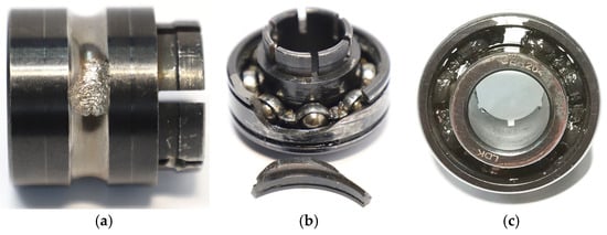
Figure A2.
Photograph of the bearing fault. (a) Inner race wear; (b) outer race fracture; (c) cage fracture.
Table A2.
Specific parameters of XJTU-SY bearings.
Table A2.
Specific parameters of XJTU-SY bearings.
| Outer Race Diameter/(mm) | Inner Race Diameter/(mm) | Bearing Mean Diameter/(mm) | Ball Diameter/(mm) | Number of Balls | |
|---|---|---|---|---|---|
| Parameter | 39.80 | 29.30 | 34.55 | 7.92 | 8 |
Full Lifecycle Bearing Dataset, provided by the Center for Intelligent Maintenance Systems (IMS) at the University of Cincinnati [44]: The bearing model used is Rexnord ZA-2115, with detailed parameters listed in Table A3. The acceleration sensor is PCB 353B33.
Table A3.
Specific parameters of IMS bearings.
Table A3.
Specific parameters of IMS bearings.
| Pitch Diameter/(Inches) | Roller Diameter/(Inches) | Tapered Contact Angle | Number of Rollers | |
|---|---|---|---|---|
| Parameter | 2.815 | 0.331 | 0.5906 | 32 |
Appendix B
The bearing fault characteristic frequencies are calculated as follows:
Fundamental Train Frequency (cage speed):
Ball Pass Frequency of the Outer Race:
Ball Pass Frequency of the Inner Race:
Ball(roller) Spin Frequency:
where is the shaft rotation speed, and denote the ball diameter and pitch diameter of the bearing, is the contact angle between the load and the radial plane, and represents the number of rolling elements.
References
- Miao, Y.H.; Zhang, B.Y.; Lin, J.; Zhao, M.; Liu, H.Y.; Liu, Z.Y.; Li, H. A review on the application of blind deconvolution in machinery fault diagnosis. Mech. Syst. Signal Process. 2022, 163, 108202. [Google Scholar] [CrossRef]
- Wei, Z.X.; He, D.Q.; Jin, Z.Z.; Liu, B.; Shan, S.; Chen, Y.J.; Miao, J. Density-Based affinity propagation tensor clustering for intelligent fault diagnosis of train bogie bearing. IEEE Trans. Intell. Transp. Syst. 2023, 24, 6053–6064. [Google Scholar] [CrossRef]
- Liu, X.Y.; Liu, S.L.; Xiang, J.W.; Sun, R.X. A transfer learning strategy based on numerical simulation driving 1D Cycle-GAN for bearing fault diagnosis. Inf. Sci. 2023, 642, 119175. [Google Scholar] [CrossRef]
- del Olmo, A.; López de Lacalle, L.N.; Martínez de Pissón, G.; Pérez-Salinas, C.; Ealo, J.A.; Sastoque, L.; Fernandes, M.H. Tool wear monitoring of high-speed broaching process with carbide tools to reduce production errors. Mech. Syst. Signal Process. 2022, 172, 109003. [Google Scholar] [CrossRef]
- Nazari, M.; Sakhaei, S.M. Successive variational mode decomposition. Signal Process. 2020, 174, 107610. [Google Scholar] [CrossRef]
- Zhao, Y.J.; Li, C.S.; Fu, W.L.; Liu, J.; Yu, T.; Chen, H. A modified variational mode decomposition method based on envelope nesting and multi-criteria evaluation. J. Sound Vib. 2020, 468, 115099. [Google Scholar] [CrossRef]
- Tang, J.H.; Wu, J.M.; Qing, J.J. A feature learning method for rotating machinery fault diagnosis via mixed pooling deep belief network and wavelet transform. Results Phys. 2022, 39, 105781. [Google Scholar] [CrossRef]
- Xu, Y.G.; Deng, Y.J.; Zhao, J.Y.; Tian, W.K.; Ma, C.Y. A novel rolling bearing fault diagnosis method based on empirical wavelet transform and spectral trend. IEEE Trans. Instrum. Meas. 2020, 69, 2891–2904. [Google Scholar] [CrossRef]
- Ruiz, P.; Zhou, X.; Mateos, J.; Molina, R.; Katsaggelos, A.K. Variational bayesian blind image deconvolution: A review. Digit. Signal Process. 2015, 47, 116–127. [Google Scholar] [CrossRef]
- Liu, Z.W.; He, Z.J.; Guo, W.; Tang, Z.C. A hybrid fault diagnosis method based on second generation wavelet de-noising and local mean decomposition for rotating machinery. ISA Trans. 2016, 61, 211–220. [Google Scholar] [CrossRef]
- Li, Y.B.; Liang, X.H.; Yang, Y.T.; Xu, M.Q.; Huang, W.H. Early fault diagnosis of rotating machinery by combining differential rational spline-based LMD and K-L divergence. IEEE Trans. Instrum. Meas. 2017, 66, 3077–3090. [Google Scholar] [CrossRef]
- Hoseinzadeh, M.S.; Khadem, S.E.; Sadooghi, M.S. Quantitative diagnosis for bearing faults by improving ensemble empirical mode decomposition. ISA Trans. 2018, 83, 261–275. [Google Scholar] [CrossRef] [PubMed]
- Li, Y.B.; Xu, M.Q.; Liang, X.H.; Huang, W.H. Application of bandwidth EMD and adaptive multiscale morphology analysis for incipient fault diagnosis of rolling bearings. IEEE Trans. Ind. Electron. 2017, 64, 6506–6517. [Google Scholar] [CrossRef]
- Wang, Y.X.; Xiang, J.W.; Markert, R.; Liang, M. Spectral kurtosis for fault detection, diagnosis and prognostics of rotating machines: A review with applications. Mech. Syst. Signal Process. 2016, 66–67, 679–698. [Google Scholar] [CrossRef]
- Lin, B.; Chang, P. Fault diagnosis of rolling element bearing using more robust spectral kurtosis and intrinsic time-scale decomposition. J. Vib. Control 2016, 22, 2921–2937. [Google Scholar] [CrossRef]
- Yu, M.Y.; Zhang, Y.; Yang, C.X. Rolling bearing faults identification based on multiscale singular value. Adv. Eng. Inform. 2023, 57, 102040. [Google Scholar] [CrossRef]
- Yu, T.Y.; Li, S.M.; Lu, J.T.; Gong, S.Q.; Gu, J.F.; Chen, Y. A quantum weak signal detection method for strengthening target signal features under strong white gaussian noise. Appl. Sci. 2022, 12, 1878. [Google Scholar] [CrossRef]
- Wang, Z.J.; Zhou, J.; Du, W.H.; Lei, Y.G.; Wang, J.Y. Bearing fault diagnosis method based on adaptive maximum cyclostationarity blind deconvolution. Mech. Syst. Signal Process. 2022, 162, 108018. [Google Scholar] [CrossRef]
- McDonald, G.L.; Zhao, Q. Multipoint optimal minimum entropy deconvolution and convolution fix: Application to vibration fault detection. Mech. Syst. Signal Process. 2017, 82, 461–477. [Google Scholar] [CrossRef]
- López, C.; Wang, D.; Naranjo, Á.; Moore, K.J. Box-cox-sparse-measures-based blind filtering: Understanding the difference between the maximum kurtosis deconvolution and the minimum entropy deconvolution. Mech. Syst. Signal Process. 2022, 165, 108376. [Google Scholar] [CrossRef]
- Wiggins, R.A. Minimum entropy deconvolution. Geoexploration 1978, 16, 21–35. [Google Scholar] [CrossRef]
- McDonald, G.L.; Zhao, Q.; Zuo, M.J. Maximum correlated Kurtosis deconvolution and application on gear tooth chip fault detection. Mech. Syst. Signal Process. 2012, 33, 237–255. [Google Scholar] [CrossRef]
- Miao, Y.H.; Zhao, M.; Lin, J.; Xu, X.Q. Sparse maximum harmonics-to-noise-ratio deconvolution for weak fault signature detection in bearings. Meas. Sci. Technol. 2016, 27, 105004. [Google Scholar] [CrossRef]
- Miao, Y.H.; Zhao, M.; Lin, J.; Liang, K.X.; Liu, G. Harmonics-to-noise ratio guided deconvolution and its application for bearing fault detection. In Proceedings of the 2017 Prognostics and System Health Management Conference (PHM-Harbin), Harbin, China, 9–12 July 2017; pp. 1–8. [Google Scholar] [CrossRef]
- Karioja, K.; Nikula, R.P.; Nissilä, J. Cyclostationarity and real order derivatives in roller bearing fault detection. Meas. Sci. Technol. 2024, 35, 096136. [Google Scholar] [CrossRef]
- Jia, X.D.; Zhao, M.; Buzza, M.; Di, Y.; Lee, J. A geometrical investigation on the generalized lp/lq norm for blind deconvolution. Signal Process. 2017, 134, 63–69. [Google Scholar] [CrossRef]
- He, L.; Yi, C.; Wang, D.; Wang, F.; Lin, J.H. Optimized minimum generalized Lp/Lq deconvolution for recovering repetitive impacts from a vibration mixture. Measurement 2021, 168, 108329. [Google Scholar] [CrossRef]
- He, L.; Wang, D.; Yi, C.; Zhou, Q.Y.; Lin, J.H. Extracting cyclo-stationarity of repetitive transients from envelope spectrum based on prior-unknown blind deconvolution technique. Signal Process. 2021, 183, 107997. [Google Scholar] [CrossRef]
- Cao, W.P.; Li, H.H.; Hu, C.G.; Wang, H.; Huang, R.Q.; Lu, S.L.; Huang, X.Y. Diagnosis of high-resistance connection faults in PMSMs based on GMR and deep learning. IEEE Trans. Ind. Electron. 2024, 71, 7915–7923. [Google Scholar] [CrossRef]
- Guo, J.Y.; Wang, Z.Y.; Li, H.; Yang, Y.L.; Huang, C.G.; Yazdi, M.; Kang, H.S. A hybrid prognosis scheme for rolling bearings based on a novel health indicator and nonlinear Wiener process. Reliab. Eng. Syst. Saf. 2024, 245, 110014. [Google Scholar] [CrossRef]
- Wang, B.H.; Zhang, J.C.; Wang, W.L.; Cheng, T.T. Fractional Diversity Entropy: A vibration signal measure to assist a diffusion model in the fault diagnosis of automotive machines. Electronics 2024, 13, 3155. [Google Scholar] [CrossRef]
- Zhou, Q.D.; Zhang, J.H.; Zhou, T.Y.; Qiu, Y.B.; Jia, H.J.; Lin, J.W. A parameter-adaptive variational mode decomposition approach based on weighted fuzzy-distribution entropy for noise source separation. Meas. Sci. Technol. 2020, 31, 125004. [Google Scholar] [CrossRef]
- Ding, C.C.; Zhao, M.; Lin, J. Sparse feature extraction based on periodical convolutional sparse representation for fault detection of rotating machinery. Meas. Sci. Technol. 2021, 32, 015008. [Google Scholar] [CrossRef]
- Gray, W. Variable Norm Deconvolution. Ph.D. Thesis, Stanford University, Stanford, CA, USA, 1979. [Google Scholar]
- Hurley, N.; Rickard, S. Comparing measures of sparsity. IEEE Trans. Inf. Theory 2009, 55, 4723–4741. [Google Scholar] [CrossRef]
- Liao, J.X.; He, C.; Li, J.P.; Sun, J.W.; Zhang, S.P.; Zhang, X.G. Classifier-guided neural blind deconvolution: A physics-informed denoising module for bearing fault diagnosis under noisy conditions. Mech. Syst. Signal Process. 2025, 222, 111750. [Google Scholar] [CrossRef]
- Zhao, M.; Lin, J.; Miao, Y.H.; Xu, X.Q. Detection and recovery of fault impulses via improved harmonic product spectrum and its application in defect size estimation of train bearings. Measurement 2016, 91, 421–439. [Google Scholar] [CrossRef]
- Aurrekoetxea, M.; de Lacalle, L.N.L.; Zelaieta, O.; Llanos, I. In-process machining distortion prediction method based on bulk residual stresses estimation from reduced layer removal. J. Manuf. Mater. Process. 2024, 8, 9. [Google Scholar] [CrossRef]
- López de Lacalle, L.N.; Lamikiz, A.; Sánchez, J.A.; Fernández de Bustos, I. Recording of real cutting forces along the milling of complex parts. Mechatronics 2006, 16, 21–32. [Google Scholar] [CrossRef]
- López de Lacalle, L.N.; Lamikiz, A.; Sanchez, J.A.; de Bustos, I.F. Simultaneous measurement of forces and machine tool position for diagnostic of machining tests. IEEE Trans. Instrum. Meas. 2005, 54, 2329–2335. [Google Scholar] [CrossRef]
- Bearing Data Center, Case Western Reserve University. Available online: https://engineering.case.edu/bearingdatacenter/welcome (accessed on 6 January 2025).
- Wang, P.; Long, Z.Q.; Wang, G. A hybrid prognostics approach for estimating remaining useful life of wind turbine bearings. Energy Rep. 2020, 6, 173–182. [Google Scholar] [CrossRef]
- He, W.P.; Zi, Y.Y.; Chen, B.Q.; Wu, F.; He, Z.J. Automatic fault feature extraction of mechanical anomaly on induction motor bearing using ensemble super-wavelet transform. Mech. Syst. Signal Process. 2015, 54–55, 457–480. [Google Scholar] [CrossRef]
- Qiu, H.; Lee, J.; Lin, J.; Yu, G. Wavelet filter-based weak signature detection method and its application on rolling element bearing prognostics. J. Sound Vib. 2006, 289, 1066–1090. [Google Scholar] [CrossRef]
Disclaimer/Publisher’s Note: The statements, opinions and data contained in all publications are solely those of the individual author(s) and contributor(s) and not of MDPI and/or the editor(s). MDPI and/or the editor(s) disclaim responsibility for any injury to people or property resulting from any ideas, methods, instructions or products referred to in the content. |
© 2025 by the authors. Licensee MDPI, Basel, Switzerland. This article is an open access article distributed under the terms and conditions of the Creative Commons Attribution (CC BY) license (https://creativecommons.org/licenses/by/4.0/).