
FSFF-Net: A Frequency-Domain Feature and Spatial-Domain Feature Fusion Network for Hyperspectral Image Classification


Abstract

1. Introduction
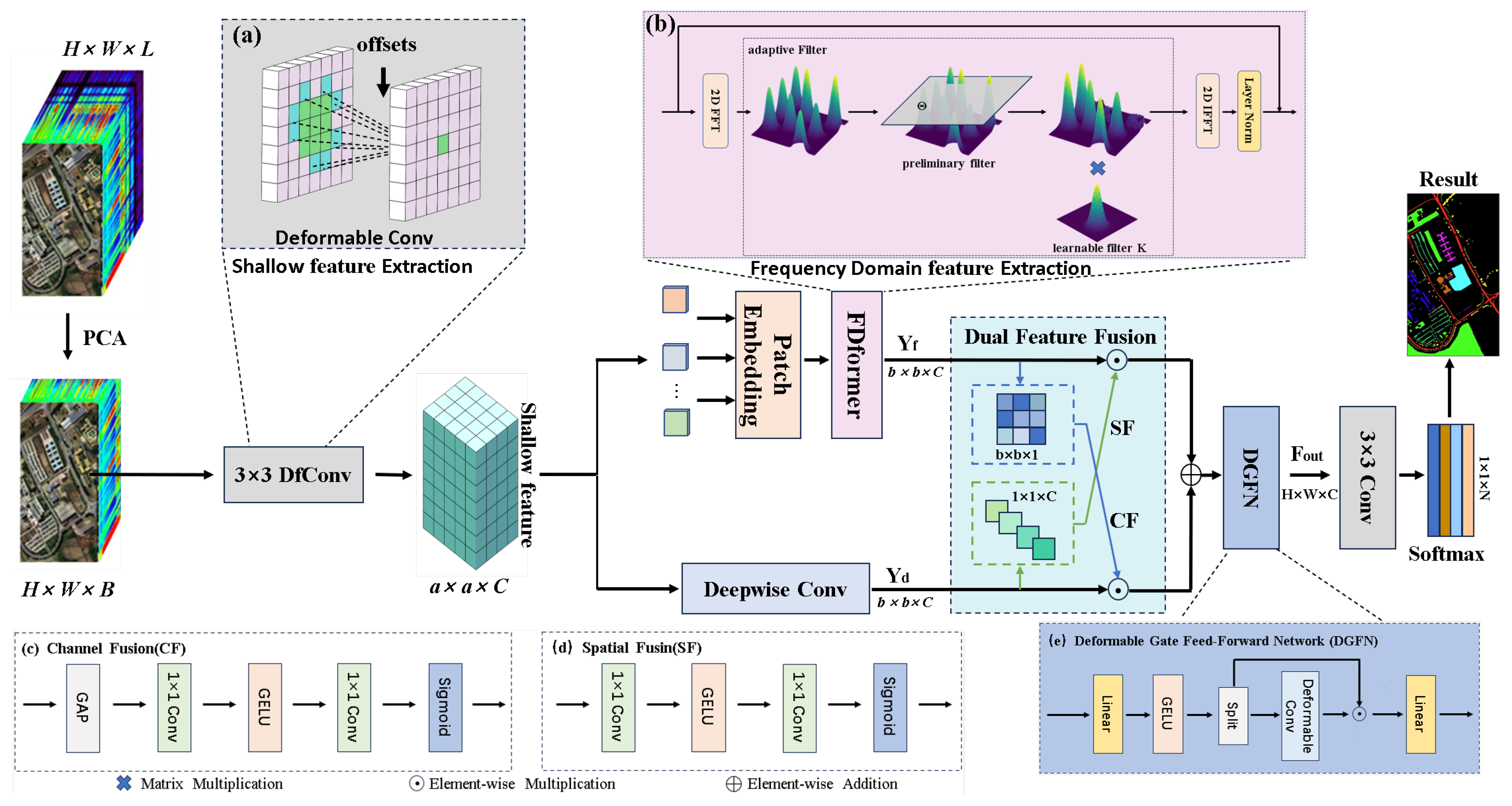
- We propose a novel module, the FDformer, for capturing frequency-domain features. This module not only reduces computational overhead by decreasing the number of parameters, but also overcomes the limitations of CNN by capturing complementary frequency-domain features, which enhance the spatial-domain features for improved classification. It takes the place of the self-attention layer in visual transformers with three steps: two-dimensional discrete Fourier transform, adaptive filter, and two-dimensional inverse Fourier transform. We proved in the subsequent ablation experiments that FDformer effectively captures frequency domain features and improves classification accuracy.
- We propose a novel module, a deformable gate feed-forward network (DGFN) to feature refinement. The traditional FFN [53] neglects the modeling of spatial information. Additionally, redundant information in the channels affects the expressive power of the features and it cannot adapt to local deformations. We replaced the conv module in the FFN with a gating mechanism based on deformable convolution. We demonstrate in the subsequent ablation experiments that DGFN is capable of capturing spatial information and further fitting class shapes, improving classification accuracy.
- We propose a dual-domain feature fusion network for HSI classification. The network integrates frequency domain features and spatial features, enhancing classification accuracy and the robustness of the network. An image after deformable convolution is passed through both the FDformer module and the deepwise convolution module. Then, the feature fusion module allows sufficient interaction between the frequency-domain and spatial-domain feature in HSI. Finally, these features are further refined through the deformable gate feed-forward network, further enhancing classification accuracy. The experimental results across four public datasets confirm the advantages of the proposed network.
2. Materials and Methods
2.1. Network Framework
2.2. Frequency Domain Transformer
2.3. Dual Feature Fusion (DFF)
2.4. Deformable Gate Feed-Forward Network
3. Results
3.1. Data Description
3.2. Experimental Setting
- Evaluation metrics: To evaluate the performance of the proposed model on the four different datasets, four common HSI classification evaluation metrics were used: overall accuracy (OA), average accuracy (AA), kappa coefficient, and F1 score. The overall accuracy (OA) is calculated as the percentage of properly classified pixels and is used to measure the overall performance of the classification model on the entire dataset. Average accuracy (AA) is calculated as the mean percentage of correctly classified pixels for each class and is employed to evaluate the proficiency of the model across all individual classes. The kappa coefficient serves as a quantitative metric calculated from the confusion matrix, which quantifies the correlation between the predicted and correct labels. The F1 score is the harmonic mean for measuring the precision and recall in the classification model, used to balance the performance of both.
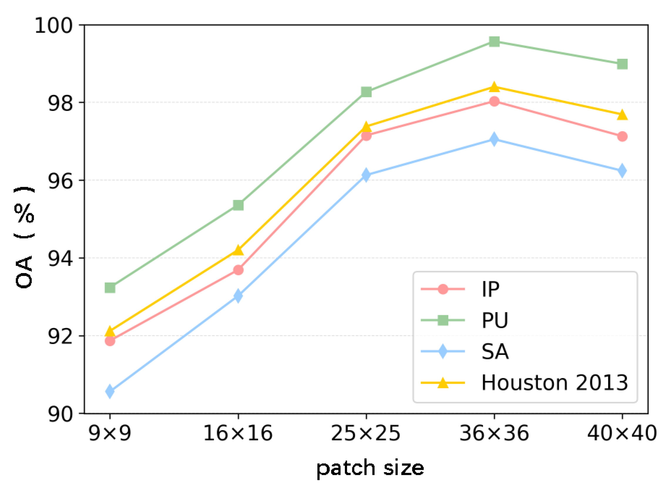
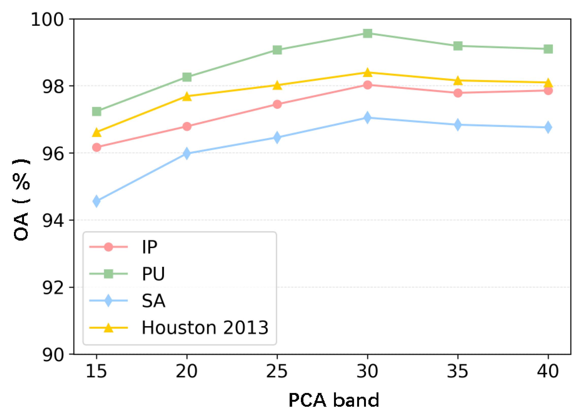
- Configuration: In the experiment, the quantity of hyperspectral image bands after PCA dimensionality reduction, symbolized by C, is set to 30. The 3D block size is 36 × 36, and the embedding block size is 6 × 6. The Adam optimizer with a learning rate of 0.001 is utilized for training the model. For batch training, the batch size is set to 256. The training is run through 100 epochs. The experimental hardware environment consists of an i7-10500 CPU and an NVIDIA GeForce RTX 4090 GPU, with our compilation environment being Python 3.8 and Pytorch 1.11.0.
3.3. Comparative Experimentation
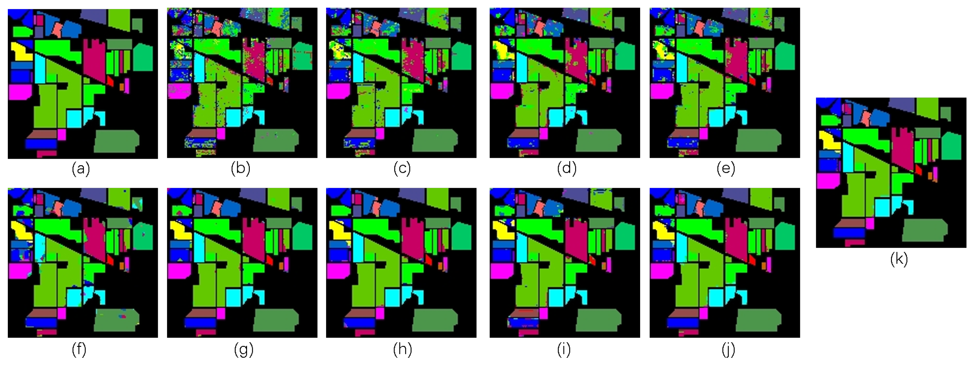
3.3.1. Experiment on the IP
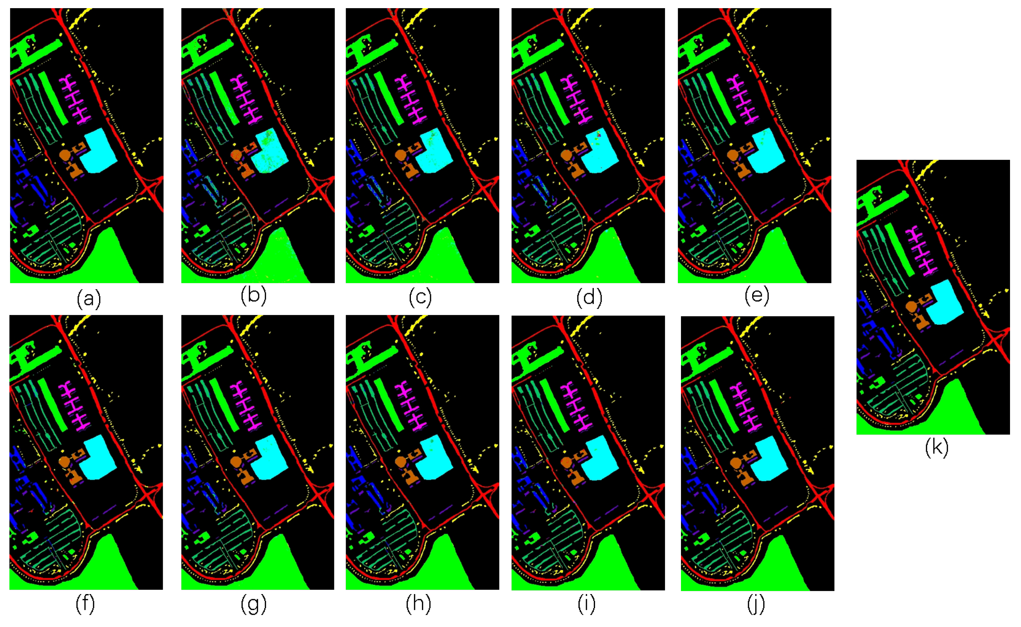
3.3.2. Experiment on the PU
3.3.3. Experiment on the Salinas Scene Dataset
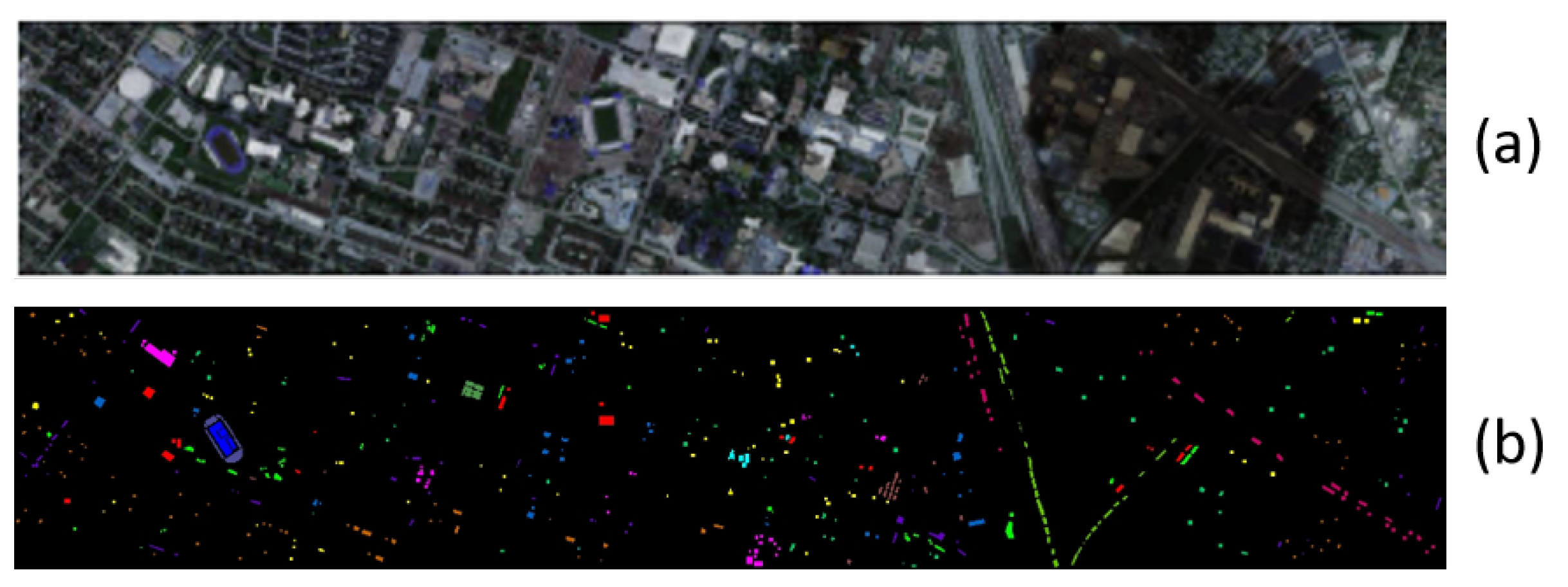
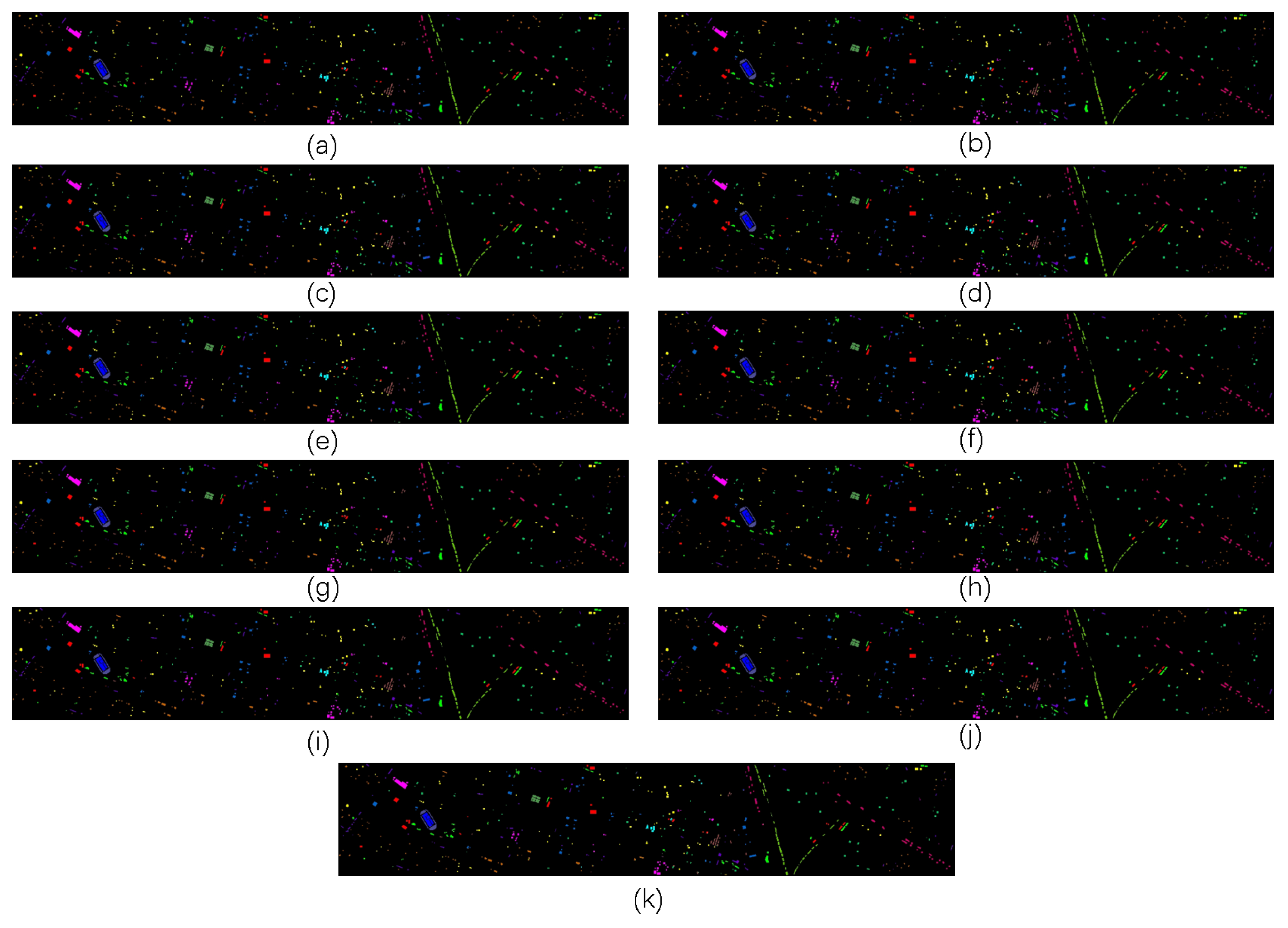
3.3.4. Experiment on the Houston 2013 Dataset
3.4. Ablation Study
3.5. Parameter Study
3.6. Memory and Time
3.7. Comparison of Classification Accuracy Under Different Training Sample Ratio
4. Limitations and Discussion
5. Conclusions
Author Contributions
Funding
Data Availability Statement
Conflicts of Interest
References
- Zhang, Q.; Zheng, Y.; Yuan, Q.; Song, M.; Yu, H.; Xiao, Y. Hyperspectral image denoising: From model-driven, data-driven, to model-data-driven. IEEE Trans. Neural Netw. Learn. Syst. 2023, 35, 13143–13163. [Google Scholar] [CrossRef] [PubMed]
- Huo, Y.; Cheng, X.; Lin, S.; Zhang, M.; Wang, H. Memory-augmented Autoencoder with Adaptive Reconstruction and Sample Attribution Mining for Hyperspectral Anomaly Detection. IEEE Trans. Geosci. Remote Sens. 2024, 62, 5518118. [Google Scholar] [CrossRef]
- Cheng, X.; Zhang, M.; Lin, S.; Li, Y.; Wang, H. Deep self-representation learning framework for hyperspectral anomaly detection. IEEE Trans. Instrum. Meas. 2023, 73, 5002016. [Google Scholar] [CrossRef]
- Liu, X.; Jiao, L.; Li, L.; Tang, X.; Guo, Y. Deep multi-level fusion network for multi-source image pixel-wise classification. Knowl.-Based Syst. 2021, 221, 106921. [Google Scholar] [CrossRef]
- Noor, S.S.M.; Michael, K.; Marshall, S.; Ren, J.; Tschannerl, J.; Kao, F.J. The properties of the cornea based on hyperspectral imaging: Optical biomedical engineering perspective. In Proceedings of the 2016 International Conference on Systems, Signals and Image Processing (IWSSIP), Bratislava, Slovakia, 23–25 May 2016; pp. 1–4. [Google Scholar] [CrossRef]
- Wang, J.; Zhang, L.; Tong, Q.; Sun, X. The Spectral Crust project—Research on new mineral exploration technology. In Proceedings of the 2012 4th Workshop on Hyperspectral Image and Signal Processing: Evolution in Remote Sensing (WHISPERS), Shanghai, China, 4–7 June 2012; pp. 1–4. [Google Scholar] [CrossRef]
- Fong, A.; Shu, G.; McDonogh, B. Farm to table: Applications for new hyperspectral imaging technologies in precision agriculture, food quality and safety. In Proceedings of the Conference on Lasers and Electro-Optics, San Jose, CA, USA, 10–15 May 2020; p. AW3K.2. [Google Scholar] [CrossRef]
- Ardouin, J.P.; Lévesque, J.; Rea, T.A. A demonstration of hyperspectral image exploitation for military applications. In Proceedings of the 2007 10th International Conference on Information Fusion, Quebec, QC, Canada, 9–12 July 2007; pp. 1–8. [Google Scholar] [CrossRef]
- Sun, L.; He, C.; Zheng, Y.; Tang, S. SLRL4D: Joint Restoration of S ubspace L ow-R ank L earning and Non-Local 4-D Transform Filtering for Hyperspectral Image. Remote Sens. 2020, 12, 2979. [Google Scholar] [CrossRef]
- He, C.; Sun, L.; Huang, W.; Zhang, J.; Zheng, Y.; Jeon, B. TSLRLN: Tensor subspace low-rank learning with non-local prior for hyperspectral image mixed denoising. Signal Process. 2021, 184, 108060. [Google Scholar] [CrossRef]
- Sun, L.; Wu, F.; Zhan, T.; Liu, W.; Wang, J.; Jeon, B. Weighted nonlocal low-rank tensor decomposition method for sparse unmixing of hyperspectral images. IEEE J. Sel. Top. Appl. Earth Obs. Remote Sens. 2020, 13, 1174–1188. [Google Scholar] [CrossRef]
- Yang, S.; Shi, Z. Hyperspectral image target detection improvement based on total variation. IEEE Trans. Image Process. 2016, 25, 2249–2258. [Google Scholar] [CrossRef]
- Sun, L.; Wu, Z.; Liu, J.; Xiao, L.; Wei, Z. Supervised spectral–spatial hyperspectral image classification with weighted Markov random fields. IEEE Trans. Geosci. Remote Sens. 2014, 53, 1490–1503. [Google Scholar] [CrossRef]
- Sun, L.; Ma, C.; Chen, Y.; Zheng, Y.; Shim, H.J.; Wu, Z.; Jeon, B. Low rank component induced spatial-spectral kernel method for hyperspectral image classification. IEEE Trans. Circuits Syst. Video Technol. 2019, 30, 3829–3842. [Google Scholar] [CrossRef]
- Chen, M.; Feng, S.; Zhao, C.; Qu, B.; Su, N.; Li, W.; Tao, R. Fractional Fourier Based Frequency-Spatial-Spectral Prototype Network for Agricultural Hyperspectral Image Open-Set Classification. IEEE Trans. Geosci. Remote Sens. 2024, 62, 5514014. [Google Scholar] [CrossRef]
- Lv, Z.; Li, G.; Jin, Z.; Benediktsson, J.A.; Foody, G.M. Iterative training sample expansion to increase and balance the accuracy of land classification from VHR imagery. IEEE Trans. Geosci. Remote Sens. 2020, 59, 139–150. [Google Scholar] [CrossRef]
- Fauvel, M.; Benediktsson, J.A.; Chanussot, J.; Sveinsson, J.R. Spectral and spatial classification of hyperspectral data using SVMs and morphological profiles. IEEE Trans. Geosci. Remote Sens. 2008, 46, 3804–3814. [Google Scholar] [CrossRef]
- Benediktsson, J.A.; Palmason, J.A.; Sveinsson, J.R. Classification of hyperspectral data from urban areas based on extended morphological profiles. IEEE Trans. Geosci. Remote Sens. 2005, 43, 480–491. [Google Scholar] [CrossRef]
- Tang, Y.; Feng, S.; Zhao, C.; Fan, Y.; Shi, Q.; Li, W.; Tao, R. An object fine-grained change detection method based on frequency decoupling interaction for high-resolution remote sensing images. IEEE Trans. Geosci. Remote Sens. 2023, 62, 5600213. [Google Scholar] [CrossRef]
- Sun, L.; Ma, C.; Chen, Y.; Shim, H.J.; Wu, Z.; Jeon, B. Adjacent superpixel-based multiscale spatial-spectral kernel for hyperspectral classification. IEEE J. Sel. Top. Appl. Earth Obs. Remote Sens. 2019, 12, 1905–1919. [Google Scholar] [CrossRef]
- Chen, Y.; Lin, Z.; Zhao, X.; Wang, G.; Gu, Y. Deep learning-based classification of hyperspectral data. IEEE J. Sel. Top. Appl. Earth Obs. Remote Sens. 2014, 7, 2094–2107. [Google Scholar] [CrossRef]
- Chen, Y.; Zhao, X.; Jia, X. Spectral–spatial classification of hyperspectral data based on deep belief network. IEEE J. Sel. Top. Appl. Earth Obs. Remote Sens. 2015, 8, 2381–2392. [Google Scholar] [CrossRef]
- Krizhevsky, A.; Sutskever, I.; Hinton, G.E. Imagenet classification with deep convolutional neural networks. Adv. Neural Inf. Process. Syst. 2017, 60, 84–90. [Google Scholar] [CrossRef]
- Lin, M. Network in network. arXiv 2013, arXiv:1312.4400. [Google Scholar] [CrossRef]
- He, K.; Zhang, X.; Ren, S.; Sun, J. Deep Residual Learning for Image Recognition. 2016, pp. 770–778. Available online: https://openaccess.thecvf.com/content_cvpr_2016/html/He_Deep_Residual_Learning_CVPR_2016_paper.html (accessed on 15 December 2024).
- Zhong, Z.; Li, J.; Luo, Z.; Chapman, M. Spectral–spatial residual network for hyperspectral image classification: A 3-D deep learning framework. IEEE Trans. Geosci. Remote Sens. 2017, 56, 847–858. [Google Scholar] [CrossRef]
- Roy, S.K.; Krishna, G.; Dubey, S.R.; Chaudhuri, B.B. HybridSN: Exploring 3-D–2-D CNN feature hierarchy for hyperspectral image classification. IEEE Geosci. Remote Sens. Lett. 2019, 17, 277–281. [Google Scholar] [CrossRef]
- Wang, J.; Song, X.; Sun, L.; Huang, W.; Wang, J. A novel cubic convolutional neural network for hyperspectral image classification. IEEE J. Sel. Top. Appl. Earth Obs. Remote Sens. 2020, 13, 4133–4148. [Google Scholar] [CrossRef]
- Zheng, Y.; Liu, S.; Bruzzone, L. An Attention-Enhanced Feature Fusion Network (AeF 2 N) for Hyperspectral Image Classification. IEEE Geosci. Remote Sens. Lett. 2023, 20, 5511005. [Google Scholar] [CrossRef]
- Yu, C.; Zhao, X.; Gong, B.; Hu, Y.; Song, M.; Yu, H.; Chang, C.I. Distillation-constrained prototype representation network for hyperspectral image incremental classification. IEEE Trans. Geosci. Remote Sens. 2024, 62, 5507414. [Google Scholar] [CrossRef]
- Zhang, Q.; Dong, Y.; Yuan, Q.; Song, M.; Yu, H. Combined deep priors with low-rank tensor factorization for hyperspectral image restoration. IEEE Geosci. Remote Sens. Lett. 2023, 20, 5500205. [Google Scholar] [CrossRef]
- Dosovitskiy, A. An image is worth 16x16 words: Transformers for image recognition at scale. arXiv 2020, arXiv:2010.11929. [Google Scholar]
- Sun, Q.; Sun, Y.; Pan, C. AIDB-Net: An Attention-Interactive Dual-Branch Convolutional Neural Network for Hyperspectral Pansharpening. Remote Sens. 2024, 16, 1044. [Google Scholar] [CrossRef]
- Touvron, H.; Cord, M.; Douze, M.; Massa, F.; Sablayrolles, A.; Jégou, H. Training data-efficient image transformers & distillation through attention. In Proceedings of the 38th International Conference on Machine Learning, Virtual, 18–24 July 2021; pp. 10347–10357. [Google Scholar]
- He, X.; Chen, Y.; Lin, Z. Spatial-spectral transformer for hyperspectral image classification. Remote Sens. 2021, 13, 498. [Google Scholar] [CrossRef]
- Simonyan, K. Very deep convolutional networks for large-scale image recognition. arXiv 2014, arXiv:1409.1556. [Google Scholar]
- Hong, D.; Han, Z.; Yao, J.; Gao, L.; Zhang, B.; Plaza, A.; Chanussot, J. SpectralFormer: Rethinking hyperspectral image classification with transformers. IEEE Trans. Geosci. Remote Sens. 2021, 60, 5518615. [Google Scholar] [CrossRef]
- He, X.; Zhou, Y.; Zhao, J.; Zhang, D.; Yao, R.; Xue, Y. Swin transformer embedding UNet for remote sensing image semantic segmentation. IEEE Trans. Geosci. Remote Sens. 2022, 60, 4408715. [Google Scholar] [CrossRef]
- Jiang, M.; Su, Y.; Gao, L.; Plaza, A.; Zhao, X.L.; Sun, X.; Liu, G. GraphGST: Graph generative structure-aware transformer for hyperspectral image classification. IEEE Trans. Geosci. Remote Sens. 2024, 62, 5504016. [Google Scholar] [CrossRef]
- Wang, D.; Zhuang, L.; Gao, L.; Sun, X.; Zhao, X.; Plaza, A. Sliding dual-window-inspired reconstruction network for hyperspectral anomaly detection. IEEE Trans. Geosci. Remote Sens. 2024, 62, 5504115. [Google Scholar] [CrossRef]
- Xiang, P.; Ali, S.; Zhang, J.; Jung, S.K.; Zhou, H. Pixel-associated autoencoder for hyperspectral anomaly detection. Int. J. Appl. Earth Obs. Geoinf. 2024, 129, 103816. [Google Scholar] [CrossRef]
- Pitas, I. Digital Image Processing Algorithms and Applications; John Wiley & Sons Inc.: Hoboken, NJ, USA, 2000; Volume 2, pp. 133–138. Available online: https://books.google.com.tw/books?hl=zh-CN&lr=&id=VQs_Ly4DYDMC&oi=fnd&pg=PA1&dq=Ioannis+Pitas.+Digital+image+processing+algorithms+and+applications.+John+Wiley+Sons,+200&ots=jKofgIqfZp&sig=-SilbYomsMP1YkRBc9kptzRAJTg&redir_esc=y#v=onepage&q=Ioannis%20Pitas.%20Digital%20image%20processing%20algorithms%20and%20applications.%20John%20Wiley%20Sons%2C%20200&f=false (accessed on 15 December 2024).
- Baxes, G.A. Digital Image Processing: Principles and Applications; John Wiley & Sons, Inc.: Hoboken, NJ, USA, 1994. [Google Scholar]
- Song, G.; Sun, Q.; Zhang, L.; Su, R.; Shi, J.; He, Y. OPE-SR: Orthogonal position encoding for designing a parameter-free upsampling module in arbitrary-scale image super-resolution. In Proceedings of the 2023 IEEE/CVF Conference on Computer Vision and Pattern Recognition (CVPR), Vancouver, BC, Canada, 18–22 June 2023; pp. 10009–10020. [Google Scholar] [CrossRef]
- Li, S.; Xue, K.; Zhu, B.; Ding, C.; Gao, X.; Wei, D.; Wan, T. Falcon: A fourier transform based approach for fast and secure convolutional neural network predictions. In Proceedings of the IEEE/CVF Conference on Computer Vision and Pattern Recognition, Seattle, WA, USA, 13–19 June 2020; pp. 8705–8714. Available online: https://openaccess.thecvf.com/content_CVPR_2020/html/Li_FALCON_A_Fourier_Transform_Based_Approach_for_Fast_and_Secure_CVPR_2020_paper.html (accessed on 15 December 2024).
- Yang, Y.; Soatto, S. Fda: Fourier domain adaptation for semantic segmentation. In Proceedings of the IEEE/CVF Conference on Computer Vision and Pattern Recognition, Seattle, WA, USA, 13–19 June 2020; pp. 4085–4095. Available online: https://openaccess.thecvf.com/content_CVPR_2020/html/Yang_FDA_Fourier_Domain_Adaptation_for_Semantic_Segmentation_CVPR_2020_paper.html (accessed on 20 December 2024).
- Ding, C.; Liao, S.; Wang, Y.; Li, Z.; Liu, N.; Zhuo, Y.; Wang, C.; Qian, X.; Bai, Y.; Yuan, G.; et al. Circnn: Accelerating and compressing deep neural networks using block-circulant weight matrices. In Proceedings of the 50th Annual IEEE/ACM International Symposium on Microarchitecture, Cambridge, MA, USA, 14–18 October 2017; pp. 395–408. [Google Scholar] [CrossRef]
- Chi, L.; Jiang, B.; Mu, Y. Fast fourier convolution. Adv. Neural Inf. Process. Syst. 2020, 33, 4479–4488. [Google Scholar]
- Rao, Y.; Zhao, W.; Zhu, Z.; Lu, J.; Zhou, J. Global filter networks for image classification. Adv. Neural Inf. Process. Syst. 2021, 34, 980–993. [Google Scholar]
- Lee, J.H.; Heo, M.; Kim, K.R.; Kim, C.S. Single-image depth estimation based on fourier domain analysis. In Proceedings of the 2018 IEEE/CVF Conference on Computer Vision and Pattern Recognition, Salt Lake City, UT, USA, 18–23 June 2018; pp. 330–339. Available online: https://openaccess.thecvf.com/content_cvpr_2018/html/Lee_Single-Image_Depth_Estimation_CVPR_2018_paper.html (accessed on 20 December 2024).
- Rao, Y.; Zhao, W.; Zhu, Z.; Lu, J.; Zhou, J. Global Filter Networks for Image Classification. arXiv 2021, arXiv:2107.00645. [Google Scholar] [CrossRef]
- Zhu, X.; Hu, H.; Lin, S.; Dai, J. Deformable convnets v2: More deformable, better results. In Proceedings of the 2019 IEEE/CVF Conference on Computer Vision and Pattern Recognition (CVPR), Long Beach, CA, USA, 15–20 June 2019; pp. 9308–9316. Available online: https://openaccess.thecvf.com/content_CVPR_2019/html/Zhu_Deformable_ConvNets_V2_More_Deformable_Better_Results_CVPR_2019_paper.html (accessed on 5 December 2024).
- Ashish, V. Attention is all you need. Adv. Neural Inf. Process. Syst. 2017, 30, I. [Google Scholar]
- USGS. Hyperspectral Image Data Set: Indian Pines. In Proceedings of the AVIRIS Sensor Data Products. 1992. Available online: https://www.ehu.eus/ccwintco/index.php/Hyperspectral_Remote_Sensing_Scenes (accessed on 10 October 2024).
- DLR. Hyperspectral Image Data Set: University of Pavia. In Proceedings of the ROSIS-03 Sensor Data Products. 2003. Available online: https://www.ehu.eus/ccwintco/index.php/Hyperspectral_Remote_Sensing_Scenes (accessed on 10 October 2024).
- USGS. Hyperspectral Image Data Set: Salinas. In Proceedings of the A VIRIS Sensor Data Products. 1992. Available online: https://www.ehu.eus/ccwintco/index.php/Hyperspectral_Remote_Sensing_Scenes (accessed on 10 October 2024).
- Gader, P.; Zare, A.; Close, R.; Aitken, J.; Tuell, G. MU UFL Gulfport Hyperspectral and LiDAR Airborne Data Set; Technical Report Rep-2013-570; University of Florida: Gainesville, FL, USA, 2013; Available online: https://hyperspectral.ee.uh.edu/?page_id=459 (accessed on 5 December 2024).
- Hu, W.; Huang, Y.; Wei, L.; Zhang, F.; Li, H. Deep convolutional neural networks for hyperspectral image classification. J. Sens. 2015, 2015, 258619. [Google Scholar] [CrossRef]
- Zhao, W.; Du, S. Spectral–spatial feature extraction for hyperspectral image classification: A dimension reduction and deep learning approach. IEEE Trans. Geosci. Remote Sens. 2016, 54, 4544–4554. [Google Scholar] [CrossRef]
- Yue, J.; Zhao, W.; Mao, S.; Liu, H. Spectral–spatial classification of hyperspectral images using deep convolutional neural networks. Remote Sens. Lett. 2015, 6, 468–477. [Google Scholar] [CrossRef]
- Chen, Y.; Jiang, H.; Li, C.; Jia, X.; Ghamisi, P. Deep feature extraction and classification of hyperspectral images based on convolutional neural networks. IEEE Trans. Geosci. Remote Sens. 2016, 54, 6232–6251. [Google Scholar] [CrossRef]
- Sun, L.; Zhao, G.; Zheng, Y.; Wu, Z. Spectral–spatial feature tokenization transformer for hyperspectral image classification. IEEE Trans. Geosci. Remote Sens. 2022, 60, 5522214. [Google Scholar] [CrossRef]
- Qiao, X.; Huang, W. Spectral-Spatial-Frequency Transformer Network for Hyperspectral Image Classification. In Proceedings of the 2023 IEEE Sensors Applications Symposium (SAS), Ottawa, ON, Canada, 18–20 July 2023. [Google Scholar] [CrossRef]
- Yu, C.; Zhu, Y.; Song, M.; Wang, Y.; Zhang, Q. Unseen feature extraction: Spatial mapping expansion with spectral compression network for hyperspectral image classification. IEEE Trans. Geosci. Remote Sens. 2024, 62, 5521915. [Google Scholar] [CrossRef]
- Roy, S.K.; Deria, A.; Shah, C.; Haut, J.M.; Du, Q.; Plaza, A. Spectral–Spatial Morphological Attention Transformer for Hyperspectral Image Classification. IEEE Trans. Geosci. Remote Sens. 2023, 61, 5503615. [Google Scholar] [CrossRef]
- Jin, M.; Li, K.; Li, S.; He, C.; Li, X. Towards Realizing the Value of Labeled Target Samples: A Two-Stage Approach for Semi-Supervised Domain Adaptation. In Proceedings of the ICASSP 2023—2023 IEEE International Conference on Acoustics, Speech and Signal Processing (ICASSP), Rhodes Island, Greece, 4–10 June 2023. [Google Scholar] [CrossRef]


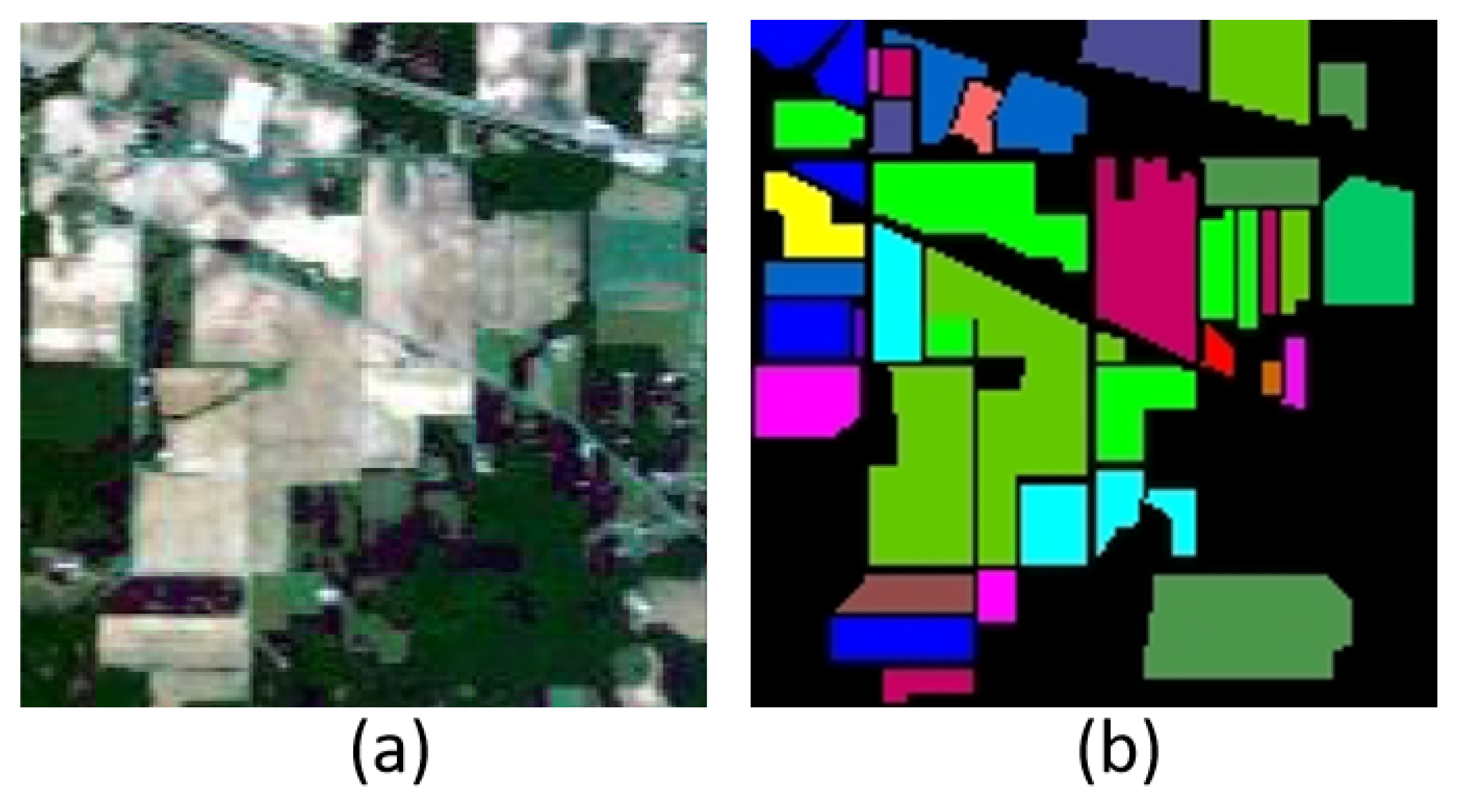
| No. | Class Name | Training | Testing | Total |
|---|---|---|---|---|
| 1 | Alfalfa | 5 | 41 | 46 |
| 2 | Corn-notill | 143 | 1285 | 1428 |
| 3 | Corn-mintill | 83 | 747 | 830 |
| 4 | Corn | 24 | 213 | 237 |
| 5 | Grass-pasture | 48 | 435 | 483 |
| 6 | Grass-trees | 73 | 657 | 730 |
| 7 | Grass-pasture-mowed | 3 | 25 | 28 |
| 8 | Hay-windrowed | 48 | 430 | 478 |
| 9 | Oats | 2 | 18 | 20 |
| 10 | Soybean-notill | 97 | 875 | 972 |
| 11 | Soybean-mintill | 245 | 2210 | 2455 |
| 12 | Soybean-clean | 59 | 534 | 593 |
| 13 | Wheat | 20 | 185 | 205 |
| 14 | Woods | 126 | 1139 | 1265 |
| 15 | Building-Grass-Trees-Drives | 39 | 347 | 386 |
| 16 | Stone-Steel-Towers | 9 | 84 | 93 |
| Total | 1024 | 9225 | 10,249 |
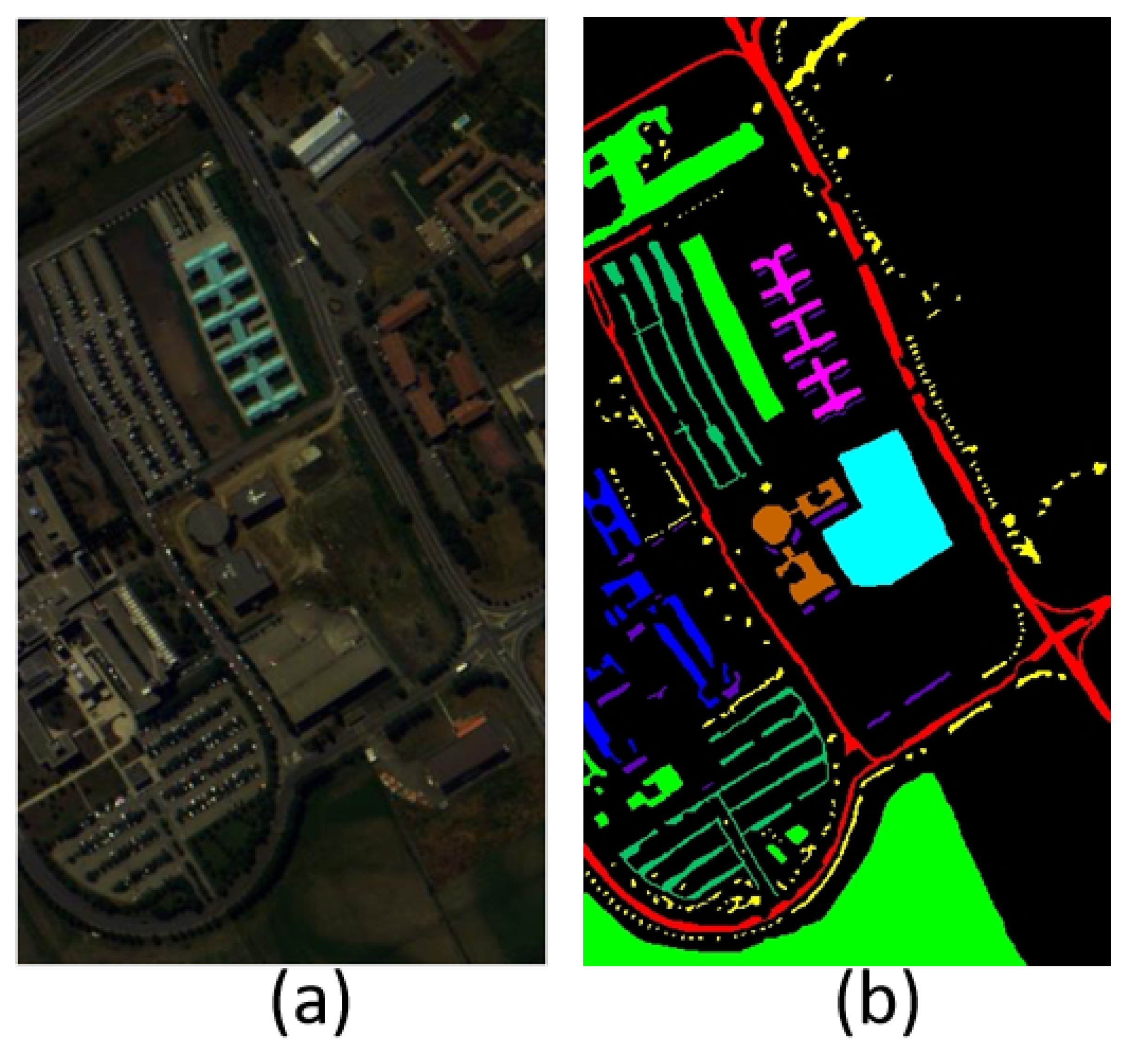
| No. | Class Name | Training | Testing | Total |
|---|---|---|---|---|
| 1 | Asphalt | 332 | 6299 | 6631 |
| 2 | Meadows | 932 | 17,717 | 18,649 |
| 3 | Gravel | 105 | 1994 | 2099 |
| 4 | Trees | 153 | 2911 | 3064 |
| 5 | Metal sheets | 67 | 1278 | 1345 |
| 6 | Bare soil | 251 | 4778 | 5029 |
| 7 | Bitumen | 67 | 1263 | 1330 |
| 8 | Bricks | 184 | 3498 | 3682 |
| 9 | Shadows | 47 | 900 | 947 |
| Total | 2138 | 40,638 | 42,776 |
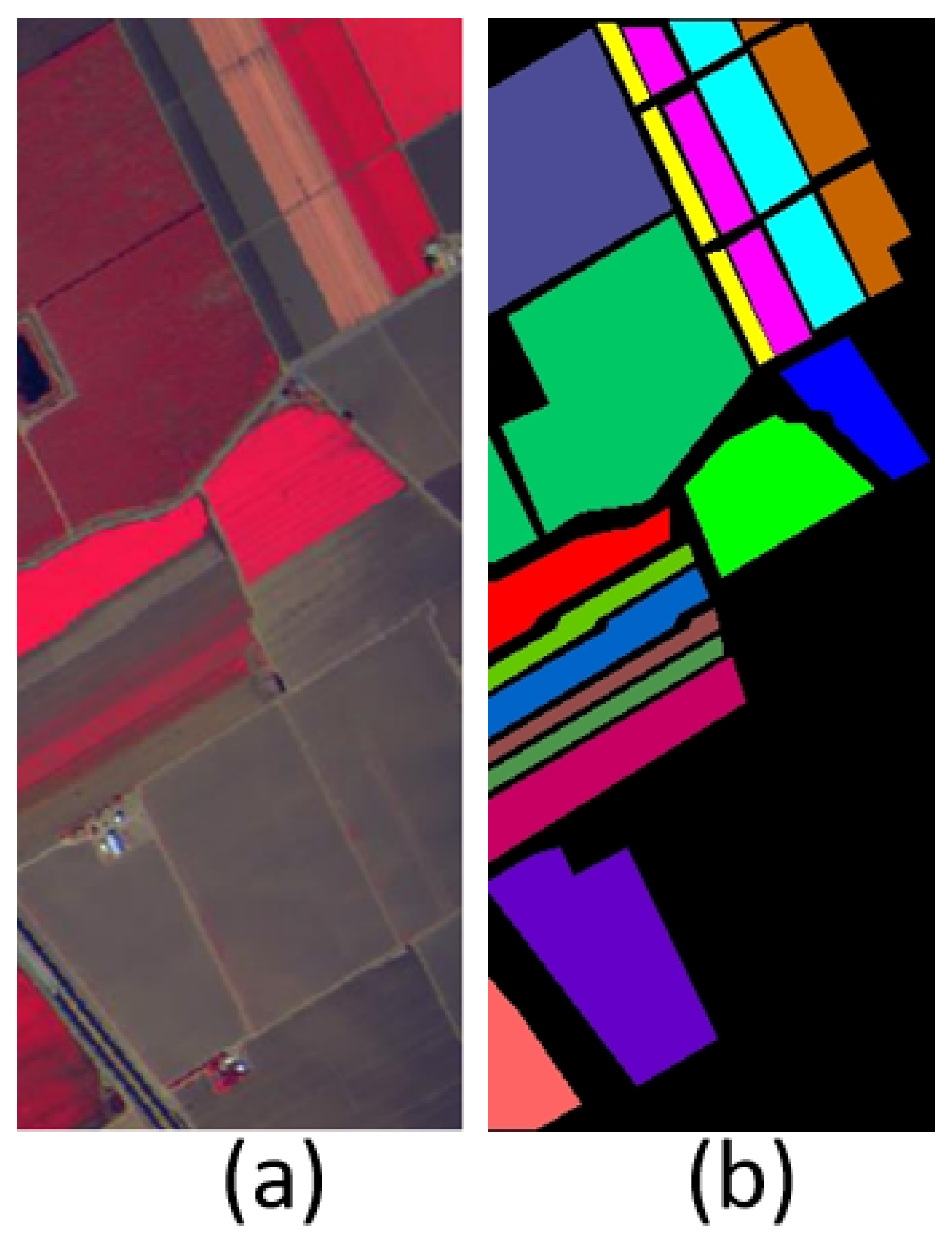
| No. | Class Name | Training | Testing | Total |
|---|---|---|---|---|
| 1 | Broccoli green weeds 1 | 10 | 1999 | 2009 |
| 2 | Broccoli green weeds 2 | 19 | 3707 | 3726 |
| 3 | Fallow | 10 | 1966 | 1976 |
| 4 | Fallow rough plow | 7 | 1387 | 1394 |
| 5 | Fallow smooth | 13 | 2665 | 2678 |
| 6 | Stubble | 20 | 3939 | 3959 |
| 7 | Celery | 18 | 3561 | 3579 |
| 8 | Grapes untrained | 56 | 11,215 | 11,271 |
| 9 | Soil vineyard develop | 31 | 6172 | 6203 |
| 10 | Corn senescence green | 16 | 3262 | 3278 |
| 11 | Lettuce romaine 4wk | 5 | 1063 | 1068 |
| 12 | Lettuce romaine 5wk | 10 | 1917 | 1927 |
| 13 | Lettuce romaine 6wk | 5 | 911 | 916 |
| 14 | Lettuce romaine 7wk | 5 | 1065 | 1070 |
| 15 | Vineyard untrained | 36 | 7232 | 7268 |
| 16 | Vineyard vertical trellis | 9 | 1798 | 1807 |
| Total | 270 | 53,859 | 54,129 |
| No. | Class Name | Training | Testing | Total |
|---|---|---|---|---|
| 1 | Healthy Grass | 125 | 1126 | 1251 |
| 2 | Stressed Grass | 125 | 1129 | 1254 |
| 3 | Synthetic Grass | 70 | 627 | 697 |
| 4 | Tree | 124 | 1120 | 1244 |
| 5 | Soil | 124 | 1118 | 1242 |
| 6 | Water | 33 | 292 | 325 |
| 7 | Residential | 127 | 1141 | 1268 |
| 8 | Commercial | 124 | 1120 | 1244 |
| 9 | Road | 125 | 1127 | 1252 |
| 10 | Highway | 123 | 1104 | 1227 |
| 11 | Railway | 123 | 1112 | 1235 |
| 12 | Parking Lot 1 | 123 | 1110 | 1233 |
| 13 | Parking Lot 2 | 47 | 422 | 469 |
| 14 | Tennis Court | 43 | 385 | 428 |
| 15 | Running Track | 66 | 594 | 660 |
| Total | 1502 | 13,527 | 15,029 |
| Class | SVM | 1D-CNN | 2D-CNN | 3D-CNN | HybridSN | SSFTT | SSFT | SMESC | MorphF | Ours |
|---|---|---|---|---|---|---|---|---|---|---|
| 1 | 70.27 | 100.00 | 100.00 | 96.97 | 86.36 | 97.22 | 90.24 | 67.44 | 84.09 | 95.12 |
| 2 | 61.82 | 71.49 | 78.99 | 78.48 | 93.92 | 95.09 | 98.94 | 96.88 | 95.96 | 98.03 |
| 3 | 38.70 | 82.76 | 90.56 | 84.57 | 89.30 | 96.65 | 98.25 | 92.01 | 97.35 | 98.27 |
| 4 | 25.40 | 73.23 | 85.09 | 85.94 | 96.39 | 93.19 | 88.73 | 85.91 | 94.76 | 94.26 |
| 5 | 91.47 | 91.08 | 94.84 | 95.10 | 97.01 | 98.33 | 94.85 | 96.71 | 93.60 | 98.46 |
| 6 | 92.98 | 97.74 | 98.61 | 98.11 | 98.72 | 99.15 | 98.98 | 98.48 | 95.98 | 98.10 |
| 7 | 77.27 | 100.00 | 69.23 | 93.33 | 100.00 | 100.00 | 60.61 | 100.00 | 100.00 | 60.00 |
| 8 | 95.55 | 94.94 | 99.20 | 98.19 | 99.12 | 99.22 | 98.44 | 98.47 | 99.21 | 99.22 |
| 9 | 37.5 | 50.00 | 90.00 | 100.00 | 100.00 | 100.00 | 100.00 | 76.19 | 99.63 | 51.52 |
| 10 | 57.97 | 77.79 | 75.77 | 83.54 | 91.32 | 91.45 | 95.33 | 92.60 | 98.51 | 99.50 |
| 11 | 73.49 | 81.05 | 86.96 | 84.72 | 94.52 | 97.45 | 99.23 | 98.46 | 98.27 | 99.28 |
| 12 | 31.58 | 72.60 | 79.86 | 81.17 | 87.42 | 95.57 | 94.92 | 89.47 | 95.54 | 95.62 |
| 13 | 90.85 | 98.18 | 96.93 | 100.00 | 98.77 | 100.00 | 100.00 | 100.00 | 100.00 | 96.69 |
| 14 | 94.07 | 95.02 | 95.31 | 95.59 | 99.06 | 99.00 | 99.80 | 99.40 | 98.92 | 99.35 |
| 15 | 41.56 | 78.01 | 82.69 | 85.17 | 90.93 | 91.12 | 96.86 | 92.40 | 98.09 | 97.89 |
| 16 | 81.33 | 94.37 | 88.46 | 96.10 | 92.41 | 97.33 | 87.14 | 92.50 | 92.96 | 92.41 |
| OA (%) | 68.99 | 83.32 | 87.41 | 87.43 | 94.47 | 96.71 | 97.67 | 95.85 | 97.20 | 98.03 |
| AA (%) | 66.36 | 72.58 | 83.87 | 82.55 | 92.89 | 95.83 | 96.68 | 93.87 | 97.29 | 97.95 |
| k × 100 | 64.34 | 80.91 | 85.62 | 86.62 | 93.69 | 96.24 | 97.34 | 95.26 | 96.81 | 97.76 |
| F1 (%) | 58.26 | 76.61 | 85.95 | 86.43 | 91.56 | 96.24 | 95.05 | 92.68 | 95.42 | 95.21 |
| Class | SVM | 1D-CNN | 2D-CNN | 3D-CNN | HybridSN | SSFTT | SSFT | SMESC | MorphF | Ours |
|---|---|---|---|---|---|---|---|---|---|---|
| 1 | 92.29 | 97.01 | 97.92 | 96.97 | 99.51 | 99.48 | 99.22 | 97.30 | 99.28 | 99.72 |
| 2 | 96.86 | 98.41 | 99.21 | 99.45 | 99.55 | 99.77 | 99.79 | 99.84 | 99.66 | 99.72 |
| 3 | 68.14 | 88.74 | 92.86 | 92.93 | 93.41 | 97.67 | 95.17 | 98.65 | 97.88 | 98.89 |
| 4 | 87.32 | 97.52 | 96.23 | 99.30 | 99.52 | 99.50 | 99.26 | 99.65 | 99.32 | 99.29 |
| 5 | 100.00 | 100.00 | 100.00 | 100.00 | 100.00 | 99.91 | 100.00 | 97.20 | 98.21 | 99.22 |
| 6 | 76.78 | 96.38 | 97.87 | 99.11 | 99.67 | 99.37 | 99.75 | 99.63 | 100.00 | 100.00 |
| 7 | 59.68 | 93.63 | 97.38 | 97.47 | 98.83 | 99.12 | 99.71 | 98.59 | 96.84 | 98.52 |
| 8 | 86.15 | 85.95 | 85.98 | 90.56 | 92.15 | 93.24 | 94.17 | 89.45 | 98.77 | 99.36 |
| 9 | 98.87 | 99.38 | 96.58 | 99.63 | 94.83 | 99.75 | 99.34 | 97.83 | 97.52 | 98.96 |
| OA (%) | 89.79 | 96.24 | 97.02 | 97.80 | 98.48 | 98.95 | 98.93 | 98.21 | 99.27 | 99.57 |
| AA (%) | 85.23 | 94.66 | 95.48 | 96.59 | 97.54 | 98.27 | 98.35 | 96.34 | 98.25 | 98.93 |
| k × 100 | 86.31 | 95.01 | 96.05 | 97.16 | 97.99 | 98.61 | 98.58 | 97.63 | 99.03 | 99.44 |
| F1 (%) | 88.54 | 95.11 | 96.75 | 97.80 | 97.96 | 98.43 | 98.42 | 97.74 | 98.42 | 99.10 |
| Class | SVM | 1D-CNN | 2D-CNN | 3D-CNN | HybridSN | SSFTT | SSFT | SMESC | MorphF | Ours |
|---|---|---|---|---|---|---|---|---|---|---|
| 1 | 99.60 | 98.74 | 100.00 | 100.00 | 99.10 | 84.39 | 100.00 | 99.40 | 99.95 | 98.51 |
| 2 | 96.43 | 95.69 | 99.51 | 98.18 | 100.00 | 98.46 | 99.73 | 99.32 | 99.92 | 98.03 |
| 3 | 94.64 | 99.49 | 97.48 | 99.79 | 91.62 | 100.00 | 98.47 | 89.08 | 78.97 | 92.16 |
| 4 | 92.90 | 94.19 | 87.18 | 92.58 | 94.74 | 58.81 | 89.97 | 81.79 | 79.74 | 86.95 |
| 5 | 78.12 | 94.31 | 97.53 | 84.72 | 97.97 | 87.77 | 98.74 | 94.14 | 95.55 | 97.61 |
| 6 | 99.00 | 96.33 | 99.39 | 95.24 | 99.44 | 97.07 | 99.42 | 98.66 | 99.40 | 99.46 |
| 7 | 98.00 | 99.00 | 98.97 | 99.78 | 99.57 | 98.47 | 99.92 | 99.92 | 96.19 | 99.97 |
| 8 | 68.64 | 79.14 | 77.27 | 79.88 | 78.44 | 95.67 | 89.15 | 99.43 | 94.81 | 95.00 |
| 9 | 86.03 | 99.39 | 98.57 | 99.09 | 98.69 | 100.00 | 96.29 | 98.63 | 99.78 | 100.00 |
| 10 | 96.41 | 96.12 | 98.31 | 92.73 | 98.34 | 95.06 | 98.07 | 98.29 | 83.51 | 98.50 |
| 11 | 92.79 | 94.00 | 98.20 | 92.87 | 83.33 | 99.83 | 95.14 | 89.89 | 96.70 | 92.34 |
| 12 | 90.07 | 93.72 | 88.82 | 96.52 | 92.00 | 94.94 | 91.24 | 84.90 | 99.37 | 96.69 |
| 13 | 57.54 | 49.75 | 65.30 | 82.95 | 81.61 | 85.96 | 64.78 | 85.96 | 97.57 | 100.00 |
| 14 | 87.84 | 50.70 | 73.89 | 90.47 | 98.67 | 75.97 | 91.35 | 94.94 | 97.48 | 95.75 |
| 15 | 69.64 | 73.85 | 75.77 | 79.89 | 80.53 | 98.49 | 67.19 | 95.70 | 94.59 | 96.50 |
| 16 | 99.42 | 82.55 | 97.35 | 87.25 | 98.69 | 100.00 | 100.00 | 96.06 | 97.86 | 100.00 |
| OA(%) | 82.83 | 87.59 | 89.55 | 90.02 | 90.89 | 94.73 | 90.10 | 96.42 | 94.84 | 97.05 |
| AA(%) | 83.11 | 87.61 | 90.22 | 91.20 | 92.08 | 93.41 | 93.25 | 94.69 | 95.06 | 96.52 |
| k × 100 | 82.09 | 86.18 | 88.33 | 88.86 | 89.84 | 94.13 | 90.01 | 96.08 | 94.26 | 96.72 |
| F1(%) | 80.29 | 86.86 | 91.06 | 91.47 | 94.02 | 96.24 | 93.18 | 94.56 | 94.61 | 97.02 |
| Class | SVM | 1D-CNN | 2D-CNN | 3D-CNN | HybridSN | SSFTT | SSFT | SMESC | MorphF | Ours |
|---|---|---|---|---|---|---|---|---|---|---|
| 1 | 95.90 | 97.60 | 97.59 | 98.19 | 100.00 | 96.31 | 99.06 | 100.00 | 100.00 | 99.50 |
| 2 | 98.70 | 96.66 | 96.62 | 97.85 | 99.37 | 99.39 | 99.48 | 97.27 | 98.15 | 99.30 |
| 3 | 99.99 | 99.00 | 98.63 | 100.00 | 99.33 | 100.00 | 100.00 | 96.99 | 100.00 | 100.00 |
| 4 | 96.79 | 97.99 | 98.50 | 98.00 | 99.60 | 97.66 | 98.95 | 99.16 | 95.57 | 93.79 |
| 5 | 99.30 | 97.30 | 98.00 | 99.99 | 100.00 | 99.10 | 100.00 | 97.72 | 100.00 | 98.91 |
| 6 | 99.62 | 98.19 | 98.00 | 99.00 | 99.92 | 100.00 | 100.00 | 99.32 | 99.63 | 100.00 |
| 7 | 92.01 | 96.99 | 97.65 | 98.28 | 99.97 | 96.94 | 95.79 | 100.00 | 97.50 | 97.65 |
| 8 | 79.72 | 93.77 | 97.58 | 97.30 | 99.95 | 100.00 | 95.80 | 99.79 | 98.38 | 97.82 |
| 9 | 81.44 | 90.85 | 94.93 | 95.28 | 99.98 | 95.04 | 94.36 | 100.00 | 92.89 | 96.39 |
| 10 | 80.73 | 94.16 | 95.30 | 95.13 | 99.76 | 98.30 | 95.71 | 93.21 | 98.21 | 98.30 |
| 11 | 86.44 | 95.37 | 95.81 | 98.10 | 99.90 | 99.60 | 96.60 | 92.63 | 99.24 | 99.90 |
| 12 | 74.57 | 90.16 | 97.28 | 95.96 | 97.25 | 98.88 | 96.50 | 92.92 | 99.90 | 100.00 |
| 13 | 63.20 | 93.63 | 95.44 | 97.61 | 99.76 | 98.06 | 95.18 | 100.00 | 98.70 | 100.00 |
| 14 | 99.42 | 93.20 | 98.12 | 99.99 | 99.99 | 99.99 | 100.00 | 99.53 | 100.00 | 100.00 |
| 15 | 98.11 | 99.97 | 97.25 | 95.65 | 99.97 | 98.51 | 97.10 | 99.48 | 98.94 | 99.98 |
| OA (%) | 89.30 | 95.39 | 96.51 | 97.01 | 97.37 | 98.27 | 97.43 | 97.85 | 98.21 | 98.40 |
| AA (%) | 89.73 | 94.69 | 96.25 | 97.04 | 97.23 | 97.90 | 97.65 | 96.27 | 98.22 | 98.38 |
| k × 100 | 88.43 | 95.09 | 96.39 | 97.65 | 97.24 | 98.12 | 97.22 | 97.87 | 98.07 | 98.27 |
| F1 (%) | 88.26 | 96.14 | 96.61 | 97.22 | 97.47 | 98.18 | 97.63 | 97.54 | 98.34 | 98.50 |
| Indicators | ViT + DCONV | Without FAF | with FFN | Ours |
|---|---|---|---|---|
| OA(%) | 98.25 | 99.27 | 99.13 | 99.57 |
| AA(%) | 97.32 | 98.25 | 98.09 | 98.93 |
| k × 100 | 98.00 | 99.03 | 98.84 | 99.44 |
| F1(%) | 98.29 | 98.42 | 98.38 | 99.10 |
| Class | 1 | 2 | 3 | 4 | 5 | 6 | 7 | 8 | 9 | OA(%) | AA(%) | k × 100 | F1(%) |
|---|---|---|---|---|---|---|---|---|---|---|---|---|---|
| DF end | 98.77 | 99.52 | 97.73 | 97.63 | 96.62 | 99.85 | 98.60 | 98.65 | 93.34 | 98.90 | 97.43 | 98.54 | 98.32 |
| Ours | 99.52 | 99.72 | 98.89 | 99.29 | 99.22 | 100.00 | 98.52 | 99.36 | 98.96 | 99.57 | 98.93 | 99.44 | 99.10 |
| Method | Test Time | Parameter Count |
|---|---|---|
| Ours | 48S | 3,172,003 |
| ViT+DONV | 72S | 7,936,299 |
Disclaimer/Publisher’s Note: The statements, opinions and data contained in all publications are solely those of the individual author(s) and contributor(s) and not of MDPI and/or the editor(s). MDPI and/or the editor(s) disclaim responsibility for any injury to people or property resulting from any ideas, methods, instructions or products referred to in the content. |
© 2025 by the authors. Licensee MDPI, Basel, Switzerland. This article is an open access article distributed under the terms and conditions of the Creative Commons Attribution (CC BY) license (https://creativecommons.org/licenses/by/4.0/).
Share and Cite
Pan, X.; Zang, C.; Lu, W.; Jiang, G.; Sun, Q. FSFF-Net: A Frequency-Domain Feature and Spatial-Domain Feature Fusion Network for Hyperspectral Image Classification. Electronics 2025, 14, 2234. https://doi.org/10.3390/electronics14112234
Pan X, Zang C, Lu W, Jiang G, Sun Q. FSFF-Net: A Frequency-Domain Feature and Spatial-Domain Feature Fusion Network for Hyperspectral Image Classification. Electronics. 2025; 14(11):2234. https://doi.org/10.3390/electronics14112234
Chicago/Turabian StylePan, Xinyu, Chen Zang, Wanxuan Lu, Guiyuan Jiang, and Qian Sun. 2025. "FSFF-Net: A Frequency-Domain Feature and Spatial-Domain Feature Fusion Network for Hyperspectral Image Classification" Electronics 14, no. 11: 2234. https://doi.org/10.3390/electronics14112234
APA StylePan, X., Zang, C., Lu, W., Jiang, G., & Sun, Q. (2025). FSFF-Net: A Frequency-Domain Feature and Spatial-Domain Feature Fusion Network for Hyperspectral Image Classification. Electronics, 14(11), 2234. https://doi.org/10.3390/electronics14112234