Ultra-Dense Uplink UAV Lossy Communications: Trajectory Optimization Based on Mean Field Game

Abstract

This paper investigates a multiple unmanned aerial vehicle (UAV) enabled network for supporting emergency communication services, where each drone acts as a base station (also called the drone small cell (DSC)). The novelty of this paper is that a mean field game (MFG)-based strategy is conceived for jointly controlling the three-dimensional (3D) locations of these drones to guarantee the distortion requirement of lossy communications, while considering the inter-cell interference and the flight energy consumption of drones. More explicitly, we derive the Hamilton–Jacobi–Bellman (HJB) and Fokker–Planck–Kolmogorov (FPK) equations, and propose an algorithm where both the Lax–Friedrichs scheme and the Lagrange relaxation are invoked for solving the HJB and FPK equations with 3D control vectors and state vectors. The numerical results show that the proposed algorithm can achieve a higher access rate with a similar flight energy consumption.

1. Introduction

With the rapid development of Internet-of-Things (IoT), it has brought severe challenges to the design of mobile wireless networks, mainly to provide high data rates and extremely low latency [1]. However, terrestrial base stations may not be available when destroyed by disasters, and cannot support the communication demands in emergency scenarios.

Due to the flexible maneuverability, easy deployment, low cost and miniaturization of unmanned aerial vehicle (UAV), it has been used in many emergency communication scenarios caused by disasters [2,3]. As one of the supporting technologies of sixth-generation (6G) wireless communication systems, the deployment of aerial base stations is also an efficient way to enhance wireless communication services. With the reduction in UAV cost, the scale of the UAV communication network can be significantly extended by introducing multiple UAVs to provide service [4]. UAVs can construct an aerial UAV swarm network through flexible networking, supplementing to the existing network architecture for wireless information transmission, which can realize rapid movement of the wireless network coverage area.

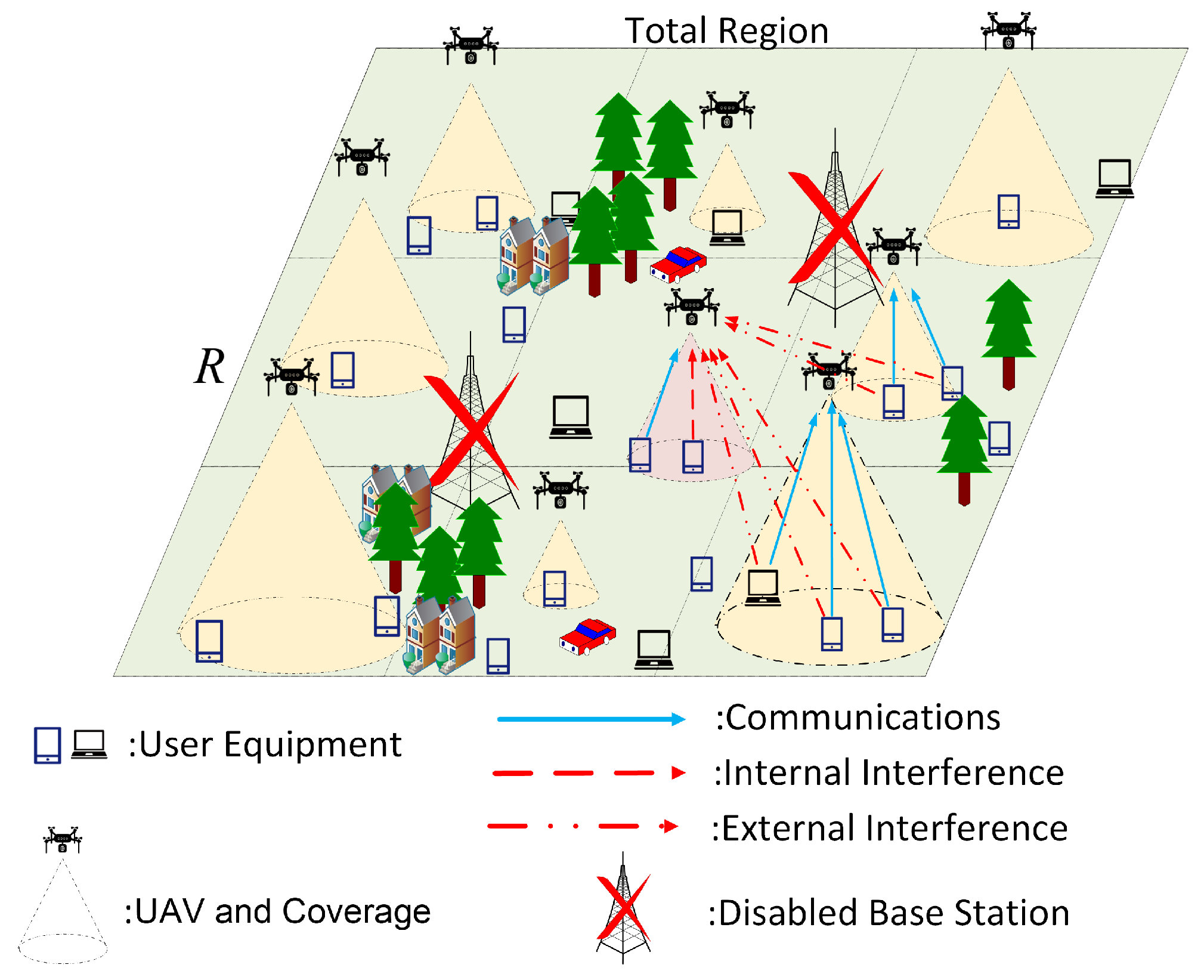
When the number of users increases in 6G networks, it is very difficult to provide satisfactory service for users [5]. Therefore, UAV communication networks will undoubtedly have to face the challenges of dense deployment scenarios [6]. A typical scenario of ultra-dense UAV communications is illustrated in Figure 1, where ground base stations are not deployed or unavailable in this area. People may encounter this situation when disasters destroy the base stations [7]. To satisfy the users’ communication demands, many UAVs carry communication devices to provide connection services to the ultra-dense users.

In the scenario where dense communication links coexist, mutual interference is a problem that network operators must face. How to achieve interference control in ultra-dense networks in a communication environment with restricted or more complicated channel conditions is still a research direction for academia and industry. By deploying UAVs at suitable positions, it can reduce the interference from the users in other cells, while maintaining a good coverage for the users in its cell.

In extreme cases, if the interference is too severe for the link to transmit information losslessly, the received information inevitably contains distortions. The conventional communication systems will discard the error-corrupted information since the lossy recovery cannot be further utilized. Nonetheless, artificial intelligence (AI)-enabled 6G networks have the capability to exploit the useful information from lossy recoveries. In task-oriented communication scenarios such as IoT [8], a certain degree of distortion is acceptable provided that the final decision is still correct. Furthermore, 6G networks may intentionally perform lossy communications, i.e., semantic communications [9,10,11,12,13] emphasize the reconstructed information having the same “meaning” rather than “bit sequences” as the original information. Thus, lossy communications have a bright future in the 6G era.

There is already some research focusing on UAV lossy communications [14,15,16]. The work in [14] proposes an optimization method for minimizing the age of information in UAV communications. The authors in [15] analyze the lossy communication performance of cooperative UAV networks. The work in [16] focuses on the adaptive communication protocol for transmitting critical video data by lossy compression. However, the scenario of these studies contains a limited number of UAVs and users. Although [17] investigates data sharing of a large-scale UAV swarm in lossy communication environments, the system objective is to reliably exchange information based on consensus algorithm instead of exploiting the lossy information. Therefore, an ultra-dense UAV network adopting lossy communications remains to be investigated. The key problem for optimizing the ultra-dense UAV network is the computing complexity of the algorithm. Especially in dynamic environment, UAVs face complex optimization constraints [18]. In ultra-dense networks, conventional optimization approaches face a huge amount of parameters to be optimized, which require incredible computing complexity. It is extremely hard to solve an optimization problem with a huge amount of parameters within a certain time. To solve this problem, mean field game (MFG) is a state-of-the-art tool which can significantly alleviate the curse of dimensionality. The so-called mean field theory is simply to average the effect of the environment on the object, by collectively processing the influence of the surrounding objects on the target, using the global average effect result to replace the effect caused by a large number of monomers. In the MFG, for a typical individual, the game with all other individuals is simplified to a game with a mean field. MFG has brought the possibility of modeling and solving such a dense network distributed by game strategies.

In recent years, MFG has gradually been used in communication scenarios [19,20]. The authors in [21] discussed the downlink interference management in dense UAVs networks using MFG theory, which modeled the interference control problem as an altitude control problem. The MFG was used to obtain the optimal altitude control strategy. In [22], a joint channel access and power control optimization problem was solved by formulating a multiple MFG for large-scale UAV networks. In [23], the authors studied a prediction-based charging policy and interference mitigation approach in wireless powered IoT networks. In these networks, it modeled the interference mitigation problem as an MFG system, where the drone powered the sensors through the appropriate path. The authors in [24] combined MFG with multi-agent deep reinforcement learning for resource allocation of UAV-assisted multi-access edge computing networks.

In summary, the numbers of UAVs and users were quite limited in many scenarios, which hardly satisfied the needs of ultra-dense scenes. Although there were some works adopting the MFG in drone communication to deal with the interference management and deployment problem, the system is designed for lossless communications, which do not fit the AI-enabled scenario in 6G.

Motivated by the aforementioned facts, this paper considers a large number of UAVs that serve multiple users in lossy communication networks, and proposes a 3D distributed dynamic flight strategy. In order to solve the problem of mutual interference minimization in the dense network of drones, we will deeply study the system optimization problem of the ultra-dense network composed of drone base stations and a large number of users. The MFG framework is used to find the best 3D position solution for drones. The main idea of the proposed algorithm is to average the interference from the mass of all users as a mean field, which significantly reduces the computing complexity for solving the optimization problem.

The main contributions of this paper are summarized as follows:

• An MFG framework for dynamic emergency communication networks: We propose an MFG framework for dynamic communication networks. The framework contains a small number of base stations and a large number of UAVs and users. Among them, the UAVs assist the base stations to provide services for the users.
• Energy consumption and location problem formulation: With the help of the proposed MFG framework, we optimize the trajectory of the UAV, and design the corresponding cost function. We formulate this problem as the problem of cost minimization, but the constraints of energy consumption and penalty must be considered.
• Constructing a robust MFG: Considering the time-varying problem of the channel, a robust mean field framework is designed to solve the trajectory optimization problem.
• Equilibrium solution of MFG: We obtain the equilibrium solution for ultra-dense uplink UAV lossy communications by alternately solving the Hamilton-Jacobi-Bellman (HJB) and Fokker-Planck-Kolmogorov (FPK) functions of MFG.

The rest of the paper is organized as follows. In Section 2, we introduce the system model and the related assumptions including the application scenarios, the channel model, the flight energy model as well as the cost function. In Section 3, the stochastic differential game and the MFG system framework are presented. In Section 4, the presented framework is derived and the iteration equations of UAV control and state are obtained. The simulation results and analyses are shown in Section 5. The conclusions are drawn in Section 6.

2. System Model

In this section, we introduce the system model of ultra-dense uplink UAV communications. Section 2.1 mathematically describes the basic scenario considered in this paper. Section 2.2 characterizes the channel model for UAV communications. Section 2.3 presents the cost function of each UAV based on the user interference and the flight energy consumption.

2.1. Basic Scenario

We consider the basic scenario illustrated in Figure 1, where the users stay in a large square region with a side length of R. To formulate the optimization problem, we make the following assumptions.

(1) The locations of the users are assumed to be independently and randomly distributed according to the Poisson point process (PPP) [25].

(2) We assume that the UAVs follow a uniform distribution in the horizontal plane, while all of the UAVs are at the same altitude. The density of users is denoted as $\mu$, and hence, the number of users can be expressed as $Q=\mu A$, where A is the area of the whole region. Moreover, the set of users is denoted as $\mathbb{Q}$.

(3) We further assume that the positions of users are constant or changing slowly during the service time $[0,T]$. Thus, the number of users in the responsible area of each UAV remains constant, and each UAV only serves the users within its responsible area.

In the considered scenario, N UAVs form a set $\mathbb{N}$ and share the same time-frequency channel for receiving uplink data from the users assigned to them. The transmit power is denoted as $P_t$, and the users request access continuously during the time interval. Under this circumstance, we have to consider the interference from other users when optimizing the UAV positions.

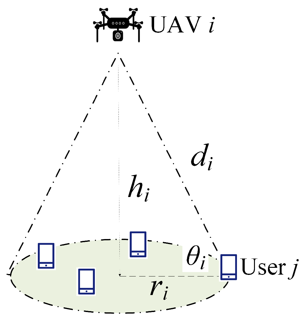
Figure 2 depicts the cell served by a UAV $i\in \mathbb{N}$. If we can guarantee the access quality of the farthest user, the access quality can also be satisfied for the other users. Without loss of generality, we assume that the user j is the farthest user in the cell. Therefore, the user j is located at the boundary of the optimal coverage area of the UAV i. The UAV i is located at the attitude $h_i$, and the radius of the coverage area is $r_i$. For simplicity, we neglect the altitude of the user and the antenna heights. Then, the distance between the UAV i and the boundary of the coverage area is $d_i=\sqrt{r_i^2+h_i^2}$, and the corresponding elevation angle is ${\theta }_i=arctan(h_i/r_i)$. Furthermore, we denote the range of the UAV flight altitude and the maximum UAV speed as $\tilde{H}=[h_{min},h_{max}]$ and $v_{max}$, respectively.

2.2. Channel Model

In this paper, the air-to-ground (A2G) channel is assumed to follow the probabilistic line-of-sight (LoS) model, where the channels between the UAVs and the users are of either the LoS or of the non-line-of-sight (NLoS) nature and their occurrence probabilities are determined by the elevation angle of the transmission link [26]. Moreover, the multiple reflected signals which cause the multi-path fading [27] are also taken into consideration.

The path-loss between the UAV i and a user k for LoS and NLoS links is denoted as $P{L}_{\mathrm{LoS},ik}$ and $P{L}_{\mathrm{NLoS},ik}$, respectively. The path-loss in dB can be expressed by [26]

$$\begin{array}{cc}\hfill P{L}_{\mathrm{LoS},ik}^{\mathrm{dB}}& =20log\left({\displaystyle \frac{4\pi f_c{d}_{ik}}{c}}\right)+{\zeta }_{\mathrm{LoS}},\hfill \end{array}$$

(1)

$$\begin{array}{cc}\hfill P{L}_{\mathrm{NLoS},ik}^{\mathrm{dB}}& =20log\left({\displaystyle \frac{4\pi f_c{d}_{ik}}{c}}\right)+{\zeta }_{\mathrm{NLoS}},\hfill \end{array}$$

(2)

where $d_{ik}$ is the distance between the UAV i and the user k. ${\zeta }_{\mathrm{LoS}}$ and ${\zeta }_{\mathrm{NLoS}}$ represent the free space propagation loss of LoS and NLoS links, respectively, which depends on the environmental conditions. $f_c$ represents the carrier frequency, and c stands for the speed of light. Moreover, the probability of LoS links is given by [27]

$$P_{\mathrm{LoS},ik}={\displaystyle \frac{1}{1+\alpha exp\left[-\beta \left({\theta }_{ik}-\alpha \right)\right]}},$$

(3)

where $\alpha$ and $\beta$ are the constants which depend on the environment, the density and height of buildings, and the elevation angle. ${\theta }_{ik}$ is the elevation angle from the user k to the UAV i. Hence, the probability of NLoS links is $P_{\mathrm{NLoS},ik}=1-P_{\mathrm{LoS},ik}$. Then, the path-loss function can be represented as

$$P{L}_{ik}^{\mathrm{dB}}=P_{\mathrm{LoS},ik}·P{L}_{\mathrm{LoS},ik}^{\mathrm{dB}}+P_{\mathrm{NLoS},ik}·P{L}_{\mathrm{NLoS},ik}^{\mathrm{dB}}.$$

(4)

By combining (1)–(4), the path-loss function can be rewritten as

$$\begin{array}{cc}\hfill P{L}_{ik}^{\mathrm{dB}}& ={\displaystyle \frac{{\zeta }_{\mathrm{LoS}}-{\zeta }_{\mathrm{NLoS}}}{1+\alpha \exp \left[-\beta \left({\theta }_{ik}-\alpha \right)\right]}}+20log\left({\displaystyle \frac{4\pi f_c{d}_{ik}}{c}}\right)+{\zeta }_{\mathrm{NLoS}},\hfill \end{array}$$

(5)

which is a function of ${\theta }_{ik}$ and $d_{ik}$. Specifically, for the user located at the boundary of the coverage area, the optimal angle ${\theta }_{\mathrm{opt}}$ equals $20.{34}^{\circ }$, $42.{44}^{\circ }$, $54.{62}^{\circ }$, and $75.{52}^{\circ }$ for the suburban, urban, dense urban and high-rise urban environments, respectively [28]. Therefore, if the value of the path-loss is given, the optimal UAV attitude and coverage radius pair $(h,r)$ can be obtained, and vice versa. Since MFG averages the mass of users’ interference, including the small-scale fading, this paper simplifies the small-scale fading by utilizing MFG.

2.3. Cost Function

For achieving higher energy efficiency while guaranteeing successful access for each user, the UAV should adjust its position jointly based on the user interference and its flight energy consumption.

The quality of user access is characterized by the distortion of the recovered information. According to the rate-distortion theory [29], the minimum rate for a Bern(0.5) source to satisfy the distortion requirement $D_i$ for the i-th UAV is given by

$$\begin{array}{c}\hfill R_i\left(D_i\right)=1-H_b\left(D_i\right),\end{array}$$

(6)

where $H_b\left(D_i\right)=-D_i{log}_2{D}_i-(1-D_i){log}_2(1-D_i)$ denotes the binary entropy function.

Based on Shannon’s lossy source-channel separation theorem, the rate is constrained by the signal-to-interference-plus-noise ratio (SINR) of the received signals as

$$\begin{array}{c}\hfill R_i\left(D_i\right)\le {\displaystyle \frac{C\left({\gamma }_i\right)}{R_{c,i}}},\end{array}$$

(7)

where $R_{c,i}$ is the end-to-end coding rate, ${\gamma }_i$ represents the SINR of the received signals, and $C\left({\gamma }_i\right)={log}_2(1+{\gamma }_i)$ denotes the channel capacity with two-dimensional signalling. Therefore, the required SINR threshold ${\gamma }_{th,i}$ can be obtained as

$$\begin{array}{c}\hfill {\gamma }_{th,i}=C^{-1}\left[R_{c,i}{R}_i\left(D_i\right)\right],\end{array}$$

(8)

with $C^{-1}(·)$ denoting the inverse function of $C(·)$. For simplicity, this paper considers the case that all distortion requirements are the same, and hence, the SINR thresholds are also the same for all links, i.e., ${\gamma }_{th,i}={\gamma }_{th}$.

At the moment t, the external interference $I_{\mathrm{out},i}\left(t\right)$ for the UAV i is caused by those users assigned to other UAVs, which can be formulated as

$$I_{\mathrm{out},i}\left(t\right)=\sum _{k\in \mathbb{Q}\setminus {\mathbb{Q}}_{\mathrm{in},i}}{P}_t{G}_{ik}\left(t\right),$$

(9)

where ${\mathbb{Q}}_{\mathrm{in},i}$ stands for the set of internal users served by the UAV i. $\mathbb{Q}\setminus {\mathbb{Q}}_{\mathrm{in},i}$ denotes the complement set of ${\mathbb{Q}}_{\mathrm{in},i}$ in $\mathbb{Q}$. $G_{ik}\left(t\right)$ represents the geometric gain, which is given by

$$\begin{array}{c}\hfill G_{ik}\left(t\right)={10}^{-P{L}_{ik}^{\mathrm{dB}}\left(t\right)/10}.\end{array}$$

(10)

For the internal user j located at the boundary of the coverage area, the internal interference $I_{\mathrm{in},i}\left(t\right)$ from the other users in the responsible area of the UAV i is

$$I_{\mathrm{in},i}\left(t\right)=\sum _{k\in {\mathbb{Q}}_{\mathrm{in},i}\setminus j}{P}_t{G}_{ik}\left(t\right).$$

(11)

Consequently, the SINR from the farthest internal user to the UAV i is readily given by

$${\gamma }_i\left(t\right)={\displaystyle \frac{P_t{G}_i\left(t\right)}{a_{\mathrm{in}}{I}_{\mathrm{in},i}\left(t\right)+a_{\mathrm{out}}{I}_{\mathrm{out},i}\left(t\right)+{\delta }^2}},$$

(12)

where ${\delta }^2$ is the power of the Gaussian white noise. $G_i\left(t\right)$ is the geometric gain from the boundary of the coverage area to the UAV i. $a_{\mathrm{in}}$ and $a_{\mathrm{out}}$ are the weights distinguishing the internal and external interference, respectively.

By minimizing the gap between the required SINR threshold ${\gamma }_{th}$ and the SINR ${\gamma }_i\left(t\right)$ of the signal received from the farthest internal user, the energy efficiency is optimized while guaranteeing the quality of user access.

Meanwhile, it is necessary to consider the flight energy consumption when planning the optimal UAV trajectory. The accumulative flight energy consumption of the UAV i at time t is given by [30]

$$\begin{array}{cc}\hfill E_{\mathrm{f},i}\left(t\right)& ={\mathcal{D}}_i\left(t\right)\left[P_{\mathrm{I}}{\left(\sqrt{1+{\displaystyle \frac{V_{\mathrm{f}}^4}{4V_0^4}}}-{\displaystyle \frac{V_{\mathrm{f}}^2}{2V_0^4}}\right)}^{{\displaystyle \frac{1}{2}}}+P_{\mathrm{B}}\left(1+{\displaystyle \frac{3V_{\mathrm{f}}^2}{V_{\mathrm{tip}}^2}}\right)+{\displaystyle \frac{1}{2}}{d}_{\mathrm{f}}\rho \eta A_{\mathrm{f}}{V}_{\mathrm{f}}^3\right],\hfill \end{array}$$

(13)

where ${\mathcal{D}}_i\left(t\right)$ stands for the flight distances. $V_0$, $V_{\mathrm{tip}}$, and $V_{\mathrm{f}}$ represent the rotor induced speed when hovering, the speed of the blade tip, and the flight speed of the UAV, respectively. $\eta$ and $\rho$ are the rotor solidity and the air density. $d_{\mathrm{f}}$ and $A_{\mathrm{f}}$ represent the fuselage drag ratio and the total area of rotary wing, respectively. The constant parameters $P_{\mathrm{I}}$ and $P_{\mathrm{B}}$ denote the induced power and the blade profile power, respectively. For simplicity, we assume that each time unit is short enough, and hence, the acceleration of UAV is neglected, which means $V_{\mathrm{f}}$ is a constant.

For enhancing the energy efficiency, the optimization problem can be formulated as

$$\begin{array}{cc}\hfill \mathbf{P}\mathbf{1}:& min{E}_{\mathrm{f},i}\left(t\right)\hfill \end{array}$$

(14)

$$\begin{array}{cc}\hfill & \mathrm{s}.\mathrm{t}.{\gamma }_i\left(t\right)\ge {\gamma }_{th}.\hfill \end{array}$$

(15)

The challenge for solving $\mathbf{P}\mathbf{1}$ is that the received power in the target and the interference to others are coupled. Increasing the received power and SINR of one UAV results in the SINR reduction of other UAVs. To solve the problem, $\mathbf{P}\mathbf{1}$ is transformed to a problem of minimizing the cost of the system, i.e.,

$$\begin{array}{cc}\hfill \mathbf{P}\mathbf{2}:& min{w}_1{\left[{\gamma }_i\left(t\right)-{\gamma }_{th}\right]}^2+w_2{E}_{\mathrm{f},i}\left(t\right),\hfill \end{array}$$

(16)

where $w_1$ and $w_2$ are the weight coefficients for the quality of user access and the energy consumption, respectively.

Moreover, two punishment functions are formulated to balance the locations between the UAV and the mass consisting of all users. One of the punishment functions is to restrain the overlap and the energy consumption caused by the height variation, which is expressed as

$${\mathcal{P}}_{i\left(1\right)}\left(t\right)={\left(A_{C,i}\left(t\right)-{\displaystyle \frac{A}{N}}\right)}^2,$$

(17)

where $A_{C,i}\left(t\right)$ is the coverage area of UAV i at time t. Clearly, $A_{C,i}\left(t\right)=\pi ·r_i^2\left(t\right)$. Another punishment function is caused by the horizontal movement of the UAV. In order to satisfy the SINR requirement ${\gamma }_i\left(t\right)\ge {\gamma }_{th}$, the UAV i will try to increase the distance from the mass. Therefore, this penalty term ${\mathcal{P}}_{i\left(2\right)}\left(t\right)=D_i\left(t\right)$ is utilized to restrain the drop-out of the mass, where $D_i\left(t\right)$ represents the distance between the UAV i and the mass at time t. Finally, the cost function of the UAV i is given by

$$\begin{array}{cc}\hfill {\mathcal{C}}_i\left(t\right)& =w_1{\left[{\gamma }_i\left(t\right)-{\gamma }_{th}\right]}^2+w_2{E}_{\mathrm{f},i}\left(t\right)+{\kappa }_1{\mathcal{P}}_{i\left(1\right)}\left(t\right)+{\kappa }_2{\mathcal{P}}_{i\left(2\right)}\left(t\right),\hfill \end{array}$$

(18)

where ${\kappa }_1$ and ${\kappa }_2$ are the coefficients of two punishment terms. The optimization problem is rewritten as

$$\begin{array}{cc}\hfill \mathbf{P}\mathbf{3}:& min{\mathcal{C}}_i\left(t\right).\hfill \end{array}$$

(19)

3. MFG for Trajectory Optimization

In this section, we establish the MFG framework of trajectory optimization for ultra-dense uplink UAV communications. To begin with, the control set and the state set of the UAVs are described in detail in Section 3.1. Then, to address a large number of distributed control of the UAVs, the MFG framework is proposed in Section 3.2.

3.1. Basic Elements in Differential Game

The problem of trajectory optimization for multiple UAV communications can be modeled as a differential game. In this game, we define the control set of the UAV i as ${\mathbb{U}}_i$, which is the set of possible 3D motion velocity vectors. The velocity vector of the UAV i at time t is given by $u_i\left(t\right)=\left\{x_i\left(t\right),y_i\left(t\right),z_i\left(t\right)\right\}\in {\mathbb{U}}_i$, where $x_i\left(t\right)$, $y_i\left(t\right)$ and $z_i\left(t\right)$ represent the velocity vector in transverse, longitudinal and vertical directions, respectively. The state set of the UAV i is formulated as ${\mathbb{S}}_i$, which is the set of 3D positions. Then, the state of the UAV i at time t is expressed as $s_i\left(t\right)=\{X_i\left(t\right),Y_i\left(t\right),h_i\left(t\right)\}$. Based on the control and state mentioned above, the position evolution of the UAV i can be written as

$$\begin{array}{c}\hfill \mathrm{d}{s}_i\left(t\right)=u_i\left(t\right)\mathrm{d}t+\sigma \mathrm{d}W\left(t\right),\end{array}$$

(20)

where $\sigma$ and $W\left(t\right)$ are the volatility and the Brownian motion, respectively. The Brownian motion $W\left(t\right)$ is a random 3D motion, which can be expressed as $W\left(t\right)=\{W_x\left(t\right),W_y\left(t\right),W_z\left(t\right)\}$. Clearly, from (20), we have

$$\begin{array}{cc}\hfill \mathrm{d}{X}_i\left(t\right)& =x_i\left(t\right)\mathrm{d}t+\sigma \mathrm{d}{W}_x\left(t\right),\hfill \end{array}$$

(21)

$$\begin{array}{cc}\hfill \mathrm{d}{Y}_i\left(t\right)& =y_i\left(t\right)\mathrm{d}t+\sigma \mathrm{d}{W}_y\left(t\right),\hfill \end{array}$$

(22)

$$\begin{array}{cc}\hfill \mathrm{d}{h}_i\left(t\right)& =z_i\left(t\right)\mathrm{d}t+\sigma \mathrm{d}{W}_z\left(t\right).\hfill \end{array}$$

(23)

In order to optimize the UAV trajectory, the problem can be equivalently solved by minimizing the cost function. Specifically, during the time interval $[0,T]$, the UAV i obtains the optimal control strategy $u_i^{*}\left(t\right)$ by minimizing the cost function (18), i.e.,

$$u_i^{*}\left(t\right)=\arg \underset{u_i\left(t\right)\in {\mathbb{U}}_i}{\min }\mathrm{E}\left[{\int }_0^T{\mathcal{C}}_i\left(t\right)dt+{\mathcal{C}}_i\left(T\right)\right].$$

(24)

Then, the value function $v_i\left(t\right)$ indicating the minimum cost of the given dynamic system is defined as

$$\begin{array}{cc}\hfill v_i(t,s_i\left(t\right))& =\underset{u_i\left(t\right)\in {\mathbb{U}}_i}{\min }\mathrm{E}\left[{\int }_t^T{\mathcal{C}}_i\left(t\right)dt+v_i(T,s_i\left(T\right))\right],t\in [0,T],\hfill \end{array}$$

(25)

where $v_i(T,s_i\left(T\right))$ represents the value function at time $t=T$. This value function should satisfy a partial differential equation, called the HJB equation [31], which is defined as

$$\begin{array}{cc}\hfill & \underset{u_i\left(t\right)\in {\mathbb{U}}_i}{min}\left[{\mathcal{C}}_i(t,u_i\left(t\right),s_i\left(t\right))-u_i\left(t\right)·{\displaystyle \frac{\partial v_i(t,s\left(t\right))}{\partial s}}\right]+{\displaystyle \frac{\partial v_i(t,s\left(t\right))}{\partial t}}=0,\hfill \end{array}$$

(26)

where the first term is known as the Hamiltonian, i.e.,

$$\begin{array}{cc}\hfill H\left(\mathcal{C},{\displaystyle \frac{\partial v_i(t,s_i\left(t\right))}{\partial s}}\right)& =\underset{u_i\left(t\right)\in {\mathbb{U}}_i}{min}\left[{\mathcal{C}}_i(t,u_i\left(t\right),s_i\left(t\right))-u_i\left(t\right)·{\displaystyle \frac{\partial v_i(t,s_i\left(t\right))}{\partial s}}\right]\hfill \\ \hfill & =\underset{u_i\left(t\right)\in {\mathbb{U}}_i}{min}[w_1{\left({\gamma }_i\left(t\right)-{\gamma }_{th}\right)}^2+w_2{E}_{\mathrm{f},i}\left(t\right)+{\kappa }_1{\mathcal{P}}_{i\left(1\right)}\left(t\right)\hfill \\ \hfill & +{\kappa }_2{\mathcal{P}}_{i\left(2\right)}\left(t\right)-u_i\left(t\right)·{\displaystyle \frac{\partial v_i(t,s_i\left(t\right))}{\partial s}}].\hfill \end{array}$$

(27)

Proof. 

Refer to Appendix A.    □

All order derivatives of the Hamiltonian $H\left(\mathcal{C},{\displaystyle \frac{\partial v_i(t,s_i\left(t\right))}{\partial s}}\right)$ exist due to the continuity of the cost function ${\mathcal{C}}_i\left(t\right)$. Therefore, the Hamiltonian $H\left(\mathcal{C},{\displaystyle \frac{\partial v_i(t,s_i\left(t\right))}{\partial s}}\right)$ is smooth, which means that a solution to the HJB Equation (26) exists. By solving the HJB equation, we can obtain the equilibrium solution of the differential game. Consequently, the existence of Nash equilibrium for the differential game is proved.

Due to a large number of UAVs, N partial differential equations need to be solved to obtain equilibrium for N players’ game, which is unrealistic. Therefore, the MFG framework is proposed to significantly simplify the system based on the mean field term and two sets of equations.

3.2. MFG Framework

Hereafter, we introduce the MFG framework for the movement of N UAVs, which is composed of two coupled HJB and FPK [32] equations. We can obtain the optimal control of each UAV by solving the backward equation (HJB equation), while the forward equation (FPK equation) describes the evolution of the mass, which represents the evolution of the mean field.

In the MFG framework, each UAV would take rational control individually to minimize the cost function. Given a sufficiently large N, the continuity of the mean field can be guaranteed. Furthermore, the players just need to interact with the mean field, and the permutation of the states among the players would not affect the outcome of the game. The mean field term is defined as $m(t,s)$, which is the state probability distribution of N UAVs as follows.

Definition 1.

With the given state $s_i\left(t\right)=\left\{X_i\left(t\right),Y_i\left(t\right),h_i\left(t\right)\right\}$, the mean field term, called the normalized density function, is given by

$$m(t,s)=\underset{N\to \infty }{lim}{\displaystyle \frac{1}{N}}\sum _{i=1}^N{\mathbb{1}}_{\{s_i\left(t\right)=s\}},$$

(28)

where $\mathbb{1}$ means that it will return 1 when $s_i\left(t\right)=s$, and otherwise, it returns 0.

To implement the MFG framework, it is necessary to transform the cost function of the general differential game to that of the MFG. Now, we derive the cost function under the MFG framework corresponding to (18). The first term in (18) represents the satisfaction of user access, which is constituted of the difference between the SINR of received signals and the SINR threshold. Thus, the SINR in (12) can be rewritten for MFG as:

$${\overline{\gamma }}_i\left(t\right)={\displaystyle \frac{P_t{G}_i\left(t\right)}{a_{\mathrm{in}}{\overline{I}}_{\mathrm{in},i}\left(t\right)+a_{\mathrm{out}}{\overline{I}}_{\mathrm{out},i}\left(t\right)+{\delta }^2}},$$

(29)

where the ${\overline{I}}_{\mathrm{in},i}\left(t\right)$ and ${\overline{I}}_{\mathrm{out},i}\left(t\right)$ are the mean field interferences, which can be expressed as:

$$\begin{array}{cc}\hfill {\overline{I}}_{\mathrm{in},i}\left(t\right)& =P_t{\int }_{\mathbb{S}}m(t,s){\overline{G}}_{\mathrm{in},i}\left(t\right)\mathrm{d}s,\hfill \end{array}$$

(30)

$$\begin{array}{cc}\hfill {\overline{I}}_{\mathrm{out},i}\left(t\right)& =P_t{\int }_{\mathbb{S}}m(t,s){\overline{G}}_{\mathrm{out},i}\left(t\right)\mathrm{d}s.\hfill \end{array}$$

(31)

${\overline{G}}_{\mathrm{in},i}\left(t\right)$ and ${\overline{G}}_{\mathrm{out},i}\left(t\right)$ are the mean field geometric gains of the internal users and the external users, respectively.

Then, by substituting (29) into (18), the mean field cost function can be defined as

$$\begin{array}{cc}\hfill {\overline{\mathcal{C}}}_i(t,m(t,s))& =w_1{\left[{\overline{\gamma }}_i\left(t\right)-{\gamma }_{th}\right]}^2+w_2{E}_{\mathrm{f},i}\left(t\right)+{\kappa }_1{\mathcal{P}}_{i\left(1\right)}\left(t\right)+{\kappa }_2{\mathcal{P}}_{i\left(2\right)}\left(t\right).\hfill \end{array}$$

(32)

Based on the mean field cost function mentioned above, we can define the HJB equation of MFG as follows.

Definition 2.

The HJB equation of MFG can be expressed as

$${\displaystyle \frac{\partial v(t,s)}{\partial t}}+\underset{u(t,s)\in \mathbb{U}}{min}\left[\overline{\mathcal{C}}(t,m(t,s))-u\left(t\right)·{\displaystyle \frac{\partial v(t,s)}{\partial s}}\right]=0.$$

(33)

Moreover, the Hamiltonian can be expressed as

$$\begin{array}{c}\hfill H\left(\overline{\mathcal{C}},{\displaystyle \frac{\partial v(t,s)}{\partial s}}\right)=\underset{u(t,s)\in \mathbb{U}}{min}\left[\overline{\mathcal{C}}(t,m(t,s))-u\left(t\right)·{\displaystyle \frac{\partial v(t,s)}{\partial s}}\right].\end{array}$$

(34)

The HJB equation is solved inversely in the time domain from $t=T$ to $t=0$, which can calculate the optimal control of each UAV. Then, we derive the FPK equation of the mean field framework defined above as:

$${\displaystyle \frac{\partial m(t,s)}{\partial t}}-{\displaystyle \frac{\partial }{\partial s}}\left[m(t,s)·u\left(t\right)\right]=0,$$

(35)

which describes the evolution of the mass and evolves forward with time. In this MFG framework, the HJB and FPK equations evolve interactively and finally reach the mean field equilibrium (MFE).

4. Energy-Efficient Flight Strategy

In this section, we obtain the energy-efficient flight strategy by solving the HJB and FPK Equations (33) and (35). These two equations are coupled mutually and interact with each other, which can reach the MFE by resorting to the finite difference method [33].

In this finite difference framework, the time space $[0,T]$ and the 3D vector space representing the location space, including 2D vector space in the horizontal direction $[0,X_{\max }]$, $[0,Y_{\max }]$ and vector space in the vertical direction $[0,h_{\max }]$, respectively, are discretized into $W\times X\times Y\times Z$ spaces. Then, we aim to find the optimal control policy in this four-dimensional discrete vector space including the time space and the location space. Hence, we define

$$\begin{array}{c}\hfill \Delta t:={\displaystyle \frac{T}{W}},\Delta X:={\displaystyle \frac{X_{max}}{X}},\Delta Y:={\displaystyle \frac{Y_{max}}{Y}},\Delta h:={\displaystyle \frac{h_{max}}{Z}},\end{array}$$

(36)

which represent the iteration steps of the time, the transverse vector, the longitudinal vector, and the vertical vector, respectively.

Then, we use the Lax–Friedrichs schemes to solve the FPK equation in (35). Let n denote time index, j, k and l denote location coordinate indices in the discretized grid. Therefore, we have the iterative equation of mean field term as

$$\begin{array}{cc}\hfill m_{j,k,l}^{n+1}& ={\displaystyle \frac{1}{2}}\left[\left(m_{j+1,k,l}^n+m_{j-1,k,l}^n\right)+\left(m_{j,k+1,l}^n+m_{j,k-1,l}^n\right)+\left(m_{j,k,l+1}^n+m_{j,k,l-1}^n\right)\right]\hfill \\ \hfill & -\left(\mathrm{\Xi }+\mathrm{\Psi }+\mathrm{H}\right),\hfill \end{array}$$

(37)

where $\mathrm{\Xi }$, $\mathrm{\Psi }$, and $\mathrm{H}$ are given by

$$\begin{array}{cc}\hfill \mathrm{\Xi }& ={\displaystyle \frac{\Delta t}{2\Delta X}}\left(m_{j+1,k,l}^n·x_{j+1,k,l}^n-m_{j-1,k,l}^n·x_{j-1,k,l}^n\right),\hfill \end{array}$$

(38)

$$\begin{array}{cc}\hfill \mathrm{\Psi }& ={\displaystyle \frac{\Delta t}{2\Delta Y}}\left(m_{j,k+1,l}^n·y_{j,k+1,l}^n-m_{j,k-1,l}^n·y_{j,k-1,l}^n\right),\hfill \end{array}$$

(39)

$$\begin{array}{cc}\hfill \mathrm{H}& ={\displaystyle \frac{\Delta t}{2\Delta h}}\left(m_{j,k,l+1}^n·z_{j,k,l+1}^n-m_{j,k,l-1}^n·z_{j,k,l-1}^n\right).\hfill \end{array}$$

(40)

$m_{j,k,l}^n$, $x_{j,k,l}^n$, $y_{j,k,l}^n$, and $z_{j,k,l}^n$ denote the value of the mean field, the transverse control, the longitudinal control and the vertical control, respectively.

In order to solve the HJB equation, we have to consider the constraints of the forward equation and mean field. Therefore, we use the Lagrange relaxation to solve the HJB equation. The Lagrangian $L\left(m\left(t,s\right),u\left(t,s\right),\lambda (t,s)\right)$ is defined as

$$\begin{array}{cc}\hfill & L\left(m\left(t,s\right),u\left(t,s\right),\lambda (t,s)\right)\hfill \\ \hfill & =\underset{t=0}{\overset{T}{\int }}\underset{X=0}{\overset{X_{max}}{\int }}\underset{Y=0}{\overset{Y_{max}}{\int }}\underset{h=0}{\overset{h_{max}}{\int }}\left[{\partial }_{t}m(t,s)-{\partial }_S\left(m(t,s)·u(t,s)\right)\right]·\lambda \left(t,s\right)dtdXdYdh\hfill \\ \hfill & +\mathrm{E}\left[{\int }_0^T{\overline{\mathcal{C}}}_n\left(t\right)dt+{\overline{\mathcal{C}}}_n\left(T\right)\right]\hfill \\ \hfill & =\underset{t=0}{\overset{T}{\int }}\underset{X=0}{\overset{X_{max}}{\int }}\underset{Y=0}{\overset{Y_{max}}{\int }}\underset{h=0}{\overset{h_{max}}{\int }}\left[\left[{\partial }_{t}m(t,s)-{\partial }_S\left(m(t,s)·u(t,s)\right)\right]·\lambda \left(t,s\right)+\overline{\mathcal{C}}(t,s)m(t,s)\right]dtdXdYdh,\hfill \end{array}$$

(41)

where $\lambda (t,s)$ is the Lagrange multiplier. Here, ${\partial }_S(m(t,s)·$$u(t,s))$ is defined as

$$\begin{array}{cc}\hfill {\partial }_S\left(m(t,s)·u(t,s)\right)& ={\partial }_X\left(m(t,s)·x(t,s)\right)+{\partial }_Y(m(t,s)·y(t,s))+{\partial }_h\left(m(t,s)·z(t,s)\right).\hfill \end{array}$$

(42)

We solve (41) by using the finite difference method. Similar to the previous method of solving the FPK equation, we discretize the Lagrangian as

$$\begin{array}{cc}\hfill L_{\Delta s,\Delta t}& ={\displaystyle \sum _{n=1}^{W+1}}{\displaystyle \sum _{j=1}^{X+1}}{\displaystyle \sum _{k=1}^{Y+1}}{\displaystyle \sum _{l=1}^{Z+1}}\left[{\overline{\mathcal{C}}}_{j,k,l}^n·m_{j,k,l}^n+{\lambda }_{j,k,l}^n·\mathrm{\Lambda }\right]\hfill \\ & ·\Delta X\Delta Y\Delta h\Delta t,\hfill \end{array}$$

(43)

where ${\overline{\mathcal{C}}}_{j,k,l}^n$ and ${\lambda }_{j,k,l}^n$ represent the value of the cost function and the Lagrange multiplier at time n location $(j,k,l)$ on the discretized grid, respectively. Here, $\mathrm{\Lambda }$ is given by

$$\begin{array}{cc}\hfill \mathrm{\Lambda }& ={\displaystyle \frac{1}{\Delta t}}[m_{j,k,l}^{n+1}-{\displaystyle \frac{1}{2}}(m_{j+1,k,l}^n+m_{j-1,k,l}^n+m_{j,k+1,l}^n+m_{j,k-1,l}^n+m_{j,k,l+1}^n+m_{j,k,l-1}^n)]\hfill \\ \hfill & -\left({\displaystyle \frac{\mathrm{\Xi }+\mathrm{\Psi }+\mathrm{H}}{\Delta t}}\right).\hfill \end{array}$$

(44)

In this model, the optimal decision variables include $u^{*}=\left\{x^{*},y^{*},z^{*}\right\}$, $m^{*}$ and ${\lambda }^{*}$. To begin with, we update the value of the Lagrange multiplier by calculating $\frac{\partial L_{\Delta s,\Delta t}}{\partial m_{j,k,l}^n}=0$. Therefore, we can obtain the iterative equation of variables $\lambda$ as

$$\begin{array}{cc}\hfill {\lambda }_{j,k,l}^{n-1}& ={\displaystyle \frac{1}{2}}({\lambda }_{j+1,k,l}^n+{\lambda }_{j-1,k,l}^n+{\lambda }_{j,k+1,l}^n+{\lambda }_{j,k-1,l}^n+{\lambda }_{j,k,l+1}^n+{\lambda }_{j,k,l-1}^n)\hfill \\ \hfill & +{\displaystyle \frac{\Delta t·x_{j,k,l}^n}{2\Delta X}}\left({\lambda }_{j-1,k,l}^n-{\lambda }_{j+1,k,l}^n\right)+{\displaystyle \frac{\Delta t·y_{j,k,l}^n}{2\Delta Y}}\left({\lambda }_{j,k-1,l}^n-{\lambda }_{j,k+1,l}^n\right)\hfill \\ \hfill & +{\displaystyle \frac{\Delta t·z_{j,k,l}^n}{2\Delta h}}\left({\lambda }_{j,k,l-1}^n-{\lambda }_{j,k,l+1}^n\right)-\Delta t{\overline{\mathcal{C}}}_{j,k,l}^n,\hfill \end{array}$$

(45)

where $n,j,k,l$ are arbitrary on this discretized grid. Then, we update the value of the control by calculating ${\displaystyle \frac{\partial L_{\Delta s,\Delta t}}{\partial x_{j,k,l}^n}}=0$, ${\displaystyle \frac{\partial L_{\Delta s,\Delta t}}{\partial y_{j,k,l}^n}}=0$ and ${\displaystyle \frac{\partial L_{\Delta s,\Delta t}}{\partial z_{j,k,l}^n}}=0$, respectively. Therefore, the iterative equation of control $x\left(t\right)$ can be expressed as follows:

$$\sum _{j=1}^{X+1}\sum _{k=1}^{Y+1}\sum _{l=1}^{Z+1}{m}_{j,k,l}^n{\displaystyle \frac{\partial {\overline{\mathcal{C}}}_{j,k,l}^n}{\partial x_{j,k,l}^n}}-{\displaystyle \frac{m_{j,k,l}^n}{2\Delta X}}\left({\lambda }_{j-1,k,l}^n-{\lambda }_{j+1,k,l}^n\right)=0.$$

(46)

Similarly, we can obtain the iterative equations of y and z as

$$\sum _{j=1}^{X+1}\sum _{k=1}^{Y+1}\sum _{l=1}^{Z+1}{m}_{j,k,l}^n{\displaystyle \frac{\partial {\overline{\mathcal{C}}}_{j,k,l}^n}{\partial y_{j,k,l}^n}}-{\displaystyle \frac{m_{j,k,l}^n}{2\Delta Y}}\left({\lambda }_{j,k-1,l}^n-{\lambda }_{j,k+1,l}^n\right)=0,$$

(47)

$$\sum _{j=1}^{X+1}\sum _{k=1}^{Y+1}\sum _{l=1}^{Z+1}{m}_{j,k,l}^n{\displaystyle \frac{\partial {\overline{\mathcal{C}}}_{j,k,l}^n}{\partial z_{j,k,l}^n}}-{\displaystyle \frac{m_{j,k,l}^n}{2\Delta h}}\left({\lambda }_{j,k,l-1}^n-{\lambda }_{j,k,l+1}^n\right)=0.$$

(48)

Finally, the MFE is solved by (37) and (46)–(48) iteratively until they converge. The specific iteration step is displayed in Algorithm 1.

Algorithm 1 Obtaining the MFE

1: Initialization:  2: $m_{:}^0$: initialize mean-field distribution;  3: ${\lambda }_{:}^{W+1}$: initialize Lagrangian parameters;  4: $u_{:}^{W+1}:=x_{:}^{W+1},y_{:}^{W+1},z_{:}^{W+1}$: initial control.  5: Repeat: Until the system obtains the MFE  6: Compute update for the mean-field m:  7: for $n=1:W$, $j\in 1,...,X$, $k\in 1,...,Y$, and $l\in 1,...,h$ do  8:    Update $m_{n,j,k}^{n+1}$ using (37).  9: end for 10: Compute update for the Lagrangian parameters $\lambda$: 11: for $n=W:1$, $j\in 1,...,X$, $k\in 1,...,Y$, and $l\in 1,...,h$ do 12:    Update ${\lambda }_{n,j,k}^{n-1}$ using (45). 13: end for 14: Compute update for the control u: 15: for $n=W:1$, $j\in 1,...,X$, $k\in 1,...,Y$, and $l\in 1,...,h$ do 16:    Update $x_{n,j,k}^{n-1}$ using (46). 17: end for 18: for $n=W:1$, $j\in 1,...,X$, $k\in 1,...,Y$, and $l\in 1,...,h$ do 19:    Update $y_{n,j,k}^{n-1}$ using (47). 20: end for 21: for $n=W:1$, $j\in 1,...,X$, $k\in 1,...,Y$, and $l\in 1,...,h$ do 22:    Update $z_{n,j,k}^{n-1}$ using (48). 23: end for

In Algorithm 1, we solve the FPK equation by iterating the mean field term m. During the iteration, if j equals 1 or X, we assume ${\displaystyle \frac{1}{2}}(m_{j+1,:}^n+m_{j-1,:}^n)=m_{j,:}^n$, and the term $m_{j-1,k,l}^n·x_{j-1,k,l}^n$ in (38) can be expressed as $m_{j,k,l}^n·x_{j,k,l}^n$. k, l are similar to j. On the other hand, the HJB equation can be solved by reversely iterating the Lagrange multiplier $\lambda$ and the control u. The end condition of iterations is the convergence point appearing or exceeding the number of iteration steps. We assume that the coordinates of the UAV in the area are positive. The values of control and the mean field term are positive for any time n and any state $(j,k,l)$. Therefore, the reformulated problem with the constraints mentioned above is a convex optimization problem. Meanwhile, the conditions of this algorithm (iterative equations) satisfy the necessary and sufficient conditions of the convex optimization problem. In other words, this convergence point is the MFE with the cost function $\overline{\mathcal{C}}\left(t\right)$.

5. Numerical Results

In this section, we evaluate the system performance with the main simulation parameter settings listed in

Table 1. Parameters in simulations.

Parameters	Value	Parameters	Value	Parameters	Value
$\mu$	$0.1$ Users/m2	$\alpha$	$9.6$	$\eta$	$0.05$
R	10 km	$\beta$	$0.28$	$A_{\mathrm{f}}$	$0.5$ m2
$P_t$	30 dBm	$\theta$	${80}^{\circ }$	${\zeta }_{\mathrm{LoS}}$	1 dB
${\gamma }_{th}$	10 dB	$V_{\mathrm{f}}$	30 m/s	${\zeta }_{\mathrm{NLoS}}$	20 dB
$f_c$	2 GHz	$V_{\mathrm{tip}}$	120 m/s	$a_{\mathrm{in}}$	$0.6$
c	$3\times {10}^8$ m/s	$V_0$	4 m/s	$a_{\mathrm{out}}$	$0.4$
$\rho$	$1.225$ kg/m3	$d_{\mathrm{f}}$	$0.6$	$[h_{min},h_{max}]$	$[1,2]$ km

. We assume the coordinate origin of the UAV location is located in the lower left corner of the desired area, so that the state of the UAV is positive. The side length of the large square geographical region (desired area) is set as $R=10$ km, which means the maximum value of the horizontal area $X_{max}=Y_{max}=10$ km. In this model, the minimum and the maximum altitudes of UAVs are $h_{\min }=1$ km and $h_{max}=2$ km, respectively, which ensures the complete coverage of users in each small area.

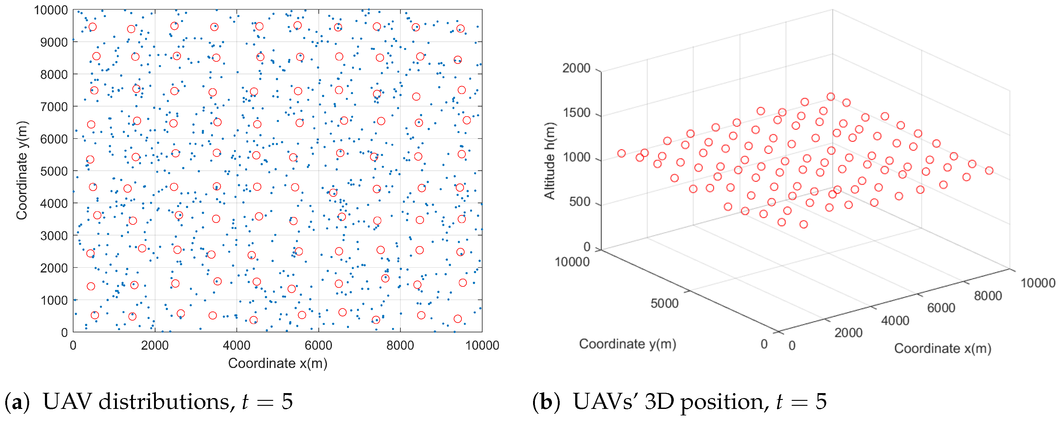
At the initial time, 100 UAVs are hovering at initial positions. The initial distributions of the UAVs and users are shown in Figure 3. The red circles represent the UAVs and the blue stars represent the users. In the horizontal direction, these 100 UAVs populate the desired area and each UAV has its responsible area, which is the small rectangle in Figure 3. The users are of random positions and numbers in each small rectangle. Meanwhile, each UAV has the same altitude $h_0$. We also illustrate the user and UAV distributions in Figure 4, where we assume that the initial altitude of users ranges from 0 to 5 m.

To illustrate the evolution of the mean field state under the control obtained by Algorithm 1 over a predefined period of time $t\in [0,T]$, we provide the distribution of the mass UAVs at different times, as shown in Figure 5. Here, T is set as 15 s. Figure 5 shows the changes in the distribution of the UAV at three times, namely, t = 5 s, 10 s, and 15 s. In Figure 5a–c, we show the 2D distribution of the UAVs (red circles) and users (blue stars) at those three moments. Meanwhile, we show the position changes of 100 UAVs in 3D space, which can be seen from Figure 5d–f. Compared with the initial time $t=0$, the 100 UAVs find the optimal locations to ensure users’ access. The users’ access status is presented in Figure 6.

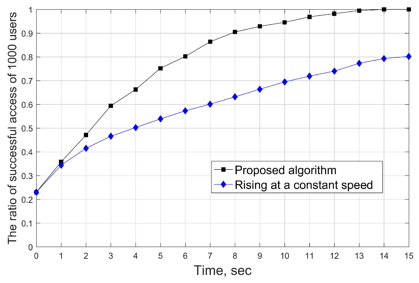
To verify the users’ access situation under these flight conditions, we show the access situation of all users in the predefined period of time $t\in [0,T]$ in Figure 6. The black curve shows the rate of successful access of all users by adopting our proposed algorithm. At the initial time, the ratio of successful access of all users is at a lower level because the altitude of UAVs is lower and the initial position is certain, which corresponds to a smaller coverage area and the incorrect position. Then, all UAVs adjust their positions with the 3D optimal control. The ratio of successful access of all users rises until they all can access. Clearly, it is seen that this ratio reaches 1 at t = 14, which means that when the system reaches equilibrium, the user’s access target will be satisfied. For comparison, we assume that all UAVs increase access ratio in the same flight mode (rising at a constant speed), as shown in Figure 6. It can be observed that the ratio of user’s access is still at $0.8$ and the growth is slow until the last time t = 15. Clearly, there is an obvious gap between the proposed algorithm and the benchmark scheme for the ratio of successful access. This is because the solution derived from the HJB equation follows the Bellman principle of optimality, which selects the optimal actions for system control.

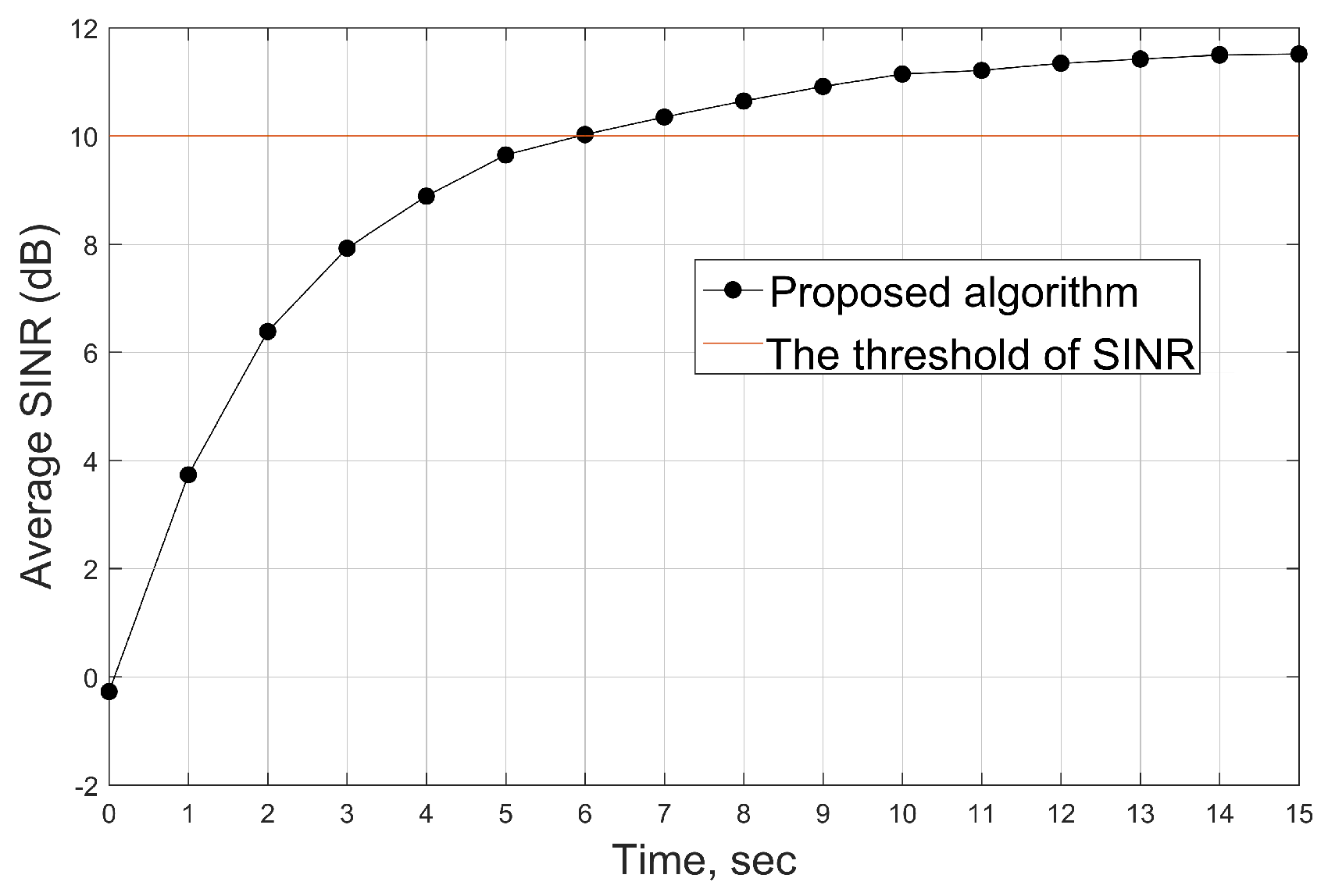
To further illustrate the user’s access rate, we show the average SINR from time 0 to T, as shown in Figure 7. The red straight line represents the threshold of SINR. At the initial time, the average SINR is low enough because there are only a few users satisfying the access requirement. It can be seen that the average SINR reaches the threshold we set above after t = 6. Corresponding to Figure 6, at t = 6, the user’s access rate reaches $0.8$, which means 20% of the users still have lower SINR, which leads to the average SINR still rising. Moreover, MFE can be achieved until the optimal position is reached because the average SINR is basically unchanged. In addition, as another important term of the cost function, the flight energy consumption will be shown in Figure 8.

In Figure 8, we present the average flight energy consumption of 100 UAVs. At the initial time, all UAVs hover at the same altitude (1000 m), and the initial energy consumption (hover energy consumption) is 60 J/s. Then, each UAV flies by adopting the optimal control, which leads to a higher average flight energy consumption at the beginning for achieving the SINR requirements. Subsequently, the average energy consumption decreases because the closer target area implies that more users are capable of reaching the threshold of SINR. The equilibrium emerges when all users arrive at the SINR threshold. At that time, each UAV keeps hovering, and the flight energy is restored to 60 J/s. The red straight line represents the average energy consumption of 100 UAVs by rising at a constant speed. The energy consumption is a constant at each time. Combining with Figure 6, when the proposed algorithm arrives at equilibrium, the total energy consumption by all UAVs is close to the energy consumption of all UAVs rising at the same speed by using the same time, but the users’ access rate is higher.

6. Conclusions

This paper has proposed a multi-UAV framework for emergency communication networks with ultra-dense ground users. In this framework, each UAV decides its own 3D flight trajectory for maximizing users’ communication qualities and the ratio of successful access under the flight energy consumption constraint. The system is modelled as an MFG, where N UAVs perform distributed controls based on their own local information. After designing the cost function and the value function of this system, we derive the HJB and FPK equations of the system. To obtain the solution, we adopt the Lax–Friedrichs scheme and the Lagrange relaxation, and demonstrate the existence of the MFE using strict proof. The numerical results show that the average SINR of all users arrives at the SINR threshold and the ratio of successful access of all users achieves 100% with the controls solved from MFG. Moreover, the comparison with the benchmark schemes verifies that the proposed algorithm has a higher access rate with a similar flight energy consumption. In the future, this work can be extended from the asymptotic convergence to a faster convergence approach, such as fixed-time convergence [34].