Abstract
To improve the robustness of intrusion detection systems constructed using deep learning models, a method based on an auxiliary adversarial training WGAN (AuxAtWGAN) is proposed from the defender’s perspective. First, one-dimensional traffic data are downscaled and processed into two-dimensional image data via a stacked autoencoder (SAE), and mixed adversarial samples are generated using the fast gradient sign method (FGSM), Projected Gradient Descent (PGD) and Carlini and Wagner (C&W) adversarial attacks. Second, the improved WGAN with an integrated perceptual network module is trained with mixed training samples composed of mixed adversarial samples and normal samples. Finally, the adversary-trained AuxAtWGAN model is attached to the original model for adversary sample detection, and the detected adversary samples are removed and input into the original model to improve the robustness of the original model. The average attack success rate of the original convolutional neural network (CNN) model against multiple adversarial samples is 75.17%, and after using AuxAtWGAN, the average attack success rate of the adversarial attacks decreases to 27.56%; moreover, the detection accuracy of the original CNN model against normal samples is still 93.57%. The experiment proves that AuxAtWGAN improves the robustness of the original model. In addition, validation experiments are conducted by attaching the AuxAtWGAN model to the Long Short-Term Memory Network (LSTM) and Residual Network34 (ResNet) models, which prove that the proposed method has high generalization performance.
1. Introduction
With the acceleration of the informationization process and the widespread popularity of internet applications, the complexity and scale of network attacks have increased, and traditional means of security protection have had difficulty coping with increasing security threats. An intrusion detection system (IDS), as a core technology in the network security defense system, can analyze network traffic in real time, detect abnormal behaviors, and provide early warning of potential attacks [1]. In recent decades, IDSs based on traditional machine learning techniques have played an important role to some extent. However, these traditional machine learning detection methods have obvious limitations which are manifested in problems such as the reliance of feature selection on human experience, low classification accuracy, slow processing, and the time-consuming nature of feature extraction [2].
To overcome the shortcomings of traditional machine learning (ML) methods, deep learning (DL) technology has been widely used in intrusion detection in recent years and has become an important technical method for intelligent network security defense. Deep learning IDSs can automatically learn data features, allowing them to extract important features from large, complex network traffic data, which enhances detection accuracy, particularly for unknown and variant attacks [3].
Consequently, deep learning models are extensively utilized in intrusion detection research. For instance, CNNs (convolutional neural networks) [4] are capable of extracting deep-level features from the structured characteristics of traffic data, thereby enhancing detection accuracy [5]. LSTM (Long Short-Term Memory) networks [6] are ideal for analyzing time-series data and identifying temporal changes in network attack patterns. Autoencoders can be employed for unsupervised anomaly detection to uncover attacks that exhibit a high degree of stealthiness [7]. The application of these methods has greatly enhanced the detection capabilities of IDSs in complex network environments, enabling them to adapt to ever-evolving network security threats.
While deep learning-based IDSs have exhibited remarkable detection capabilities in specific controlled environments, their implementation in real-world network scenarios remains challenging. A significant issue relates to the strength of the models [8]. The robustness of an intrusion detection system refers to its ability to operate stably and reliably and accurately detect intrusion behaviors when faced with various complex network environments, abnormal situations, and potential attack behaviors. These challenges not only affect the detection performance of deep learning IDSs but also pose threats to the practical deployment of network security defense systems. Enhancing the robustness and adaptability of deep learning-based intrusion detection systems (IDSs) in dynamic network environments has emerged as a key research focus in network security.
Research has shown that deep learning models have black-box characteristics with poor interpretability and are susceptible to adversarial attacks [9], where an attacker can cause the model to misclassify data and thus bypass the detection mechanism by applying small and well-designed perturbations to the input data [10]. This vulnerability is particularly evident in network security, where it may lead to the misclassification of malicious traffic as normal. Consequently, it poses a substantial challenge to the accuracy of deep learning intrusion detection systems in identifying and mitigating harmful activities, potentially compromising network security [11].
Existing adversarial defense methods include adversarial training, model optimization, data optimization, and auxiliary networks, but they have the following problems:
- Research on the effectiveness and sensitivity of adversarial training has shown that adversarial training has its limitations, and the lack of ability to cover the test samples as well as the sensitivity to the distribution of the input data may lead to a lack of applicability and reliability of adversarial training.
- The auxiliary network model’s defense operates independently of the target model, preserving training resources by eliminating the need for model retraining. This approach maintains the target model’s accuracy on its original task and keeps the original samples largely intact. The model’s robustness is not inherently enhanced; instead, it functions as a filtering network that removes adversarial perturbations external to the target model. Consequently, the entire model remains vulnerable to a complete white-box attack, and the auxiliary network model fails to reconstruct adversarial samples while maintaining the integrity of the original samples.
The AuxAtWGAN method, integrating adversarial training with auxiliary network modeling based on the Wasserstein GAN (WGAN) [12], enhances the robustness and generalization performance of deep learning-based intrusion detection systems by leveraging the complementary strengths of both approaches.
- First, one-dimensional traffic data are downscaled and processed into two-dimensional image data via a stacked autoencoder (SAE) [13], and mixed adversarial samples are generated using the FGSM, PGD, and C&W adversarial attacks.
- Second, the improved WGAN network with an integrated perceptual network module [14] is adversarially trained by the hybrid adversary training set consisting of adversarial and normal samples.
- Finally, the adversary trained with the AuxAtWGAN model is auxiliary to the original model for adversarial sample detection, and the detected adversarial samples are removed and input into the original model, thus improving the robustness of the original model.
The paper is organized in the following way: Section 2 offers an in-depth description of the system architecture, model design, and training process of AuxAtWGAN; Section 3 presents multiple comparative experiments based on the CICISD2017 dataset to confirm the proposed method’s effectiveness and applicability; and Section 4 summarizes the research outcomes and explores future enhancement possibilities.
2. Related Work
Researchers have suggested multiple adversarial defense strategies to enhance the robustness of deep learning-based IDSs against adversarial attacks. Among them, adversarial training is a common approach, where adversarial samples are added to the dataset during model training so that the model learns how to correctly classify these tampered data, thus enhancing its ability to defend against adversarial attacks [15]. In addition, other defense methods include introducing randomness, using projection techniques to remove adversarial perturbations, and detecting and filtering adversarial samples [16]. These defensive strategies are designed to enhance the model’s robustness from various angles and ensure it retains strong detection capabilities against malicious attacks [17].
Goodfellow was the first to introduce the concept of adversarial training and to demonstrate its effectiveness in enhancing the adversarial robustness of models [18]. In a comparative experiment, Madry et al. found that adversarial training outperformed other defense strategies, such as input transformation and feature compression, in improving model defense performance [19]. However, it is important to note that the use of a single type of adversarial sample for adversarial training can lead to overfitting, which in turn can result in poor generalization of the defense [20].
A Wasserstein GAN employs the Wasserstein distance rather than the traditional GAN’s JS divergence, allowing for a more consistent assessment of variance between generated and true data distributions. This approach provides effective gradients even without overlap, significantly mitigating training instability and mode collapse issues. Its excellent generation ability has outstanding advantages in reconstructing samples, so it exhibits good performance in adversarial attack and defense.
Chauhan R et al. contributed to the field of adversarial attacks by proposing a polymorphic adversarial cyberattack for intrusion detection systems using a WGAN [21]. Shieh CS et al. used WGAN-GP to generate adversarial DDOS attacks [22].
In terms of adversarial defense, a WGAN can be used as an auxiliary network to defend against adversarial attacks. Auxiliary network detection identifies and filters adversarial samples by training an auxiliary detection model while keeping the target classification model unchanged, thus preventing these samples from interfering with the target classifier. A self-ensemble defense method based on auxiliary blocks was proposed. This method embedded lightweight auxiliary branches into different convolutional layers of the original model, jointly optimized the loss functions of all branches to achieve multi-path outputs, and fused the results through majority voting or weighted averaging [23]. This type of approach may affect the efficiency and usefulness of the target classification model, but its auxiliary model has good generalization performance.
In the study of auxiliary models, many studies have focused on auxiliary model defense methods that are based on GANs. Samangouei et al. built upon the GAN framework and proposed a defense method named DefenseGAN, which learned the original sample distribution by training the generator, searched for original images close to the adversarial samples in the testing phase, and transformed the adversarial samples into normal samples to reduce the effect of adversarial noise [24]. Shen et al. also proposed a defense method called APEGAN based on a GAN, where a CNN generator was used to design a mapping function to make the adversarial samples turn back to clean samples, a discriminator was responsible for distinguishing between the real clean samples and the recovered samples, and iterative adversarial training via the GAN was carried out to better the recovery effect [25]. Wang et al. proposed a defense method named ATGAN based on APEGAN by adjusting and optimizing the flow direction of the data and designing a perceptual network used to assist in improving the generation quality of the generator [26].
The difference between adversarial samples and original samples is difficult for the human eye to distinguish, but a perceptual network can be used to compare the deeper information of image pixels, and the discriminator’s discriminative ability can be improved through continuous adversarial training of the GAN network. Song R et al. employed VGG19 as a perceptual network to substitute the generator for image reconstruction [27]. Similarly, M. Mahmoud and HS. Kang utilized a perceptual network to enhance the generator for facial mask removal by extracting high-order feature differences between the generated and actual images [28]. Unlike the purpose of improving the sensitivity of the discriminator through adversarial defense, its purpose was to improve the visual quality and realism of the generated results.
In addition, defensive distillation [29], which aims to increase the resistance of the model to adversarial samples but may also result in reduced model accuracy, was developed on the basis of knowledge distillation techniques. Defense by regularization methods is also possible [30] at the expense of model accuracy to some extent.
The review of the literature indicates that current intrusion detection systems utilizing deep learning models are flawed and lack robustness, necessitating the implementation of adversarial defense techniques to enhance model resilience.
3. Methodology
3.1. AuxAtWGAN System Block Diagram
To improve the robustness of intrusion detection systems using deep learning models, a combination of adversarial training and add-on modeling is proposed. AuxAtWGAN introduces an auxiliary adversarial training network, enhancing model robustness and generalization.
A block diagram of the system proposed in this paper is shown in Figure 1.
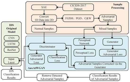
Figure 1.
Block diagram of AuxAtWGAN.
The AuxAtWGAN architecture combines adversarial training, auxiliary networks, and generative adversarial networks (WGANs). An adversary-trained improved WGAN is employed to detect and remove adversarial samples from the dataset before they enter the original model, thereby enhancing the robustness of the intrusion detection system against adversarial attacks. The architecture aims to integrate the generator and discriminator to improve IDS detection in malicious attack scenarios by correcting and effectively classifying adversarial samples.
The AuxAtWGAN architecture is shown in Figure 2.
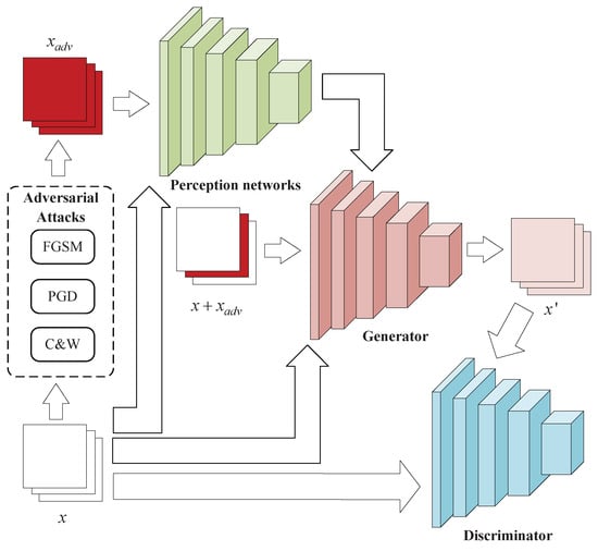
Figure 2.
Architecture of AuxAtWGAN.
The AuxAtWGAN architecture consists of the following key components:
- (1)
- Generator (G): The role of the generator is to receive the mixed samples that have been disturbed by the adversarial attack and map them close to normal samples. The generator aims to process the input data through a CNN to mitigate the adversarial perturbation and make the adversarial sample closer to the normal sample.
- (2)
- Discriminator (D): The discriminator of AuxAtWGAN is exclusively responsible for the categorization of adversarial samples, whereas the categorization of normal and attack samples is still carried out by the classifier of the original model. The discriminator’s function is to differentiate between normal and adversarial inputs. It extracts features from the input samples using a CNN architecture and performs classification.
- (3)
- Perceptual network (PN): The perceptual network calculates the perceptual loss between real samples. Through the perceptual loss, the generator helps optimize the adversarial samples, generates adversarial samples closer to the real samples, and ensures the consistency of the generated adversarial samples in the feature space.
To improve the original model’s robustness, data from its input layer are extracted and processed through the pretrained AuxAtWGAN to detect adversarial samples. Subsequently, detected adversarial samples are then removed, and the remaining data are re-input into the original model for intrusion detection.
3.2. AuxAtWGAN Model Design
3.2.1. SAE Data Downscaling
Since the mainstream models are image-based models, one-dimensional traffic data using an SAEis downscaled and converted to two-dimensional data in the data preprocessing stage.
Stacked autoencoders form a deeper model by connecting multiple autoencoder layers. The advantage over single-layer self-encoders is that layer-by-layer training captures deeper features of the input data, which effectively reduces the data dimensionality.
The training process involves the encoding of data from the input layer to the hidden layer and decoding from the hidden layer to the output layer. The encoding formula is as follows:
where h is the output of the encoder, x represents the original input data, represents the sigmoid activation function, and and represent the weights and biases of the encoder, respectively. The goal is to minimize the reconstruction loss as follows:
The decoding formula is as follows:
where is the output of the decoding layer, h is the input of the decoding layer, is the sigmoid activation function, and and are the weights and biases of the decoding layer.
The goal is to minimize the refactoring loss as follows:
The SAE model structure is shown in Figure 3.
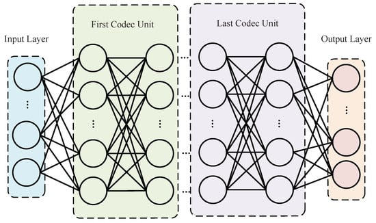
Figure 3.
SAE model structure.
After the SAE model extracts deeper features, the one-dimensional data are sliced and stacked into a two-dimensional format of , which is required by subsequent models.
3.2.2. Adversarial Sample Generation
Using only a specific adversarial training method produces an overfitting-like phenomenon during model training; this approach achieves high detection accuracy but suffers from poor generalization when other kinds of attack samples are not added to the adversarial training set. Therefore, three adversarial attacks, PGD [19], FGSM [31], and C&W [32] were used to generate adversarial samples and construct hybrid adversarial attack samples to achieve similar data augmentation and improve the generalizability of adversarial training.
1. The fast gradient sign method (FGSM)
The FGSM is an early gradient-based white-box adversarial attack method, swiftly generates adversarial samples to induce misclassification in deep learning models. It uses the gradient of the model’s loss function to generate perturbations that are applied to the input data to maximize the model’s classification error rate. The FGSM is a single-step gradient attack method that generates adversarial samples through a single gradient update. The core idea of the FGSM is to use the gradient of the neural network’s loss function to synthesize adversarial noise superimposed on pristine samples to manipulate the classification outcome of the victim network. With a single gradient computation, it achieves low computational cost and rapid generation.
Given a neural network classifier and real category labels y, its loss function is denoted as follows:
where is the original input sample, y is the true label, is the output of the neural network model, and is the loss function of the model.
The specific steps are as follows:
- (1)
- The gradient of the loss function is calculated with respect to the input x.
- (2)
- The adversarial samples are updated according to the direction of the gradient:where is the perturbation strength parameter that controls the maximum differences between the antagonistic sample and the original sample.
2. Projected gradient descent (PGD)
PGD is a method based on gradient iteration. PGD is based on an -constrained adversarial attack, and its core idea is to generate adversarial samples step by step through multiple small step gradient updates while restricting the perturbation to a certain range.
PGD optimizes the following objectives:
where is the sphere centered at x with radius . The sphere is used as a boundary to constrain the size of the perturbation.
By performing random initialization before the adversarial samples are generated, a random point is selected as the initial perturbation sample and ensured to be in the neighborhood of , so it can jump out of the local optimal solution by random initialization to improve the attack effect. The random initialization formula is as follows:
Moreover, the PGD attack ensures that the adversarial samples do not exceed the perturbation range by constraining the projection, with the cropping formula as follows:
The perturbations beyond are cropped to and via the above equation, which limits the perturbation size.
The specific steps are as follows:
- (1)
- The adversarial sample is randomly initialized to the original sample x, or its vicinity is randomly perturbed.
- (2)
- In each iteration, the gradient of the loss function concerning the input x is computed as .
- (3)
- The adversarial samples are updated according to the direction of the gradient:where is the step size, is the upper limit of the perturbation, and ensures that the generated adversarial samples are within the allowed perturbation range.
- (4)
- This optimization loop terminates when either the predefined iteration limit is exhausted, or the desired adversarial condition is achieved.
3. Carlini and Wagner (C&W)
The C&W attack differs from gradient symbol-based methods such as the FGSM or PGD as it identifies minimal distortions via iterative refinement to induce input misclassification while preserving perceptual consistency between adversarial examples and pristine data. As an optimization-driven attack, the C&W framework prioritizes the objective function’s calibration, enabling crafted inputs to both evade detection and retain fidelity to the original sample.
A C&W attack is essentially a constrained optimization problem:
where is the added perturbation, is the norm of the perturbation, is the output of the target classifier, is the attacking target class, and is constrained to ensure that the antagonistic sample values remain within the valid input range.
To make the objective optimization problem differentiable, C&W uses a Lagrangian relaxation method to introduce an auxiliary objective function:
where c is the trade-off parameter used to adjust the trade-off between the size of the perturbation and the success rate of the attack, and is the loss of the classification of the attack target, with the following formula:
where is the logit value of the target category, is the maximum logit value other than the target category, is the confidence level, and increasing can increase the success rate of the attack at the cost of increasing the perturbation.
The detailed procedure is as follows:
- (1)
- First, for the stability of the optimization, the variable substitution method is used:where w is an optimized variable that replaces to ensure that x is in the range .
- (2)
- The appropriate perturbation is then found by optimizing the variable w with Equation (12).
- (3)
- Finally, w is optimized iteratively using the Adam optimizer until the smallest perturbation that can trick the model is found or the maximum number of iterations is reached.
3.2.3. WGAN
In traditional GANs, the JS divergence is used to measure the difference between the generated and real data distributions ( and ). The optimization of GANs is often unstable and susceptible to mode collapse due to the vanishing gradient problem associated with the JS divergence, leading the generator to produce a limited variety of samples and not fully represent the data distribution. The WGAN employs the Wasserstein distance as its optimization objective, enhancing training stability and the quality of generated data. The Wasserstein distance is used to measure the optimal transport cost between two probability distributions, i.e., the lowest cost required to transform from one distribution to another, and is defined as follows:
where represents the real data distribution, represents the generated data distribution, and represents the set of all joint distributions such that their marginal distributions are and .
The Wasserstein distance offers superior mathematical properties over the JS divergence, leading to a more stable discriminator gradient and effectively guiding generator optimization to prevent the vanishing gradient issue during training.
The goal of the WGAN is to minimize the Wasserstein distance, with its optimization objective specified as:
where represents the discriminator’s output, which is no longer a probability value as in the traditional GAN but rather a real score that measures the sample’s truth. The discriminator D needs to maximize the Wasserstein distance between the real data x and the generated data , and the generator G makes the generated samples as similar as possible to the real samples by minimizing the score of the discriminator.
By minimizing the discriminator’s score, the generator makes the generated samples as similar as possible to the real samples by maximizing the Wasserstein distance between the real data x and the generated data .
In order to enhance the stability of model training and circumvent the vanishing gradient problem, a gradient penalty is employed to supersede the weight clipping strategy in the original WGAN [33]. The computation of the Wasserstein distance requires that the discriminator satisfies Lipschitz continuity:
To satisfy this condition, the WGAN employs the gradient penalty method’s gradient penalty term for the optimization:
where serves as a balancing factor to adjust the gradient penalty magnitude, and where denotes a probabilistic mixture of the original sample x and the generated sample .
Therefore, the objective function is rewritten as shown in the following equation:
The adversarial training process of the auxiliary model differs from that of the original model, and its training goal is to optimize its classification ability using the guidance of the adversarial samples according to the features extracted from the original model. During training, the auxiliary model continuously adjusts its parameters to recognize small changes caused by perturbations on the basis of known attack samples and normal samples. In this process, the sensitivity of the auxiliary model to perturbations is improved by continuously optimizing the representation of the feature space, thereby enhancing the robustness of the entire system itself.
3.2.4. Generator
The main task of the generator in the AuxAtWGAN architecture is to receive adversarial samples and correct them. The key features of the attack traffic are preserved while remaining as close as possible to the normal traffic data.
The generator architecture is shown in Figure 4.

Figure 4.
Architecture of the generator.
The core architecture of the generator uses a CNN with a structure consisting of a stack of three convolutional layers and three anticonvolutional layers. Convolutional layers extract features from input data, while inverse convolutional layers reconstruct the data to restore generated traffic samples to a clean distribution. In terms of network design, features are first extracted from the input data by multiple convolutional layers to obtain a low-dimensional but highly expressive feature representation that is subsequently upsampled by the inverse convolutional layers to gradually recover the spatial dimension of the input data. To improve training stability and sample quality, the generator’s middle layer utilizes batch normalization and a leaky ReLU activation function. This approach addresses the vanishing gradient issue, accelerates model convergence, and enhances sample diversity.
During the training process of the generator, AuxAtWGAN uses a combination of adversarial loss and perceptual loss to ensure that the generated traffic samples can both deceive the discriminator and maintain similarity to the real data at the high-level feature level. Adversarial loss evaluates if generated samples can effectively deceive the discriminator by resembling normal data, while perceptual loss assesses the feature space discrepancy between generated samples and actual normal traffic data. This ensures that generated samples are not only pixel-wise similar but also align closely with real samples in high-level feature representations. The computation of the perceptual loss relies on a pretrained convolutional neural network to optimize the quality of the generator’s output by comparing the Euclidean distances between the generated samples and the normal samples at the feature level.
The generator loss formula is as follows:
where is the generator loss of the WGAN, represents the adversarial sample generated by the generator, represents the sample distribution of the generator, represents the discriminator’s output value for the generated sample , which is used to represent the similarity between the generated sample and the real data, and represents the perceptual loss, which measures the difference between the generated sample and the real sample x in the deep layer of the feature space.
Using the tanh activation function, the final output layer normalizes the traffic data to the range to match the original distribution. The training objective of the entire generator is to minimize the perceptual loss of its generated samples concerning the normal traffic samples and simultaneously maximize its adversarial loss so that the generated samples can deceive the discriminator.
3.2.5. Perception Networks
Conventional loss functions usually capture only low-level pixel-level differences and do not reflect the visual quality of an image in high-level features, especially the small perturbations generated by the adversarial sample generation algorithm. To overcome this problem, AuxAtWGAN introduces perceptual networks that guide the generator to produce adversarial samples that are more natural and closer to real traffic by computing deeper feature differences. In the AuxAtWGAN model, the perceptual network enhances the generator’s output quality by aligning adversarial samples with normal traffic data both at the pixel level and within the deeper high-level feature space.
The perceptual network employs a pretrained convolutional neural network to derive high-level features from input samples. The generator of the GAN relies only on traditional pixel-level comparisons, whereas the perceptual network computes the difference by comparing the feature representations of the generated samples with those of the real samples in the convolutional neural network. This method more accurately captures the perceptual differences between generated and real samples, particularly regarding texture, edge, and shape similarity. Minimizing perceptual loss enhances the generator’s ability to produce samples that closely resemble real samples in terms of high-level features. The architecture primarily consists of convolutional, pooling, and fully connected layers. Specifically, the architecture comprises convolutional layers and max pooling layers, which are arranged in a three-layer configuration. Subsequently, a flattening layer, dropout layer, and fully connected layer with sigmoid activation are applied. There are 10 hidden layers in the network, not counting the input and output layers.
The perceptual networks architecture is shown in Figure 5.
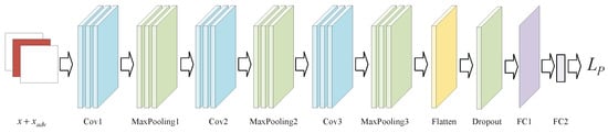
Figure 5.
Architecture of the perceptual networks.
The formula for calculating the perceived loss is as follows:
where the distributions denote the feature representations of the generated and real samples extracted by the pretrained neural network at layer j, and the square of the Euclidean distance between them represents the difference between the two samples. and denote the height and width of the features in layer j.
The introduction of perceptual networks allows the generator to be optimized not only at low-level pixel differences but also, more importantly, at high-level feature levels to maintain the similarity between generated and normal samples. The features of the adversarial samples in the data are usually difficult to observe at the low-level pixels, and the normalcy and aggressiveness of the traffic can be represented only by high-level feature extraction.
In addition, the perceptual network also helps to denoise and enhance data quality. Minimizing perceptual loss enables the generator to produce adversarial samples that are visually and structurally similar to normal traffic in the high-level feature space. This process aids the generator in handling complex samples and creating more natural adversarial samples.
3.2.6. Discriminator
In the AuxAtWGAN model, the discriminator’s primary role is to identify if input samples are adversarial ones corrected by the generator, rather than classifying them as ‘normal traffic’ or ‘attack traffic’. Therefore, the discriminator needs to recognize only whether the input data are attack-generated adversarial samples instead of directly classifying the network traffic. This design streamlines the model’s complexity, enabling the discriminator to concentrate more effectively on classifying adversarial samples.
The discriminator architecture is shown in Figure 6.
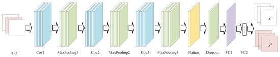
Figure 6.
Architecture of the discriminator.
The discriminator employs a CNN network with the same architecture as the perceptual network. The discriminator utilizes these layers to extract relevant features from data streams, enabling it to identify if a sample is adversarially generated. The convolution part detects shapes and textures by scanning local areas, the pooling part makes the data smaller to speed up calculations, and the connected layers put everything together to choose the output label.
The input to the discriminator consists of two types of samples: normal traffic samples from the original traffic dataset and the output obtained by the generator by correcting the adversarial samples. The goal of the discriminator is to output a probability value indicating whether the input sample is adversarial; if it is an adversarial sample, the output is close to 0; otherwise, the output is close to 1.
In training, the discriminator’s loss function primarily includes adversarial loss, aimed at minimizing its error in distinguishing between adversarial and normal samples. The discriminator enhances its capability to identify adversarial samples by minimizing the loss between these generated samples and real ones. Optimizing the loss function enhances the discriminator’s ability to accurately identify adversarial samples, ensuring the generator effectively ‘deceives’ the discriminator with its outputs. The specific formula is as follows:
where is the classification loss, which indicates the classification loss for real and generated samples. is the discriminative loss, which represents the discriminator’s ability to distinguish between real samples and generated samples.
The categorized loss formula is as follows:
where represents the discriminator’s prediction score, and where corresponds to the cross-entropy loss function, quantifying the discrepancy between the model’s predictions and the truth labels.
The discriminator loss formula is as follows:
where is the output of the discriminator for the real samples, and where is the output of the discriminator for the generated samples.
The design and optimization of the discriminator is a core component of the AuxAtWGAN model, which functions with the generator. The generator’s goal is to generate as many realistic adversarial samples as possible to deceive the discriminator, while the discriminator improves the model’s sensitivity to adversarial features by continuously improving the recognition accuracy. Through this alternating optimization training process, the discriminator can eventually effectively detect the adversarial samples corrected by the generator and enhance the robustness to adversarial attacks.
4. Experiments
4.1. Dataset
The CICIDS-2017 dataset provides a testbed that is similar to real-world network environments for research on intrusion detection systems [34]. The large-scale nature of the CICIDS-2017 data allows researchers to train complex machine learning models and perform in-depth statistical analysis. The dataset’s 78 multidimensional features, spanning 15 attack categories, offer extensive options for developing precise and robust detection models. The category imbalance problem between attack data and normal traffic data in the dataset reflects the scarcity of attack traffic in the real world.
4.2. Evaluation Indicators
Four cases of model classification results were considered:
- True Positive (TP): the count of samples accurately identified as belonging to the positive category.
- False Positive (FP): the count of negative samples mistakenly classified as positive.
- True Negative (TN): the count of instances accurately identified as belonging to the negative category when they indeed belong there.
- False Negative (FN): the count of positive samples mistakenly classified as negative.
To evaluate the model’s robustness, the accuracy (ACC) and attack success rate (ASR) were used. The ACC was used to evaluate the classification ability of the model before and after a model attack and can be expressed as shown in Equation (26):
The ASR is a commonly used metric for evaluating attack effectiveness in the study of adversarial attacks [35].
where denotes the total number of samples in the test dataset, and denotes the number of samples that were successfully attacked. A higher ASR means that the attack is more effective against the model and that the model is less robust.
4.3. Experimental Configuration
The experiment used the Windows 11 system, the Python 3.9 programming language, the PyCharm development environment, and the PyTorch 1.12.1 deep learning framework. An AMD Ryzen7 6800H processor, an RTX 3070Ti (8 G) graphics card, and 16 GB of DDR4 memory were used.
The deep learning models used for the experiments were as follows:
- Convolutional neural network (CNN): a CNN is good at processing data with spatial local correlation of two-dimensional grayscale images. The feature extraction of two-dimensional network traffic data after SAE conversion was used for comparison with the WGAN model used. The CNN model structure was the same as the discriminator structure.
- Long Short-Term Memory (LSTM): LSTM is a very suitable neural network model for partitioning one-dimensional time series data, such as network traffic data. Consequently, LSTM was chosen for its prevalent application in time series analysis within intrusion detection systems. The LSTM network used for the experiment consisted of two layers consisting of an LSTM layer, a dropout layer, and fully connected layers. The model could better capture the time-dependent features in the sequence data and improve the performance of the classification task.
- Residual Neural Network (ResNet): As a representative of deep networks, the method could be tested for its adaptability to deeper and more complex models and compared with LSTM in terms of spatial and temporal features. ResNet34 contains an initial convolutional layer; four residual layers with three, four, six, and three residual modules in each layer; and a fully connected layer [36].
The models were trained with the Adam optimizer, using cross-entropy loss, a batch size of 128, a learning rate of 0.001, over 50 epochs, and a dropout rate of 0.3.
The adversarial attack parameters were as follows:
- FGSM: ;
- PGD: , , ;
- C&W: , .
4.4. Experiment Results and Discussion
4.4.1. SAE and Data Visualization Results
The CICIDS2017 dataset has 78 features; after SAE data dimensionality reduction to 64 features of one-dimensional data, the data were sliced and stacked into an format. The first four classification samples after data visualization are shown in Figure 7.
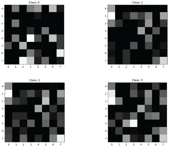
Figure 7.
Visualization of SAE sample data.
After conversion to grayscale images a normalization process was performed to linearly map the pixel intensities to the normalized interval . Within this range, the values are strictly positively correlated with the luminance, 0.0 means pure black, 1.0 means pure white, and intermediate values correspond to different depths of grey.
4.4.2. Generating Adversarial Sample Results
To visualize the FGSM, PGD and C&W generate adversarial samples for confrontation, the corresponding samples are selected to be converted to grayscale maps for visualization and to show the original samples, the adversarial samples, and the perturbations, respectively, and similarly 0.0 denotes pure black, 1.0 denotes pure white, and the intermediate values correspond to different depths of gray.
The FGSM generated adversarial samples as shown in Figure 8.
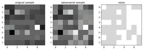
Figure 8.
Adversarial samples generated via the FGSM.
The original sample is on the left, the generated adversarial sample is in the center, and the noise with added perturbations is on the right.
PGD generated adversarial samples as shown in Figure 9.
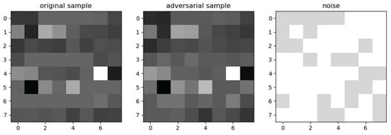
Figure 9.
Adversarial samples generated via PGD.
C&W generated adversarial samples as shown in Figure 10.
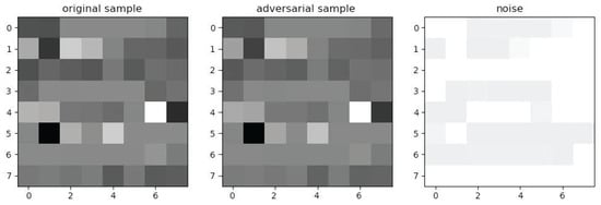
Figure 10.
Adversarial samples generated via C&W.
4.4.3. AuxAtWGAN Comparison Experiments
The AuxAtWGAN scheme was examined to balance normal sample classification accuracy with adversarial sample detection capability. The proportions of 10%, 20%, and 50% adversarial samples were selected to simulate adversarial perturbation environments with different strengths, and the model’s adaptive ability at each proportion was evaluated. The experimental findings identified the ideal ratio of adversarial samples needed to effectively detect them while maintaining high classification accuracy for normal samples.
To generate samples with different proportions, we initially selected a random subset of the original samples. Subsequently, we generated adversarial samples for these original samples using FGSM, PGD, and C&W methods sequentially, ensuring an equal number of adversarial samples from each method. To ensure the correct proportion of mixed samples, 11%, 25% and all (100%) of the normal samples were selected to generate adversarial samples, respectively.
The results in Table 1 show that when the adversarial sample proportions were 10%, 20%, and 50% with AuxAtWGAN, the original model still maintained high accuracy due to little change in the accuracy of the original model for normal samples with the auxiliary model approach used, but the model with the discriminator input and 50% adversarial samples had the highest detection accuracy of 85.73% for adversarial samples. Because a highly defensive auxiliary model must be obtained, the proportion of adversarial samples in the subsequent experiments was set to 50%.

Table 1.
Accuracies of classifying normal and adversarial samples with different proportions.
The study evaluated the impact of baseline, adversarial training (AT), and AuxAtWGAN methods on the classification accuracy of both normal and adversarial samples. The baseline model was a standard WGAN network. AT refers to a WGAN network trained adversarially alongside the baseline. The proposed method in this paper is AuxAtWGAN, while CNN+AT denotes a CNN model trained adversarially. The experiment aimed to assess the effect of adversarial training on improving model robustness and examine its potential influence on standard classification performance. Furthermore, the auxiliary model’s role was examined to assess its ability to preserve the original model’s classification performance on normal samples while improving robustness.
The classification accuracy curves for normal and adversarial samples via the different methods are shown in Figure 11 and Figure 12.
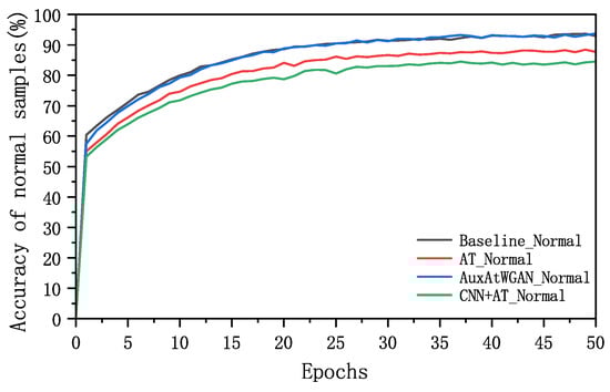
Figure 11.
Accuracy of the original model for classifying normal samples with different methods.
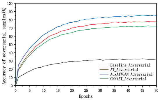
Figure 12.
Classification accuracy for adversarial samples via different methods.
In Figure 12, the experimental results show that the detection rate of the completely unguarded baseline method for adversarial samples was very low, while the AT and CNN+AT methods after adversarial training significantly improved the defense ability of the adversarial samples, and compared with the method with adversarial training, the AuxAtWGAN method with the WGAN and perceptual network augmentation achieved a certain improvement in terms of the defense effect. A comparison of the accuracies of the baseline, AT, CNN+AT, and AuxAtWGAN methods for normal and adversarial samples is shown in Table 2.
Table 2.
Comparison of the accuracies for normal and adversarial samples.
The results in Table 2 show that adversarial training significantly improved the model’s classification performance for adversarial samples, and the accuracy for the adversarial samples was increased to 78.16% compared with the 32.49% accuracy of the baseline, whereas the accuracy of adversarial samples of AT and CNN+AT decreased slightly compared with that of normal samples, indicating that adversarial training negatively affected the detection performance for the normal samples while improving the robustness. Integrating the auxiliary model enhanced robustness, achieving a classification accuracy of 93.57% for normal samples and 85.77% for adversarial samples.
To further validate the reliability of the AuxAtWGAN method at the level of statistical significance, we determined 95% confidence intervals (CIs). The previous experiments showed that AuxAtWGAN exhibited significant advantages in both adversarial sample detection and normal sample classification, but the confidence intervals need to be derived for the experimental results to exclude the influence of random fluctuations. The stability and repeatability of the model performance can be quantitatively assessed by calculating the mean and standard deviation of the normal sample classification accuracy and the adversarial sample detection accuracy and constructing 95% confidence intervals based on the t-distribution. The random seeds were selected as 0, 42, 2025, 8888, 9527, and the results are shown in the Table 3:
Table 3.
95% Confidence interval analysis of AuxAtWGAN performance.
The AuxAtWGAN achieved 93.57% accuracy on normal samples and 85.73% accuracy on adversarial samples, with tight 95% confidence intervals, [93.37%, 93.77%] and [85.35%, 86.12%]. The low standard deviations (0.23% for normal, 0.44% for adversarial) confirmed the stable performance across repeated experiments. The non-overlapping confidence intervals highlighted statistically significant differences between normal and adversarial results, validating the model’s ability to maintain high accuracy on normal traffic while under adversarial attacks.
The attack success rates of the baseline, AT, and AuxAtWGAN methods were compared against attack methods alone via the PGD, FGSM, and C&W methods, respectively. The goal of this experiment was to verify the adaptability of different defense strategies to different attack methods, especially to evaluate whether the auxiliary model could further reduce the attack success rate, thus enhancing the overall robustness of the IDS in multiple attack environments. The experimental results are shown in Table 4.
Table 4.
Comparison of defense effects against multiple attacks.
Table 4 demonstrates that adversarial training markedly lowered the model’s vulnerability to various adversarial attacks, reducing the average attack success rate from 75.17% to 33.40% compared to the baseline. When combined with the auxiliary model, the average attack success rate further decreased to 27.56%. The auxiliary model enhanced the model’s robustness against adversarial attacks by learning adversarial sample features through adversarial training.
The generalizability of the AuxAtWGAN method was assessed by evaluating its defense effectiveness against that of LSTM and ResNet34 models using five types of input samples: normal samples, mixed samples, FGSM, PGD, and C&W adversarial samples. The experiments were conducted using four models, namely, LSTM, ResNet34, LSTM+AuxAtWGAN and ResNet34+AuxAtWGAN. The normal sample set evaluated the original model’s classification performance on non-attacked samples, while the hybrid sample set, comprising FGSM, PGD, and C&W adversarial samples, assessed the model’s robustness. The FGSM, PGD, and C&W adversarial samples, each representing distinct attack modes, were utilized to evaluate the model’s defense capabilities. The experiment used accuracy to assess model performance across different sample types. Figure 13 presents the experimental results.
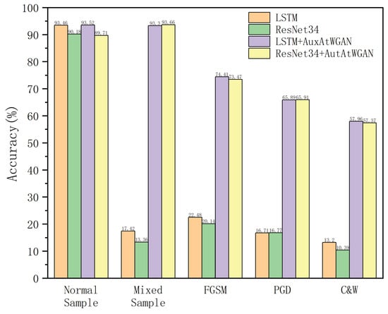
Figure 13.
Classification accuracy of LSTM and ResNet34 with and without the auxiliary AuxAtWGAN.
In Figure 13, the experimental results show that the classification accuracy for normal samples was almost unaffected. The accuracies of LSTM+AuxAtWGAN and LSTM on normal samples were 93.52% and 93.46%, respectively, and those of ResNet34+AuxAtWGAN and ResNet34 reached 89.71% and 90.18%, respectively. This showed that AuxAtWGAN, as an auxiliary module, did not affect the original model’s ability to classify normal samples, and its introduction did not degrade the original performance of the model.
In the mixed-sample test, the accuracies of LSTM and ResNet34 drastically decreased to only 17.42% and 13.36%, respectively, because of the lack of adversarial training. In contrast, LSTM+AuxAtWGAN achieved an accuracy of 93.30% on the mixed samples, indicating that AuxAtWGAN enabled the model to maintain a high classification accuracy in mixed data environments by learning the feature distribution of the adversarial samples. The experiments on ResNet34 in Section 3 demonstrated weaker robustness than those on LSTM, with an accuracy of 13.36%, whereas ResNet34+AuxAtWGAN achieved an accuracy of 93.66%, indicating that AuxAtWGAN could further optimize the classification performance for adversarial samples on the basis of the stronger base model.
In the adversarial sample test, LSTM was more capable of defending against adversarial attacks, with accuracy rates of 22.48%, 16.71%, and 13.20% from the FGSM, PGD, and C&W attacks, respectively. In contrast, the accuracy of LSTM+AuxAtWGAN reached 74.41%, 65.89%, and 57.96%, indicating that AuxAtWGAN could effectively identify and resist adversarial samples and improve the model’s adversarial robustness. For ResNet34, the accuracies were 20.14%, 16.77%, and 10.39% from the three attacks. After AuxAtWGAN was attacked, the accuracy improved to 73.4%, 65.9%, and 57.3%, which indicated that AuxAtWGAN could further optimize the defense performance of the existing model and achieve better generalizability.
5. Conclusions
This work proposed an intrusion detection system that enhanced robustness on the basis of adversarial training to generate a new adversarial network, AuxAtWGAN. The network combined the advantages of two defense strategies, namely, auxiliary modeling and adversarial training, to increase the effectiveness and generalizability performance of the deep learning model in the face of adversarial attacks.
- (1)
- Firstly, the SAE network traffic data were downscaled by the SAE and transformed into 2D data suitable for model processing, and mixed adversarial samples were generated by the FGSM, PGD, and C&W adversarial attack methods, which significantly increased the diversity of adversarial training data and improved the generalization ability of the model. Data were then visualized to directly observe the perturbation effects on the samples.
- (2)
- Secondly, the normal samples and the mixed adversarial samples were used as hybrid samples, which were fed into the AuxAtWGAN proposed in this paper. The feature space consistency of the generator was maintained through perceptual loss constraints, and adversarial training utilizing the generative network optimized the correction quality of the adversarial samples, thus improving the adversarial sample detection accuracy to 85.77%.
- (3)
- Finally, the pretrained model can be attached to various deep learning models to eliminate the adversarial samples in the input data and improve robustness. Maintaining the original model’s detection accuracy for normal samples resulted in a reduction in the average attack success rate from 75.17% to 27.56%. The strong generalizability of the model was validated on models such as LSTM and ResNet.
Although some progress was made in IDS robustness assessment and defense, several shortcomings remain:
- (1)
- Firstly, the current defense methods are based mainly on adversarial training and auxiliary networks, which improve robustness but still rely on known adversarial samples. In the future, the introduction of an adaptive defense mechanism can be considered so that the IDS can dynamically adjust the adversarial training strategy and improve the defense ability against unknown attacks.
- (2)
- Secondly, adversarial defense methods have some overhead in computational resources, especially the WGAN training process, which is more complicated. In the future, knowledge distillation or pruning techniques can be explored to optimize the model in a lightweight way so that it can operate efficiently in resource-constrained environments.
- (3)
- Finally, the current experiments are based on public datasets such as CICIDS-2017 and still need to be further verified for applicability in real network environments. In the future, IDSs can be deployed in real application scenarios, and their robustness and detection performance in dynamic traffic environments can be evaluated.
Author Contributions
Conceptualization, G.W. and Q.Y.; methodology, G.W. and Q.Y.; software, G.W. and Q.Y.; validation, G.W. and Q.Y.; formal analysis, G.W. and Q.Y.; investigation, G.W. and Q.Y.; data curation, G.W. and Q.Y.; writing—original draft preparation, Q.Y. and G.W.; writing—review and editing, Q.Y. and G.W.; visualization, Q.Y.; supervision, G.W. All authors have read and agreed to the published version of the manuscript.
Funding
This work was supported by the Gansu Provincial Science and Technology Program Grant 25JRRA190, in part by the Gansu Provincial Department of Education Industry Support Project 2022CYZC-38.
Institutional Review Board Statement
Not applicable.
Informed Consent Statement
Not applicable.
Data Availability Statement
The CICIDS2017 dataset utilized in this research is accessible to the public. It is located at the following URL: https://www.unb.ca/cic/datasets/ids-2017.html (accessed on 28 February 2025).
Acknowledgments
The authors would like to thank Lanzhou Jiaotong University for supporting this work. They would also like to thank the reviewers for their invaluable input that helped improve the paper.
Conflicts of Interest
The authors declare no conflicts of interest.
References
- Anderson, J.P. Computer Security Threat Monitoring and Surveillance; Technical report; James P. Anderson Company: Fort Washington, PA, USA, 1980. [Google Scholar]
- Lansky, J.; Ali, S.; Mohammadi, M. Deep learning-based intrusion detection systems: A systematic review. IEEE Access 2021, 9, 101574–101599. [Google Scholar] [CrossRef]
- Farahnakian, F.; Heikkonen, J. A deep auto-encoder based approach for intrusion detection system. In Proceedings of the 20th International Conference on Advanced Communication Technology (ICACT), Chuncheon-si, Republic of Korea, 1–14 February 2018; pp. 178–183. [Google Scholar]
- Szegedy, C.; Liu, W.; Jia, Y. Going deeper with convolutions. In Proceedings of the IEEE Conference on Computer Vision and Pattern Recognition (CVPR), Boston, MA, USA, 7–12 June 2015; pp. 1–9. [Google Scholar]
- Mohammadpour, L.; Ling, T.C.; Liew, C.S.; Aryanfar, A. A survey of CNN-based network intrusion detection. Appl. Sci. 2022, 12, 8162. [Google Scholar] [CrossRef]
- Hochreiter, S.; Schmidhuber, J. Long short-term memory. Neural Comput. 1997, 9, 1735–1780. [Google Scholar] [CrossRef] [PubMed]
- Laghrissi, F.; Douzi, S.; Douzi, K.; Hssina, B. Intrusion detection systems using long short-term memory (LSTM). J. Big Data 2021, 8, 65. [Google Scholar] [CrossRef]
- Guo, J.; Bao, W.; Wang, J.; Ma, Y.; Gao, X.; Xiao, G.; Wu, W. A comprehensive evaluation framework for deep model robustness. Pattern Recognit. 2023, 137, 109308. [Google Scholar] [CrossRef]
- Sauka, K.; Shin, G.Y.; Kim, D.W.; Han, M.M. Adversarial robust and explainable network intrusion detection systems based on deep learning. Appl. Sci. 2022, 12, 6451. [Google Scholar] [CrossRef]
- Zhang, S.; Chen, S.; Liu, X.; Hua, C.; Wang, W.; Chen, K.; Wang, J. Detecting adversarial samples for deep learning models: A comparative study. IEEE Trans. Netw. Sci. Eng. 2021, 9, 231–244. [Google Scholar] [CrossRef]
- Yang, K.; Liu, J.; Zhang, C.; Fang, Y. Adversarial examples against the deep learning based network intrusion detection systems. In Proceedings of the MILCOM 2018—2018 IEEE Military Communications Conference (MILCOM), Los Angeles, CA, USA, 29 October–1 November 2018; pp. 559–564. [Google Scholar]
- Arjovsky, M.; Chintala, S.; Bottou, L. Wasserstein generative adversarial networks. In Proceedings of the 34th International Conference on Machine Learning (ICML), Sydney, Australia, 6–11 August 2017; PMLR: Sydney, Australia, 2017; Volume 70, pp. 214–223. [Google Scholar]
- Yan, B.; Han, G. Effective feature extraction via stacked sparse autoencoder to improve intrusion detection system. IEEE Access 2018, 6, 41238–41248. [Google Scholar] [CrossRef]
- Pan, Y.; Pi, D.; Chen, J.; Meng, H. FDPPGAN: Remote sensing image fusion based on deep perceptual patchGAN. Neural Comput. Appl. 2021, 33, 9589–9605. [Google Scholar] [CrossRef]
- Zhao, W.; Alwidian, S.; Mahmoud, Q.H. Adversarial training methods for deep learning: A systematic review. Algorithms 2022, 15, 283. [Google Scholar] [CrossRef]
- He, K.; Kim, D.D.; Asghar, M.R. Adversarial machine learning for network intrusion detection systems: A comprehensive survey. IEEE Commun. Surv. Tutor. 2023, 25, 538–566. [Google Scholar] [CrossRef]
- Li, Y.; Cheng, M.; Hsieh, C.J.; Lee, T.C. A review of adversarial attack and defense for classification methods. Am. Stat. 2022, 76, 329–345. [Google Scholar] [CrossRef]
- Goodfellow, I.J.; Shlens, J.; Szegedy, C. Explaining and harnessing adversarial examples. In Proceedings of the 3rd International Conference on Learning Representations (ICLR), San Diego, CA, USA, 7–9 May 2015. [Google Scholar]
- Madry, A.; Makelov, A.; Schmidt, L.; Tsipras, D.; Vladu, A. Towards deep learning models resistant to adversarial attacks. In Proceedings of the 6th International Conference on Learning Representations (ICLR), Vancouver, BC, Canada, 30 April–3 May 2018. [Google Scholar]
- Bai, T.; Luo, J.; Zhao, J.; Wen, B.; Wang, Q. Recent advances in adversarial training for adversarial robustness. In Proceedings of the 30th International Joint Conference on Artificial Intelligence (IJCAI-21), Montreal, QC, Canada, 19–27 August 2021; pp. 4312–4321. [Google Scholar]
- Chauhan, R.; Sabeel, U.; Izaddoost, A.; Shah Heydari, S. Polymorphic adversarial cyberattacks using WGAN. J. Cybersecur. Priv. 2021, 1, 767–792. [Google Scholar] [CrossRef]
- Shieh, C.S.; Nguyen, T.T.; Lin, W.W.; Huang, Y.L.; Horng, M.F.; Lee, T.F.; Miu, D. Synthesis of adversarial DDoS attacks using Wasserstein generative adversarial networks with gradient penalty. In Proceedings of the 2021 6th International Conference on Computational Intelligence and Applications (ICCIA), Xiamen, China, 11–13 June 2021; IEEE: Piscataway, NJ, USA, 2021; pp. 118–122. [Google Scholar]
- Yu, Y.; Yu, P.; Li, W. Auxblocks: Defense adversarial examples via auxiliary blocks. In Proceedings of the 2019 International Joint Conference on Neural Networks (IJCNN), Budapest, Hungary, 14–19 July 2019; IEEE: Piscataway, NJ, USA, 2019; pp. 1–8. [Google Scholar]
- Samangouei, P.; Kabkab, M.; Chellappa, R. Defense-GAN: Protecting classifiers against adversarial attacks using generative models. In Proceedings of the 6th International Conference on Learning Representations (ICLR), Vancouver, BC, Canada, 30 April–3 May 2018. [Google Scholar]
- Jin, G.; Shen, S.; Zhang, D.; Dai, F.; Zhang, Y. APE-GAN: Adversarial perturbation elimination with GAN. In Proceedings of the 2019 IEEE International Conference on Acoustics, Speech and Signal Processing (ICASSP), Brighton, UK, 12–17 May 2019; pp. 3842–3846. [Google Scholar]
- Wang, D.; Jin, W.; Wu, Y.; Khan, A. ATGAN: Adversarial training-based GAN for improving adversarial robustness generalization on image classification. Appl. Intell. 2023, 53, 24492–24508. [Google Scholar] [CrossRef]
- Song, R.; Huang, Y.; Xu, K.; Ye, X.; Li, C.; Chen, X. Electromagnetic inverse scattering with perceptual generative adversarial networks. IEEE Trans. Comput. Imaging 2021, 7, 689–699. [Google Scholar] [CrossRef]
- Mahmoud, M.; Kang, H.S. Ganmasker: A two-stage generative adversarial network for high-quality face mask removal. Sensors 2023, 23, 7094. [Google Scholar] [CrossRef] [PubMed]
- Papernot, N.; McDaniel, P.; Wu, X.; Jha, S.; Swami, A. Distillation as a defense to adversarial perturbations against deep neural networks. IEEE Trans. Neural Netw. Learn. Syst. 2016, 27, 1631–1643. [Google Scholar]
- Lyu, C.; Huang, K.; Liang, H.N. A unified gradient regularization family for adversarial examples. In Proceedings of the 2015 IEEE International Conference on Data Mining (ICDM), Atlantic City, NJ, USA, 14–17 November 2015; pp. 301–309. [Google Scholar]
- Kurakin, A.; Goodfellow, I.J.; Bengio, S. Adversarial machine learning at scale. In Proceedings of the International Conference on Learning Representation (ICLR), Toulon, France, 24–26 April 2017. [Google Scholar]
- Carlini, N.W.; Wagner, D. Towards evaluating the robustness of neural networks. In Proceedings of the 2017 IEEE Symposium on Security and Privacy (SP), San Jose, CA, USA, 22–24 May 2017; pp. 39–57. [Google Scholar]
- Gulrajani, I.; Ahmed, F.; Arjovsky, M.; Dumoulin, V.; Courville, A.C. Improved training of Wasserstein GANs. Adv. Neural Inf. Process. Syst. 2017, 30, 5767–5777. [Google Scholar]
- Sharafaldin, I.; Lashkari, A.H.; Ghorbani, A.A. Toward generating a new intrusion detection dataset and intrusion traffic characterization. In Proceedings of the International Conference on Information Security and Privacy (ICISSP), Funchal, Portugal, 22–24 January 2018; pp. 108–116. [Google Scholar]
- Li, Y.; Jiang, Y.; Li, Z.; Xia, S.T. Backdoor learning: A survey. IEEE Trans. Neural Netw. Learn. Syst. 2022, 35, 5–22. [Google Scholar] [CrossRef] [PubMed]
- He, K.; Zhang, X.; Ren, S.; Sun, J. Deep residual learning for image recognition. In Proceedings of the IEEE Conference on Computer Vision and Pattern Recognition (CVPR), Las Vegas, NV, USA, 27–30 June 2016; pp. 770–778. [Google Scholar]
Disclaimer/Publisher’s Note: The statements, opinions and data contained in all publications are solely those of the individual author(s) and contributor(s) and not of MDPI and/or the editor(s). MDPI and/or the editor(s) disclaim responsibility for any injury to people or property resulting from any ideas, methods, instructions or products referred to in the content. |
© 2025 by the authors. Licensee MDPI, Basel, Switzerland. This article is an open access article distributed under the terms and conditions of the Creative Commons Attribution (CC BY) license (https://creativecommons.org/licenses/by/4.0/).