An Improved ADRC Parameters Self-Tuning Controller for Multi-Color Register System in Unit-Type Flexographic Printing Machines

Abstract

A self-tuning control strategy for Active Disturbance Rejection Control (ADRC) parameters based on a Radial Basis Function (RBF) neural network is proposed to improve the control accuracy of the roll-to-roll flexographic printing multi-color register system for its multi-input–multi-output and multi-span coupling characteristics. Firstly, according to the actual physical structure of flexographic printing equipment and the multi-physical coupling interface between adjacent spans, a mathematical model of the register system is established, and the multi-span coupling model is decoupled. Then, the ADRC decoupling controller is designed to estimate the disturbance and control the coupling model, and the RBF neural network is used to adjust the parameters of the decoupling controller in real time. Finally, the robustness, system decoupling, and anti-disturbance performance of the designed controller are verified under simulated steady speed and acceleration conditions. The simulation results show that the designed controller has better control performance than the conventional Proportional-Integral-Derivative (PID) and decoupled PID controllers. In steady state and accelerated simulations of PET/BOPP materials, respectively, the error peak is reduced by 86.7% and is controlled within ±10 μm, which satisfies the high-accuracy control requirements of the register system.

1. Introduction

The inline flexographic printing machines are widely used in the food and pharmaceutical fields, with the advantage of being green and environmentally friendly. However, its register system has the characteristics of strong coupling and strong interference, while its substrate materials include Polyethylene Terephthalate (PET), Biaxially Oriented Polypropylene (BOPP), Polyethylene (PE), Polyvinyl Chloride (PVC), etc., which makes it difficult to control the register accuracy under different printing environments and printing stages (the current control range of register error in the printing industry is ±20 μm). Therefore, there is an immediate requirement to solve the problem of decoupling and high-precision control of multi-color register systems in different printing scenarios.

The actual physical structure of the inline flexographic printing equipment is shown in Figure 1 (based on Solidworks 2019 software isometric drawing; key parameters are shown in

Table 1. Parameters of the model.

Machine Parameters	Value	Simulink Parameters	Value
Size	14 × 4 × 3	A	2.7 × 10−5 m2
Substrate	BOPP\PET	R1, R2, R3, R4	0.5 m
EBOPP (10 °C)	2.6 × 109 Pa	L1, L2, L3	5.05 m
EBOPP (20 °C)	2.24 × 109 Pa	T *	100 N
EBOPP (30 °C)	2.02 × 109 Pa	Ω *	1.66–3.32 m/s
EPET (20 °C)	4.89 × 109 Pa	E *	0 mm
		LD	1.8 m

* Note: Motor motion planning for PT mode, bottom roller, anilox roller, plate roller, and pressure regulation is directly driven by the motor.

), which consists of unwinding, infeeding, 4-color printing, oven system, outfeeding, rewinding, driving, and detection units (all 34 power units are directly driven by servo motors working in speed mode). In the actual printing process, longitudinal register errors are caused by changes in the speed of the printing plate roller, fluctuations in the material tension, delays in error detection, temperature variations in the drying system, and dynamic characteristics of the roller system. On the other hand, they are also influenced by factors such as manufacturing accuracy, assembly errors, and the performance of the motor drive. These errors are typical multi-source errors and are a major factor affecting printing register accuracy.

In addition to the synchronization system, the tension system and register system are important indicators for achieving high-fidelity printing. Stable control of tension is a prerequisite for registration. Most of the current research on tension modeling and control considers the effects of velocity, temperature, and mechanics based on the law of mass conservation and torque balance for multi-span modeling [1,2,3,4]. These methods are adopted to eliminate fluctuations in substrate tension, while the research on the register is mainly aimed at reducing register errors within the expected range from the angle of kinematics.

Register modeling and control are essential for achieving high-quality print. Existing studies consider factors such as speed, tension, and drying temperature to modulate the register, and then control it by improving Proportional-Integral-Derivative (PID) or modern control methods. Chen established the dynamic relationship between tension and register for the acceleration situation of the roll-to-roll printing system and proposed a feedforward Proportional-Derivative controller based on the Brandenburg 2-layer register model to converge the register error within ±0.1 mm [5,6,7]. Then, a model-based Fully Decoupled Proportional-Derivative control algorithm was proposed in [8] to achieve a fully decoupled system and control the register error within ±0.05 mm. Lee analyzed the effect of PET thermal and elastic deformation on the register error and established the error model by system identification techniques [9,10]. For this model, the inherent characteristics were considered in the design of the PI controller, and the register error was reduced to within ±0.03 mm at a printing speed of 0.033 m/s [11]. Then, to improve the controller response speed, a register controller based on Response Acceleration Input was proposed to control the register error within ±10 μm for PET material [12]. Kang developed a nonlinear model of a 3-layer register error with direct servo motor compensation based on the Brandenburg model, and applied feedforward control to offset the previous span error and control it within 75 μm for PET material at a speed of 0.5 m/s [13]. In addition to the adoption of controllers, the calibration of register errors from the perspective of mechanical structures is also being investigated. Kim used an active dance roll to eliminate the linear variation term of the register error [14]. Jung used an active motion-based roller combined with PID control for PET material to compensate for tension disturbances and material stretching and converge the register error to within 15 μm at a printing speed of 0.033 m/s [15]. Based on this, PID and feedforward control cannot meet the precision control requirements for register accuracy at high speeds. Our team’s research on register control established a nonlinear model and serially extended it to a multilayer register system, then proposed a control strategy of feedforward control combined with Active Disturbance Rejection Control (ADRC) technology to continuously control the register error within ±20 μm at a printing speed of 6.67 m/s [16]. The ADRC controller compensates for the disadvantages of PID controllers, such as unreasonable error extraction methods, insufficient dynamic margins, and inability to estimate unmodeled errors. However, in the actual printing environment, the working conditions are changing (frequently switching orders or performing acceleration and deceleration). Hence, the controller parameters need to be rectified to ensure the accuracy of register printing in real time. A Radial Basis Function (RBF) Neural Network is widely used for accurate real-time control of variable-parameter nonlinear systems with exogenous disturbances similar to register systems due to its strong generalization capability, fast convergence, and high approximation accuracy [17,18]. Meanwhile, the RBF neural network has better performance in servo motor control compared to other rectification methods (BP neural network) [19].

Aiming at the strong coupling problem of register systems in flexographic printing machines, this paper proposes a parameter self-tuning decoupling control strategy based on ADRC and RBF neural network. The structure of the article includes the following: In Section 2, the 4-color register system is modeled according to the actual physical structure of the flexographic printing machine to reveal the multi-coupling mechanism between adjacent spans, meanwhile decoupling the 4-color mathematical model. In Section 3, the parameters of the self-tuning decoupling controller is designed for the coupled model. Among them, ADRC is applied for perturbation estimation and dynamic compensation, and RBF neural network is used for real-time rectification of the ADRC controller parameters. In Section 4, the control performance of the designed decoupling controller is verified by comparison. In Section 5, a summary and directions for future work are given.

2. Mathematical Modeling of the Register System

The register system is mainly composed of the 4-color printing unit, oven system, and inspection components, which are coupled in series by substrate to form a multi-physical process coupled multi-input–multi-output system. Simplifying the whole machine structure, the 3-span register model structure is shown in Figure 2. To achieve high-fidelity printing, a multi-color register process based on the previous color is used (the first-color-based register process is not adopted), and the latter unit follows the previous unit to ensure a steady-state variation of the longitudinal register error at 0 by using a compatible monocular and binocular photoelectric eye (detection unit) for feedback of the error signal and consequently for speed adjustment of this unit.

In the actual printing process, the linear speed of the plate roller, anilox, and bottom roller is kept consistent, and the servo motor works in Permanent Torque (PT) mode. The virtual shaft is installed in the control system with the plate roller speed as the reference speed, and the anilox and bottom rollers do the following motion. To maintain a consistent linear speed, the number of motor pulses is given internally in the system to satisfy ω₁R₁ = ω_AR_A = ω_BR_B. Therefore, the following speeds ω_A and ω_B of the bottom roll and anilox roll are not considered in the model-building process.

2.1. Mathematical Model Establishment

Register error refers to the deviation in the position of different color marks that are intended to be printed in the same location. It is caused by changes in the substrate strain between two printed units, which results in a speed difference (a difference in the speed of the plate rollers) between the units and leads to displacement differences in the printed pattern further. The industry is commonly based on the material length Li between the two plate rollers as an integer multiple of the plate roller circumference to ensure accurate control of the register at a certain moment (pre-registration) and a specific coupling interface, as shown in Figure 3. According to the actual mechanical installation structure, the following are assumed: ① No strain occurs in the part of the material belt in contact with the plate roller, and the material properties of the substrate do not change. ② Between the substrate and the idler rollers, pure rolling and no sliding occur. ③ There is no other non-observable quantity for material transfer within the span of the substrate except for the inflow and outflow of ink; that is, the conservation of matter within the span is satisfied. ④ On the same substrate, at the same temperature, the strain of the substrate is equal everywhere.

Combined with Figure 3a, the process of register error is as follows: With the stamp point i − 1 at t₀ defined as the coordinate origin, in stage 1, the initial phase angle φ_(i−1)(t₀) of the register marker i − 1 is less than 0, and the phase angle of the register marker i satisfies φ_(i)(t₀) < φ_(i−1)(t₀) < 0. In stage 2, at t₁, the register marker i − 1 moves around the circumference of the plate roller to the material stamp point i, the movement distance is φ_(i−1)(t₁)R_(i−1), if the plate rollers speed is the same, at this time the phase of the register marker i to meet φ_(i)(t₁) < 0. In stage 3, at t₂, the register marker i and the stamp point i are in coincidence. At this time, if the register error is 0, the location of the register marker i should be in overlap with the location of the register marker i − 1 after the movement of t₂ − t₁ time. However, due to a variety of external interferences, the register error is in dynamic equilibrium in the vicinity of such an ideal situation.

Modeling the above physical coupling process, considering that the anilox rollers only transfer ink uniformly, we assume that the ink has been transferred to the plate rollers. At this time, the longitudinal register error is defined as the difference between the coordinates X_P(i−1)(t₂) of the register marker i − 1 from the material stamp point after the t₂ − t₁ time movement from t₁ moment and the mapped coordinates X_M(i)(t₂) of the register marker i mapped on the X-axis at t₂, and the register error e_span(i−1)(t)(i = 2, 3, 4) can be listed as follows:

$$e_{span(i-1)}(t_2)=X_{P(i-1)}(t_2)-X_{M(i)}(t_2)$$

(1)

Combined with Literature [20], the constant mass inflow over the span of the analyzed process time satisfies the following:

$${\displaystyle {\int }_{X_{P(i-1)}(t_1)}^{X_{P(i-1)}(t_2)}\frac{{\rho }_{c,i}\left(t_2\right)A_{c,i}\left(t_2\right)}{1+{\epsilon }_i(t_2)}\mathrm{d}x}={\displaystyle {\int }_{t_1}^{t_2}\frac{{\rho }_{c,i-1}\left(t\right)A_{c,i-1}\left(t\right){\omega }_{i-1}(t)R_{i-1}}{1+{\epsilon }_{i-1}(t)}}\mathrm{d}t$$

(2)

where the following notations are used: ρ is the density, A is the cross-sectional area, ω_i−1(t) is the rotational angular velocity, R is the radius, and ε(t) denotes the substrate strain at room temperature. Since the density and cross-sectional area of the substrate do not change with time and position in the unstretched state, it satisfies ρ(t) = ρ_c,(i)(t) = ρ_c,(i−1)(t), A(t) = A_c,(i)(t) = A_c,(i−1)(t). Furthermore, at extremely minor units, the substrate strain ε is minimal, and according to the small strain criterion, there is 1/1 + ε_i(t) ≈ 1 − ε_i(t). Therefore, in the established coordinates, at t₁, with the material stamp point i − 1 as the reference (X_P(i−1)(t₁) = 0), the above equation can be expressed as follows:

$$X_{P(i-1)}(t_2)={\displaystyle \frac{1}{\left[1-{\epsilon }_i(t_2)\right]}}{\displaystyle {\int }_{t_1}^{t_2}\left[1-{\epsilon }_{i-1}(t_2)\right]}{\omega }_{i-1}(t)R_{i-1}\mathrm{d}t$$

(3)

Analyzing stages 1 to 2, the entire system may produce external interference during operation, acting on the substrate, meaning that a small change occurs, resulting in a dynamic deviation, which is equivalent to the change as a virtual translation of the two plate rollers occurs, as shown in Figure 3b. Therefore, the mapped coordinates X_M(i)(t₂) of the register marker i can be interpreted as the sum of the rotational movement of the plate rollers and the virtual translation distance, denoted as follows:

$$X_{M(i)}(t_2)=X_{M(i)}^R(t_2)+X_{M(i)}^T(t_2)$$

(4)

where the following notations are used: X^R_M(i)(t₂) indicates that register marker i − 1 is rotated by the plate roller after t₂ − t₁, and finally moves to the position of the stamp point i, which is equal to the initial distance between the stamp point i − 1 and the stamp point i, where it satisfies X^R_M(i)(t₂) = L_span(t₁); X^T_M(i)(t₂) is the position change of the virtual translation of the stamp point i after t₂, and v^T_i(t) denotes the virtual translation speed of the plate roller i. Since the analysis is unfolded with t₁ as the base, it is considered that X^T_M(i)(t₂) is equal to the integral of v^T_i(t) from t₁ to t₂.

On further analysis, the understood virtual flattening essentially results in a change in the length of the substrate that is satisfied by dL_span(t)/dt = v^T_i(t). Under the operation principle of the swing roller equipped with actual equipment, the change of substrate length indirectly leads to the change of tension, which in turn adjusts the angular speed of the plate roller to offset the change. According to the literature [4], for the virtual translation speed and plate roller angular velocity relationship, the model is as follows:

$${\displaystyle \frac{\mathrm{d}}{\mathrm{d}t}}[{\displaystyle \frac{L_{span}(t)-L_D}{1+{\epsilon }_i(t)}}+{\displaystyle \frac{L_D}{1+{\epsilon }_{Di}(t)}}]={\displaystyle \frac{{\omega }_i(t)R_{i-1}}{1+{\epsilon }_{(i-1)}(t)}}-{\displaystyle \frac{{\omega }_{i-1}(t)R_{i-1}}{1+{\epsilon }_i(t)}}$$

(5)

Due to the extremely slight substrate strain in the span, it can be assumed that dε_i(t)/dt = 0, dε_Di(t)/dt = 0, and a simplified Equation (5) can be obtained:

$${\displaystyle \frac{\mathrm{d}{L}_{span}(t)}{\mathrm{d}t}}(1-{\epsilon }_i(t))=[1-{\epsilon }_{i-1}(t)]{\omega }_{i-1}(t)R_{i-1}-[1-{\epsilon }_i(t)]{\omega }_i(t)R_i$$

(6)

Thereby, the projected coordinates of the register marker i are obtained as follows:

$$X_{M(i)}(t_2)=L_{span}(t_1)+{\displaystyle {\int }_{t_0}^{t_2}[\frac{1-{\epsilon }_{i-1}(t)}{1-{\epsilon }_i(t)}{\omega }_{i-1}(t)R_{i-1}-{\omega }_i(t)R_i]}\mathrm{d}t$$

(7)

Substituting Equations (3) and (7) into (1) and combining with the literature [20], the single-span coupling model of the register system of the inline flexographic printing machine at any moment can be written as follows:

$$AE{\displaystyle \frac{\mathrm{d}{e}_{span(i-1)}(t)}{\mathrm{d}t}}=AE{\omega }_i(t)R_i-T_i(t){\omega }_{i-1}(t)R_{i-1}-[AE-T_{i-1}(t-t_{\tau i})]{\omega }_{i-1}(t-t_{\tau i})R_{i-1}$$

(8)

where the following notations are used: E is Young’s modulus of the substrate at room temperature; t_τi is the delayed adjustment time of the color scale point passing from unit i to unit i+1, t_τI = L_i/ R_iω* (L_i is the span material length, ω* is the reference speed); T_i(t) is the tension of the material in the ith span. When the equipment is equipped with tension sensors between printing units, T_i(t) can be measured in real-time, but due to the actual flexographic printing equipment according to user needs (standard machines and non-standard machines), control needs, and the cost of construction, most equipment uses dance roll with dynamic performance and low cost for indirect tension measurement.

According to the literature [4], the single-span coupling interface without tension sensors is shown in Figure 4. For the analysis of the two-roller tension model (with single-stage oven), the relationship between roller linear velocity and strain is as follows:

$${\displaystyle \frac{\mathrm{d}}{\mathrm{d}t}}\left[{\displaystyle {\int }_0^{L_i}\frac{1}{1+\epsilon (x,t)}\mathrm{d}x}\right]={\displaystyle \frac{{\omega }_{i+1}(t)R_{i+1}}{1+{\epsilon }_{i+1}(x,t)}}-{\displaystyle \frac{{\omega }_i(t)R_i}{1+{\epsilon }_i(x,t)}}$$

(9)

where ε_i is the previous tension unit substrate strain, and ε_i+1 is the current tension unit substrate strain. Combined with the oven structure, the integral part of the left side of Equation (9) can be calculated as follows:

$${\displaystyle {\int }_0^{L_i}\frac{1}{1+\epsilon (x,t)}\mathrm{d}x}={\displaystyle {\int }_0^{L_D}\frac{1}{1+\epsilon (x,t)}\mathrm{d}x}+{\displaystyle {\int }_{L_D}^{L_i}\frac{1}{1+\epsilon (x,t)}\mathrm{d}x}$$

(10)

where the oven length is L_D. The two-roller tension model containing multi-stage ovens can be further obtained by substituting Equation (10) into Equation (9) as follows:

$$\left[L_i+L_D({\displaystyle \frac{E}{E_{Di}}}-1)\right]{\displaystyle \frac{\mathrm{d}{T}_i(t)}{\mathrm{d}t}}=[AE-T_i(t)]{\omega }_{i+1}(t)R_{i+1}-[AE-T_{i-1}(t)]{\omega }_i(t)R_i$$

(11)

where E_Di is Young’s modulus of the substrate in the i-th span oven (the temperature setting of each span oven is not consistent in industrial sites). Combining the mathematical model of register error with the above equation and extending it to a 4-color register system, the register model without the tension sensor can be obtained as follows:

$$\left\{\begin{array}{l}{\displaystyle \frac{\mathrm{d}{e}_{span1}(t)}{\mathrm{d}t}}=R_2{\omega }_2(t)-R_1{\omega }_1(t-t_{\tau 1})-{\displaystyle \frac{T_1(t)}{AE}}{R}_1{\omega }_1(t)+{\displaystyle \frac{T_0(t-t_{\tau 1})}{AE}}{R}_1{\omega }_1(t-t_{\tau 1})\\ \left[L_1+L_D({\displaystyle \frac{E}{E_{D1}}}-1)\right]{\displaystyle \frac{\mathrm{d}{T}_1(t)}{\mathrm{d}t}}=[AE-T_1(t)]{\omega }_2(t)R_2-[AE-T_0(t)]{\omega }_1(t)R_1\\ {\displaystyle \frac{\mathrm{d}{e}_{span2}(t)}{\mathrm{d}t}}=R_3{\omega }_3(t)-R_2{\omega }_2(t-t_{\tau 2})-{\displaystyle \frac{T_2(t)}{AE}}{R}_2{\omega }_2(t)+{\displaystyle \frac{T_1(t-t_{\tau 2})}{AE}}{R}_2{\omega }_2(t-t_{\tau 2})\\ \left[L_2+L_D({\displaystyle \frac{E}{E_{D2}}}-1)\right]{\displaystyle \frac{\mathrm{d}{T}_2(t)}{\mathrm{d}t}}=[AE-T_2(t)]{\omega }_3(t)R_3-[AE-T_1(t)]{\omega }_2(t)R_2\\ {\displaystyle \frac{\mathrm{d}{e}_{span3}(t)}{\mathrm{d}t}}=R_4{\omega }_4(t)-R_3{\omega }_3(t-t_{\tau 3})-{\displaystyle \frac{T_3(t)}{AE}}{R}_3{\omega }_3(t)+{\displaystyle \frac{T_2(t-t_{\tau 3})}{AE}}{R}_3{\omega }_3(t-t_{\tau 3})\\ \left[L_3+L_D({\displaystyle \frac{E}{E_{D3}}}-1)\right]{\displaystyle \frac{\mathrm{d}{T}_3(t)}{\mathrm{d}t}}=[AE-T_3(t)]{\omega }_4(t)R_4-[AE-T_2(t)]{\omega }_3(t)R_3\end{array}\right.$$

(12)

When the unwinding traction tension experiences a 20 N pulse disturbance lasting 20 s at the 10th second, the changes in tension and register errors across each span during steady-state operations at printing speeds of 100 m/min, 200 m/min, and 300 m/min are verified. The system’s output register errors and tension simulation curves for each span are shown in Figure 5. It can be observed that under the same tension disturbance, the tension fluctuations of the unwinding traction unit at different operating speeds affect the register errors of the subsequent printing units. The dynamic response process gradually slows down in the order of printing, with steady-state errors gradually decreasing. However, the adjustment time increases as the span lengthens. For the same speed with different tension disturbances, the greater the disturbance, the larger the register error, but the adjustment time for the same span does not change significantly.

Let the speed ω₃ of the printing unit 3 generate a sinusoidal signal with an amplitude of 0.04 m/min and a frequency of 0.4 rad/s at the initial moment. The variations in the system’s output register errors and the speeds of the plate rollers for each unit are verified at printing speeds of 100 m/min, 200 m/min, and 300 m/min. The simulation curves of e_span1, e _span2, e_span3, and the speeds of each unit are shown in Figure 6. When ω₃ generates disturbances, it does not affect the register errors of the previous units, but only affects the register errors of the subsequent printing units, which demonstrates the strong coupling of the system. Additionally, as the operating speed increases, the relative magnitude of the superimposed sinusoidal disturbance decreases, resulting in a reduction in the register error amplitudes.

2.2. Mathematical Model Decoupling

The register error in Equation (8) is not only related to the print roller speed ω_i(t) and substrate tension T_i(t) of the current span but also associated with the substrate tension T_i(t − t_τi) and roller speed ω_i(t − t_τi) before the moment t_τi; that is, the system is coupled with multiple physical processes. Equation (8) can be rewritten as a spatial state model:

$${\displaystyle \frac{\mathrm{d}E(t)}{\mathrm{d}t}}=D_C(t)+S_C(t)\omega (t)$$

(13)

$$\left\{\begin{array}{l}E(t)={[e_{span1}(t)e_{span2}(t)e_{span3}(t)]}^{\mathrm{T}}\\ D_C(t)={\left[\begin{array}{c}-{\displaystyle \frac{R_1{T}_1(t)}{AE}}{\omega }_1(t)-[1+{\displaystyle \frac{T_0(t-t_{\tau 1})}{AE}}]R_1{\omega }_1(t-t_{\tau 1})\\ -[1+{\displaystyle \frac{T_1(t-t_{\tau 1})}{AE}}]R_2{\omega }_2(t-t_{\tau 2})\\ -[1+{\displaystyle \frac{T_2(t-t_{\tau 1})}{AE}}]R_3{\omega }_3(t-t_{\tau 3})\end{array}\right]}^T\\ S_C(t)=\left[\begin{array}{lll}{R}_2& 0& 0\\ -{\displaystyle \frac{T_2(t)R_2}{AE}}& R_3& 0\\ 0& -{\displaystyle \frac{T_3(t)R_3}{AE}}& R_4\end{array}\right]\\ \omega (t)={[{\omega }_2(t){\omega }_3(t){\omega }_4(t)]}^{\mathrm{T}}\end{array}\right.$$

(14)

where D_c is the dynamic coupling part of the system, and S_c is the static coupling part. According to the actual workshop equipment process, by giving each color unit plate roller radius a 0.02–0.03 mm grade difference, to approximate ignore the substrate length change caused by installation error or other hardware factors, it can be considered that each span L_i is approximately the same, L₁ ≈ L₂ ≈ L₃ ≈ L. Based on the actual control program design, the radius grade difference of the plate roller relative to the span material length L_i is small and negligible, which can be considered that the plate roller radius R_i is approximately the same, R₁ ≈ R₂ ≈ R₃ ≈ R₄ ≈ R. Then, the delayed adjustment time t_τi is equal between each span at steady-state speed, t_τ1 ≈ t_τ2 ≈ t_τ3 = L/Rω* = C; then there is the following:

$$\left\{\begin{array}{l}{D}_C(t)={\left[\begin{array}{c}-{\displaystyle \frac{R{T}_1(t)}{AE}}{\omega }_1(t)-[1+{\displaystyle \frac{T_0(t-C)}{AE}}]R{\omega }_1(t-C)\\ -[1+{\displaystyle \frac{T_1(t-C)}{AE}}]R{\omega }_2(t-C)\\ -[1+{\displaystyle \frac{T_2(t-C)}{AE}}]R{\omega }_3(t-C)\end{array}\right]}^{\mathrm{T}}\\ S_C(t)=\left[\begin{array}{lll}R& 0& 0\\ -{\displaystyle \frac{T_2(t)R}{AE}}& R& 0\\ 0& -{\displaystyle \frac{T_3(t)R}{AE}}& R\end{array}\right]\end{array}\right.$$

(15)

By introducing the virtual control quantity U, U(t) = S_c(t)ω(t), Equation (13) can be written as dE(t)/dt = Dc(t) + U(t). At this point, the mathematical model of each span of the register system forms a single-input single-output 1-order system, that is, the system is decoupled.

$$\left|S_C(t)\right|=R^3\ne 0$$

(16)

Since the matrix S_c is invertible, we have ω(t) = S⁻¹_c(t)U(t), where S⁻¹_c is the static decoupling model, which is specified as follows:

$${S_C}^{-1}(t)=\left[\begin{array}{ccc}{\displaystyle \frac{1}{R}}& 0& 0\\ {\displaystyle \frac{T_2(t)}{AER}}& {\displaystyle \frac{1}{R}}& 0\\ {\displaystyle \frac{T_2(t)T_3(t)}{A^2{E}^{2}R}}& {\displaystyle \frac{T_3(t)}{AER}}& {\displaystyle \frac{1}{R}}\end{array} \right]$$

(17)

Therefore, the ADRC controller can be designed according to the virtual control volume U. The actual control quantity ω_i+1 of the latter unit of this span can be calculated by the above equation, to eliminate the registering error and realize the decoupling control of the multicolor register system.

3. Design of Decoupling Control Strategy

The ADRC control decoupler is designed for the coupling model of the 4-color flexographic printing machine register system, and the structure is shown in Figure 7, which mainly includes the following: (1) the ADRC controller for dynamic estimation and real-time calculation of the virtual control quantity u; (2) the RBF neural network for real-time optimization-seeking rectification of the key ADRC parameters; (3) the static decoupling model for single-input-single-output decoupling calculation of the system and transformation of the virtual variables into actual angular velocity signals.

3.1. Analysis of ADRC Controller

A first-order ADRC controller consisting of Extended State Observer (ESO) and Nonlinear State Error Feedback (NLSEF) is applied for the register-coupled model, and its structure is shown in Figure 7. (For the 1-order register system, the neglected 1-order Tracking Differentiator only realizes the filtering role since the register error e_span is expected to be 0, which means that the input error signal e_rin is required to be stable to 0).

The state observer ESO tracks the system error e_span, observes and estimates the amount of real-time action of the sum of the uncertain nonlinear dynamics inside the system and the disturbances generated by external random disturbances. The second-order ESO discretization algorithm is specified as follows:

$$\left\{\begin{array}{l}{e}_{ESO}(k)=z_1(k)-e_{span}(k)\\ f{e}_{ESO1}=fal\left[e_{ESO}(k),a,\delta \right]\\ z_1(k+1)=z_1(k)+h\left[z_2(k)-{\beta }_1{e}_{ESO}(k)+b_{c}u(k)\right]\\ z_2(k+1)=z_2(k)+h\left(-{\beta }_{2}f{e}_{ESO1}\right)\end{array}\right.$$

(18)

where the following notations are used: e_span(k) is the register error feedback output, z₁ is the state variable of the system object, z₂ is the real-time action of the unknown disturbance and uncertainty model, namely the system expansion state, β₁ and β₂ are the gain parameters of the ESO, and b_c is the compensation factor. fal(e, a, δ) is the function that guarantees the fast and smooth convergence of the ESO, which is specified as follows:

$$fal(e,a,\delta )=\left\{\begin{array}{l}(|e{|}^{a}sign(e),\left|e\right|>\delta \\ e/{\delta }^{-a},\left|e\right|\le \delta \end{array}\right.$$

(19)

where a is a constant (0 < a < 1), which determines the tracking speed and filtering effect, and δ is the interval length of the linear segment. NLSEF is the nonlinear state error control rate, which achieves the nonlinear control combination of state errors (1-order ADRC does not have error differentiation and only scales the error term) and cuts the steady-state error. Combined with the total disturbance real-time compensation amount observed by ESO to form the total ADRC control amount u, the integrated NLSEF discrete equation for the first-order system is as follows:

$$\left\{\begin{array}{l}{e}_1(k+1)=e_{rin}(k+1)-z_1(k+1)\\ u_0(k+1)=k_{\mathrm{NLSEF}}fal(e_1(k+1),\alpha ,\delta )\\ u(k+1)=u_0(k+1)-{\displaystyle \frac{z_2(k+1)}{b_c}}\end{array}\right.$$

(20)

where e_rin is the reference register error and k_NLSEF is the NLSEF gain coefficient.

In summary, the ADRC controller obtains the actual control ω_i+1 of a single channel corresponding to the register error e_spani by a static decoupling model based on the virtual control u_i obtained from ESO and NLSEF.

3.2. Adjustment of Controller Parameters

RBF neural network enables accurate and high-quality control of nonlinear systems, including parameter uncertainties and external disturbances, and achieves real-time tuning of controller parameters. As shown in Figure 8, the RBF neural network consists of two main parts: (1) the input layer to the hidden layer for implementing the nonlinear mapping of the input vectors, x → H; (2) the hidden layer to the output layer for implementing the linear weighted mapping, H → y_RBF.

The RBF neural network system structure is chosen as 2-6-1, where the input layer vector is the virtual control quantity u(k) of ADRC and the actual system output e_span(k − 1) of the previous moment of the register system, X = [x₁, x₂]^T = [u(k), e_span(k − 1)]^T; the radial basis vector of the hidden layer is H, H = [h₁, h₂,…, h₆]^T, and the node weight vector from the hidden layer to the output layer is W, W = [ω₁, ω₂,…, ω₆]^T; the network output layer is y_RBF as follows:

$$\left\{\begin{array}{l}{y}_{RBF}=WH={\displaystyle \sum _{i=1}^m{w}_i{h}_i} , \left(0<i\le 6\right)\\ h_i=\exp \left(-{\displaystyle \frac{{‖\mathit{x}-{\mathit{C}}_i‖}^2}{2{b_i}^2}}\right)\end{array}\right.$$

(21)

where h_i is chosen as a Gaussian function (compared with linear kernel, polynomial kernel, and Sigmoid kernel, the Gaussian kernel function has the advantages of high-dimensional mapping and fewer parameters) to achieve a nonlinear mapping from the input layer to the hidden layer. C_i is the data center of the Radial Basis Function, C_i = [c_i1, c_i2, … c_i6]^T. b_i is the basis width parameter of the ith node, and the network basis width vector is b = [b₁, b₂, … b₆]^T. Gradient training is applied to iteratively track the output weight ω_i. The basis width parameter b_i, the center vector c_i, and the specific discrete adjustment rule are as follows:

$$\left\{\begin{array}{l}{E}_{\mathrm{RBF}}(k)=0.5e_{\mathrm{RBF}}{(k)}^2=0.5{\left[y_{out}(k)-y_{RBF}(k)\right]}^2\\ \Delta w_i(k)=-\eta {\displaystyle \frac{\partial E_{\mathrm{RBF}}(k)}{\partial w_i(k)}}=\eta e_{\mathrm{RBF}}(k){\displaystyle \frac{\partial {\displaystyle \sum _{i=1}^7{w}_i(k)h_i(k)}}{\partial w_i(k)}}=\eta \left[y_{out}(k)-y_{RBF}(k)\right]h_i(k)\\ w_i(k)=w_i(k-1)+\Delta w_i(k)+\alpha [w_i(k-1)-w_i(k-2)]\\ \Delta b_i(k)=-\eta {\displaystyle \frac{\partial E_{\mathrm{RBF}}(k)}{\partial b_i(k)}}=\eta e_{\mathrm{RBF}}(k){\displaystyle \frac{\partial {\displaystyle \sum _{i=1}^7{w}_i(k)h_i(k)}}{\partial b_i(k)}}=\eta \left[y_{out}(k)-y_{RBF}(k)\right]w_i(k)h_i(k){\displaystyle \frac{{‖\mathit{x}-{\mathit{C}}_i‖}^2}{{b_i}^3(k)}}\\ b_i(k)=b_i(k-1)+\Delta b_i(k)+\alpha [b_i(k-1)-b_i(k-2)]\\ \Delta c_{ii}(k)=-\eta {\displaystyle \frac{\partial E_{\mathrm{RBF}}(k)}{\partial c_{ii}(k)}}=\eta e_{\mathrm{RBF}}(k){\displaystyle \frac{\partial {\displaystyle \sum _{i=1}^7{w}_i(k)h_i(k)}}{\partial c_{ii}(k)}}=\eta \left[y_{out}(k)-y_{RBF}(k)\right]w_i(k)h_i(k){\displaystyle \frac{x_i(k)-c_{ii}(k)}{{b_i}^2(k)}}\\ c_{ii}(t)=c_{ii}(k-1)+\Delta c_{ii}(k)+\alpha [c_{ii}(k-1)-c_{ii}(k-2)]\end{array}\right.$$

(22)

where the following notations are used: E_RBF is the network recognition performance indicator with an expected value of 0, e_RBF is the network error, namely the difference between the expected sample output y_out (y_out(k) = e_span(k)) and the network output y_RBF, η is the learning rate, 0 < η < 1, and α is the momentum factor, 0 < α < 1.

The RBF neural network is constructed for the ADRC controller, and the parameters β₁, β₂, k_NLSEF, and b_c are adjusted in real time. E_control, the discrimination indicator function of the ADRC controller, is set so that the actual register error output e_span approximates the reference register error input e_rin, E_control = 0.5econtrol² = 0.5(e_rin(k) − e_span(k))². The parameters are adjusted according to the gradient descent method as follows:

$$\left\{\begin{array}{c}\Delta {\beta }_1(k)=-{\eta }_1{\displaystyle \frac{\partial E_{control}(k)}{\partial {\beta }_1(k)}}={\eta }_1{e}_{control}(k){\displaystyle \frac{\partial e_{span}(k)}{\partial {\beta }_1(k)}}={\eta }_1{e}_{control}(k){\displaystyle \frac{\partial e_{span}(k)}{\partial z_1(k+1)}}{\displaystyle \frac{\partial z_1(k+1)}{\partial {\beta }_1(k)}}\\ \Delta {\beta }_2(k)=-{\eta }_2{\displaystyle \frac{\partial E_{control}(k)}{\partial {\beta }_2(k)}}={\eta }_2{e}_{control}(k){\displaystyle \frac{\partial e_{span}(k)}{\partial {\beta }_2(k)}}={\eta }_2{e}_{control}(k){\displaystyle \frac{\partial e_{span}(k)}{\partial z_2(k+1)}}{\displaystyle \frac{\partial z_2(k+1)}{\partial {\beta }_2(k)}}\end{array}\right.$$

(23)

$$\left\{\begin{array}{l}\Delta k_{\mathrm{NLSEF}}(k)=-{\eta }_3{\displaystyle \frac{\partial E_{control}(k)}{\partial k_{\mathrm{NLSEF}}(k)}}={\eta }_3{e}_{control}(k){\displaystyle \frac{\partial e_{span}(k)}{\partial k_{\mathrm{NLSEF}}(k)}}={\eta }_3{e}_{control}(k){\displaystyle \frac{\partial e_{span}(k)}{\partial u_0(k+1)}}{\displaystyle \frac{\partial u_0(k+1)}{\partial k_{\mathrm{NLSEF}}(k)}}\\ \Delta b_c(k)=-{\eta }_4{\displaystyle \frac{\partial E_{control}(k)}{\partial b_c(k)}}={\eta }_4{e}_{control}(k){\displaystyle \frac{\partial e_{span}(k)}{\partial b_c(k)}}={\eta }_4{e}_{control}(k){\displaystyle \frac{\partial e_{span}(k)}{\partial u(k+1)}}{\displaystyle \frac{\partial u(k+1)}{\partial b_c(k)}}\end{array}\right.$$

(24)

Since the network output y_RBF tracks the actual register system output e_span in real-time, the Jacobian information is processed as follows:

$$Jacobian=\left\{\begin{array}{l}{\displaystyle \frac{\partial e_{span}(k)}{\partial z_1(k+1)}}\approx {\displaystyle \frac{\partial y_{RBF}(k)}{\partial z_1(k+1)}}={\displaystyle \sum _{i=1}^m{w}_i(k)h_i(k)\frac{c_{ii}(k)-\partial z_1(k+1)}{{b_i}^2(k)}}\\ {\displaystyle \frac{\partial e_{span}(k)}{\partial z_2(k+1)}}\approx {\displaystyle \frac{\partial y_{RBF}(k)}{\partial z_2(k+1)}}={\displaystyle \sum _{i=1}^m{w}_i(k)h_i(k)\frac{c_{ii}(k)-\partial z_2(k+1)}{{b_i}^2(k)}}\\ {\displaystyle \frac{\partial e_{span}(k)}{\partial u_0(k+1)}}\approx {\displaystyle \frac{\partial y_{RBF}(k)}{\partial u_0(k+1)}}={\displaystyle \sum _{i=1}^m{w}_i(k)h_i(k)\frac{c_{ii}(k)-\partial u_0(k+1)}{{b_i}^2(k)}}\\ {\displaystyle \frac{\partial e_{span}(k)}{\partial u(k+1)}}\approx {\displaystyle \frac{\partial y_{RBF}(k)}{\partial u(k+1)}}={\displaystyle \sum _{i=1}^m{w}_i(k)h_i(k)\frac{c_{ii}(k)-\partial u(k+1)}{{b_i}^2(k)}}\end{array}\right.$$

(25)

Combining Equations (18), (20), and (23)–(25), the increments ∆β₁, ∆β₂, ∆k_NLSEF, and ∆b_c of the controller parameters β₁, β₂, k_NLSEF, and b_c, and the parameter update expressions can be calculated as follows:

$$\left\{\begin{array}{c}\Delta {\beta }_1(k)={\eta }_1{e}_{control}(k){\displaystyle \frac{\partial y_{RBF}(k)}{\partial z_1(k+1)}}{\displaystyle \frac{\partial z_1(k+1)}{\partial {\beta }_1(k)}}\hfill \\ \hspace{1em}\hspace{1em}\hspace{1em}={\eta }_{1}h\left[e_{rin}(k)-e_{span}(k)\right]e_{ESO}(k){\displaystyle \sum _{i=1}^m{w}_i(k)h_i(k)\frac{c_{ii}(k)-z_1(k+1)}{{b_i}^2(k)}}\\ \Delta {\beta }_2(k)={\eta }_2{e}_{control}(k){\displaystyle \frac{\partial y_{RBF}(k)}{\partial z_2(k+1)}}{\displaystyle \frac{\partial z_2(k+1)}{\partial {\beta }_2(k)}}\hfill \\ \hspace{1em}\hspace{1em}\hspace{1em}={\eta }_{2}h\left[e_{rin}(k)-e_{span}(k)\right]f{e}_{ESO1}{\displaystyle \sum _{i=1}^m{w}_i(k)h_i(k)\frac{c_{ii}(k)-z_2(k+1)}{{b_i}^2(k)}}\end{array}\right.$$

(26)

$$\left\{\begin{array}{c}\Delta k_{\mathrm{NLSEF}}(k)={\eta }_3{e}_{control}(k){\displaystyle \frac{\partial y_{RBF}(k)}{\partial u_0(k+1)}}{\displaystyle \frac{\partial u_0(k+1)}{\partial k_{\mathrm{NLSEF}}(k)}}\hfill \\ \hspace{1em}\hspace{1em}\hspace{1em}\hspace{1em}={\eta }_3\left[e_{rin}(k)-e_{span}(k)\right]fal(e_1(k+1),\alpha ,\delta ){\displaystyle \sum _{i=1}^m{w}_i(k)h_i(k)\frac{c_{ii}(k)-u_0(k+1)}{{b_i}^2(k)}}\\ \hspace{1em}\Delta b_c(k)={\eta }_4{e}_{control}(k){\displaystyle \frac{\partial y_{RBF}(k)}{\partial u(k+1)}}{\displaystyle \frac{\partial u(k+1)}{\partial b_c(k)}}\hfill \\ \hspace{1em}\hspace{1em}\hspace{1em}={\eta }_4\left[e_{rin}(k)-e_{span}(k)\right]{\displaystyle \frac{\partial z_2(k+1)}{\partial b_c{(k)}^2}}{\displaystyle \sum _{i=1}^m{w}_i(k)h_i(k)\frac{c_{ii}(k)-u(k+1)}{{b_i}^2(k)}}\end{array}\right.$$

(27)

$$\left\{\begin{array}{l}{\beta }_1(k)={\beta }_1(k-1)+\Delta {\beta }_1(k)\\ {\beta }_2(k)={\beta }_2(k-1)+\Delta {\beta }_2(k)\\ k_{\mathrm{NLSEF}}(k)=k_{\mathrm{NLSEF}}(k-1)+\Delta k_{\mathrm{NLSEF}}(k)\\ b_c(k)=b_c(k-1)+\Delta b_c(k)\end{array}\right.$$

(28)

The specific process for the RBF neural network to perform LADRC parameter tuning during system operation is as follows:

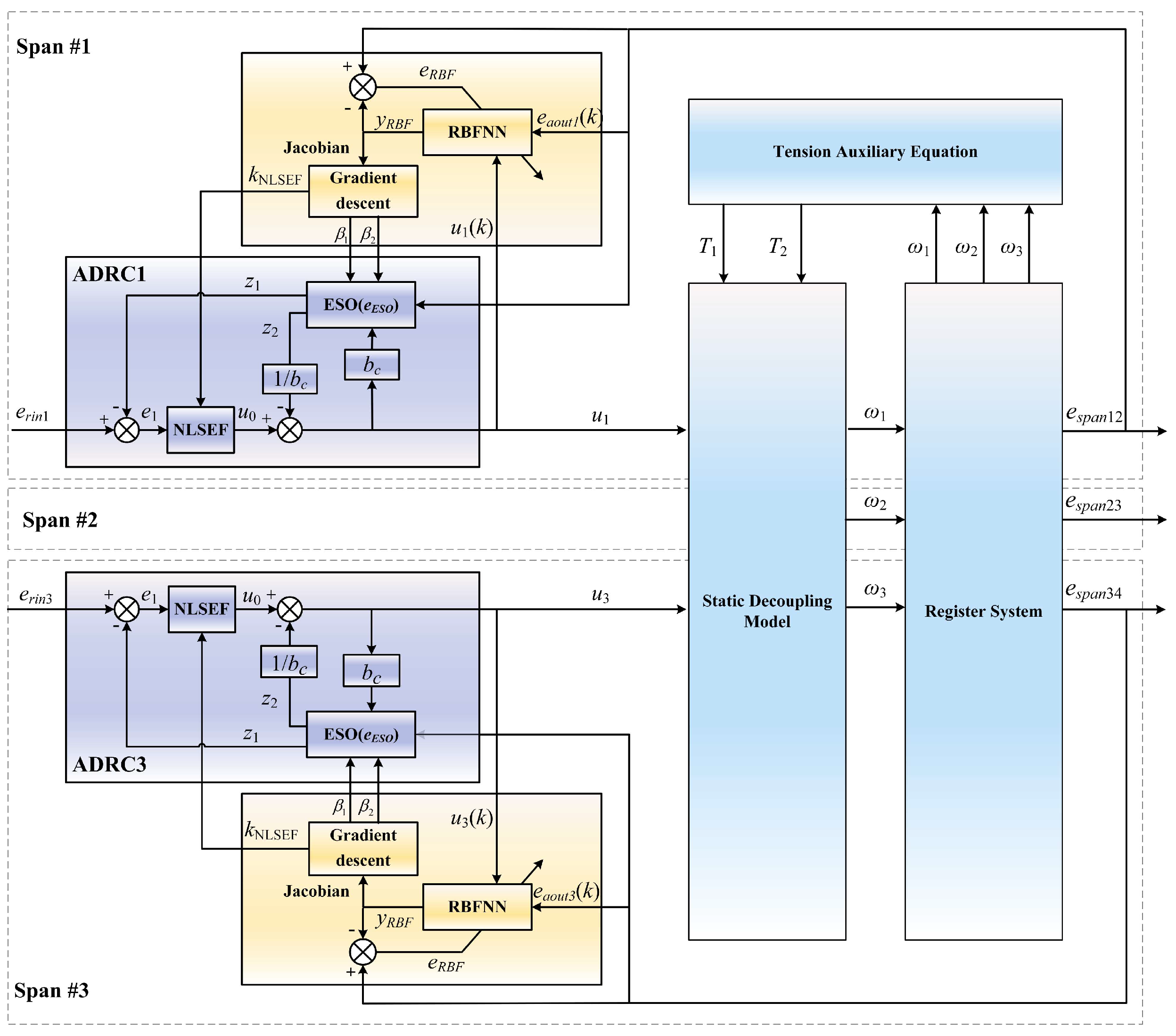
• Set the initial values of the RBF neural network parameters and the initial values of the ADRC controller parameters;
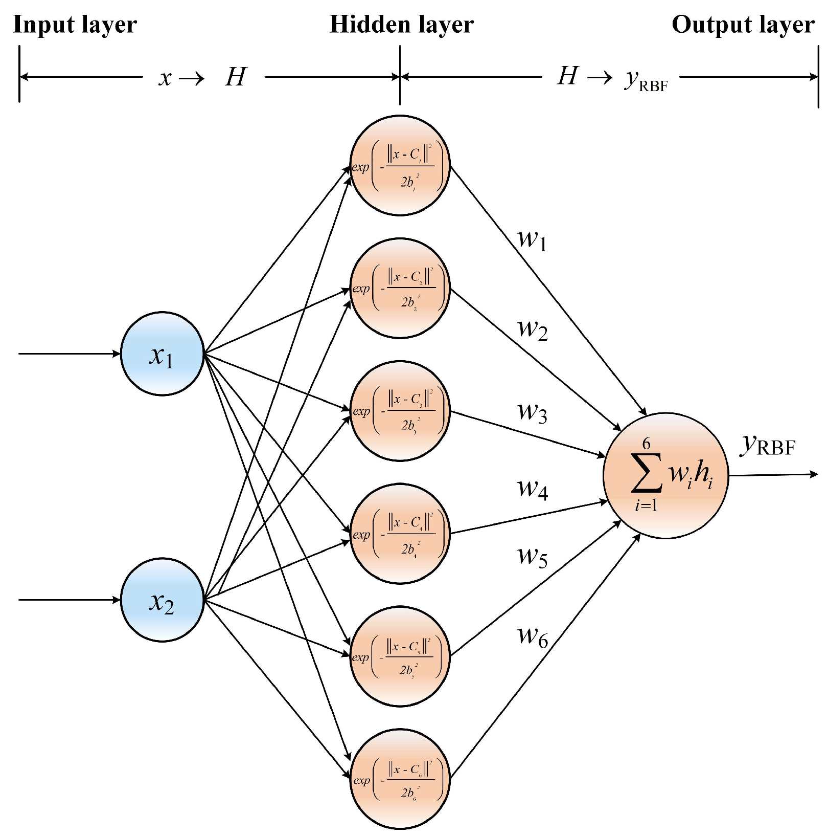
• The RBF neural network receives the output control signal u(k) from the ADRC controller and adjusts to the actual output error e_span(k) of the system;
• Calculate the identification model error metric e_RBF to update the RBF neural network parameters, including the center vector, basis width vector, and network weights; Then, calculate the system error metric E_control and, combined with the Jacobian information, update the ADRC controller parameters to correct β₁, β₂, k_NLSEF, and b_c;
• Judge whether the actual error e_span of the tuning system is within the acceptable range, and decide whether to proceed to the next cycle or to terminate.

4. Simulation and Analysis

The performance of the controller designed for the flexographic register system was verified by MATLAB 2019b, where the simulation parameters are the actual measured values of the actual flexographic press (made in Weinan KESAI, Weinan, China), as shown in Table 1. Simulation of the actual flexo printer in commissioning mode 50–100 m/min steady speed-acceleration-steady speed operation conditions (Trapezoid-variable acceleration, acceleration time 10 s), simulation substrate PET and BOPP film, simulation time 30 s, under different operating conditions (steady speed and acceleration cases), and the traditional PID controller and decoupling PID (structure as shown in Figure 9) are compared and verified, where the PID and the designed controller parameters are shown in

Table 2. Parameters of each RBF_ADRC controller.

Parameters	RBF_ADRC1	RBF_ADRC2	RBF_ADRC3
β1	5000	1800	20,100
β2	103,333	128,000	163,300
kNLSEF	150	410	130
δ	0.5	0.4	0.4
bc	1	1	1
η	0.25	0.42	0.45
η1	0.1	0.3	0.35
η2	0.02	0.035	0.035
η3	0.01	0.01	0.02
η4	0.002	0.001	0.003
α	0.5	0.5	0.5

and

Table 3. Parameters of each PID controller.

Parameters	PID1	PID2	PID3
kp	2.5	12	6
ki	5	20	2.7
kd	0	2	0

.

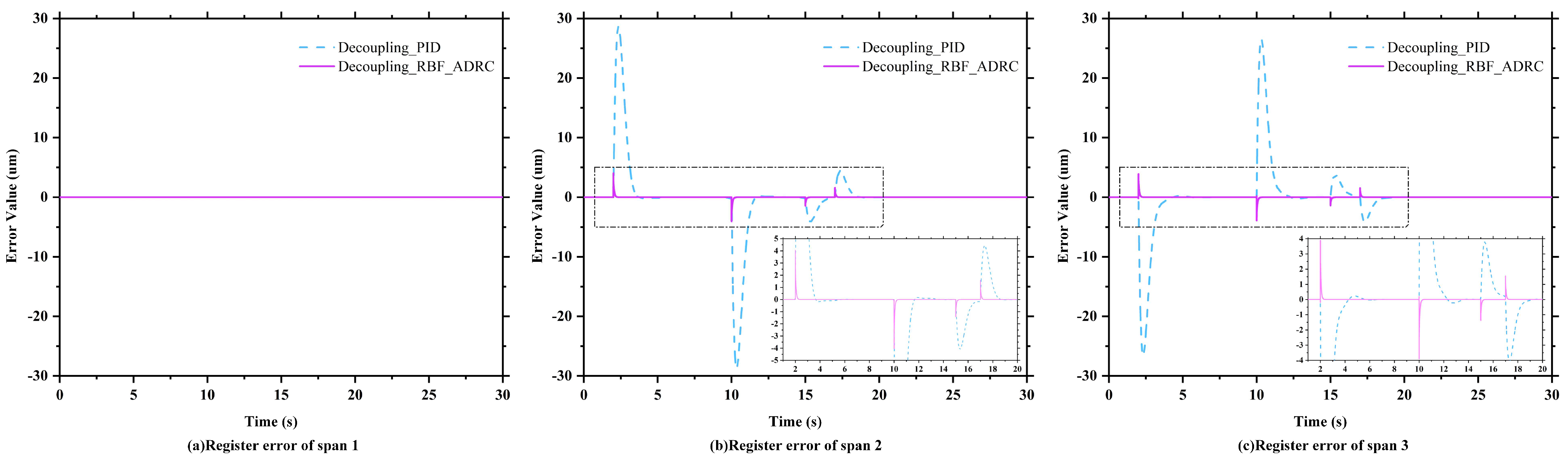
4.1. Verification of Decoupling Performance

It is verified that the latter register does not affect the former register by feeding a disturbance signal to the latter unit, and then the system is shown to be decoupled. The simulation conditions are as follows: under the 50 m/min steady speed stage, the tension is assumed to be stable at 100N, and after the stable operation of the system, ω₃ is allowed to produce an overshoot speed fluctuation with an amplitude of 0.25 m/min in the 2nd second, which lasts for 8 s and then recovers; under the 50–100 m/min trapezoidal variable acceleration stage (after the simulation time of 10 s), T₂ is allowed to produce a 10 N tension at the 15th second burst for 2 s. The static decoupled PID and static decoupled ADRC controller register error curves are shown in Figure 10.

Compared with Figure 10, under different controllers, both speed and tension fluctuations of this stage affect the latter register error, but have different decoupling abilities for the front register. Under PID control, fluctuations in ω₃ affect the front stage register e_span2, generating about ±30 μm error, but under the ADRC controller, fluctuations in ω₃ affect the front stage register e_span2, generating only ±4 μm fluctuations. Similarly, in the acceleration phase, T₂ generates tension fluctuations affecting e_span2 under PID control, which also generates a disturbance of about ±4.5 μm, but under ADRC control, the disturbance is only ±1 μm. This means that the ADRC controller involved has strong decoupling performance under speed disturbance or tension disturbance.

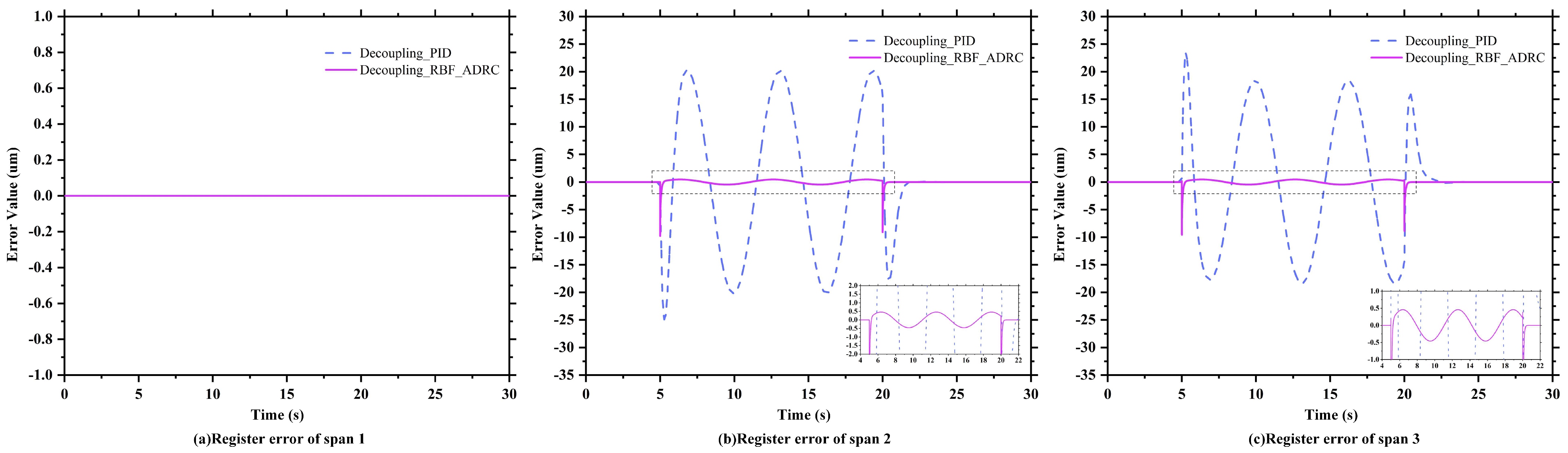
4.2. Verification of Robustness

To verify the internal robustness of the register system, the material properties of the strip (stretching characteristics of the same material at different temperatures, as well as at uniform temperatures of different materials) are used as internal disturbances. The simulation conditions are as follows: given T₁ at the 2nd second (steady state speed 50 m/min) with 10 N tension disturbance for 4 s and ω₁ at the 22nd second (steady state speed 100 m/min) with 0.5 m/min speed disturbance for 4 s, the system variable Young’s modulus E was changed with BOPP material at 10 °C (E = 2.60 Gpa), 20 °C (E = 2.24 Gpa), 30 °C (E = 2.02 Gpa), and Young’s modulus at 20 °C (E = 4.89 Gpa) for PET material for verification. The 3-span registration error curves of the conventional PID and the designed controller are shown in Figure 11.

Compared with Figure 11, the register error does not change with the change of Young’s modulus under the same speed perturbation, and the register error of 3-span under RBF_ADRC control is much smaller than the register error of PID control; under the same tension perturbation, the register error of 3-span under different controllers increases with the decrease in Young’s modulus, but the degree of decrease is not consistent. The peak of register error is smaller under the control of the designed controller, and the maximum is only ±3 μm, which proves its better robustness.

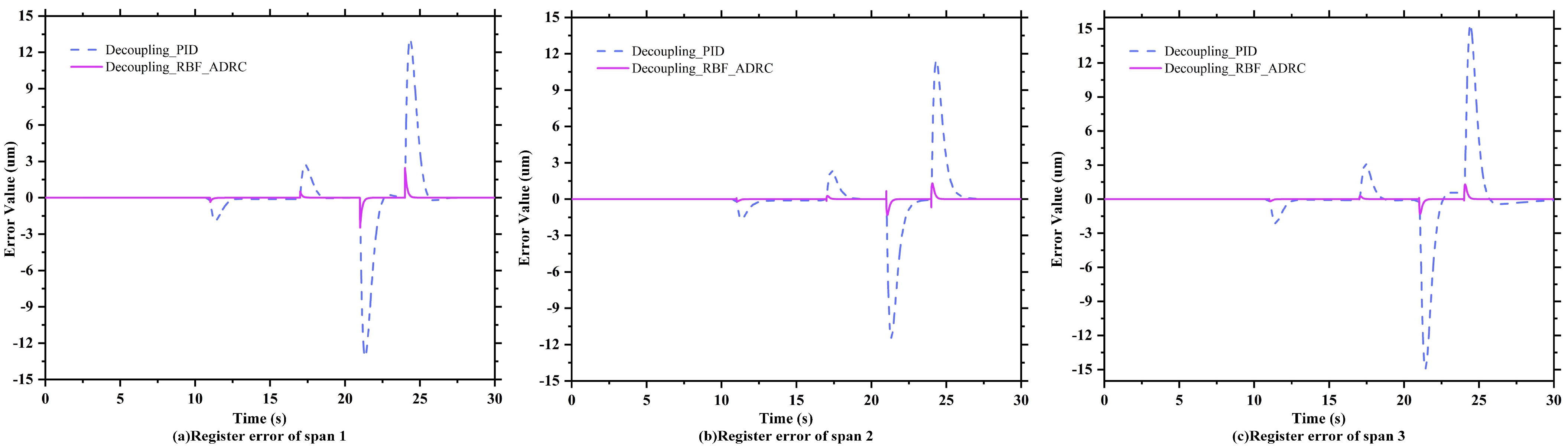
4.3. Verification of Anti-Interference Performance

The speed disturbance is easily generated during the operation of the equipment due to the non-rounding of the plate roller or electrical and mechanical reasons. To verify the speed disturbance performance of the controller, the speed fluctuation condition in the actual printing process is simulated, specifically: let ω₃ produce a sinusoidal overshoot speed fluctuation with an amplitude of 0.25 m/min (corresponding to the fixed period signal such as the plate roller is not round) in the 5th second (50 m/min steady state speed) for 15 s until the acceleration to 100 m/min. The decoupling PID and the designed controller register error curve are shown in Figure 12.

Compared with Figure 12, the speed fluctuation of ω₃ leads to different peak deviations of the span 2 and span 3 register errors e_span2 and e_span3 in different operation stages under different controllers. In the 50 m/min steady speed operation environment, the peak of the 3-span error reaches a maximum of ±23 μm when decoupled PID control, while the peak of the 3-span register error is only ±10 μm at the maximum when controlled by the designed controller, with a peak reduction of about 56% compared to the decoupled PID control. Under the acceleration condition from 50 to 100 m/min, the maximum peak 3-span error of the decoupled PID controller reaches ±18 μm, while the maximum peak 3-span register error of the designed controller is only ±0.5 μm. Therefore, the designed controller has good immunity to the errors caused by speed variations.

In addition, the steady-state tension may change during the material change process or the rotation of the flip frame, resulting in a backward propagating tension disturbance. Therefore, the tension fluctuation conditions in the actual printing process are simulated as follows: let the tension T₁ in the infeeding unit generate a tension pulse disturbance of 5 N for 6 s at the 11th second (in the acceleration stage), and then generate a tension disturbance of 20 N for 3 s at the 21st second (in the 100 m/min steady speed stage). The decoupled PID and the designed controller registration error curve are shown in Figure 13.

Compared with Figure 13, the register error generated by tension disturbance is not consistent with the error control effect under different controllers. Under the 5 N disturbance in the acceleration phase, the peak 3-span register errors are ±2.7 μm, ±2.4 μm, and ±3.1 μm under the decoupled PID control, and ±0.53 μm, ±0.3 μm, and ±0.28 μm under the designed controller control. It is clear that the designed controller has good immunity to the error caused by tension variations compared to the decoupled PID controller.

5. Conclusions and Discussion

For the characteristics of multiple input multiple output and multi-span coupling of flexographic printing 4-color register system, a decoupling control strategy based on ADRC and RBF neural network is proposed in this paper. Its unique feature is to design a decoupling controller that relies on little model information and variable working condition parameter rectification by integrating the ADRC technique and RBF neural network through the static decoupling model. Among them, the static decoupling realizes the system single-input single-output decoupling calculation, the ADRC technique dynamically estimates the total system disturbance, and the RBF realizes the real-time adjustment of the ADRC controller parameters. In the decoupling performance simulation, the controller designed in this paper reduces the maximum peak register error by 86.7% compared with the traditional PID controller. In the robustness simulation experiment, the maximum peak register error under the control of the controller designed in this paper is only 3 μm, which is 75% lower than that of the traditional PID. In the anti-jamming simulation experiment, the controller designed in this paper reduces the peak register error by 97.2%. The simulation results show that the decoupling performance, robustness and anti-interference capability of the designed controller are better compared with the PID-based controller under different working conditions (steady speed and acceleration), and the peak register error is significantly reduced (<±10 μm), which realizes the high accuracy control of the register system.

The ADRC control strategy based on the RBF neural network proposed in this paper shows superior decoupling performance, robustness, and anti-interference ability in simulations. In future work, the focus will be on analyzing the coupling interfaces of the actual anilox roller, coating roller, and bottom roller in flexographic printing machines and integrating the designed controller algorithm into existing industrial control systems. Meanwhile, with the rise of spiking neural networks and other neuromorphic systems, controllers combining PID controllers with neuromorphic systems have greatly enhanced control performance in fields such as robotics [21] and autonomous driving [22]. In future work, we will further validate the control performance of PID controllers integrated with neuromorphic systems in alignment systems. At the same time, neuromorphic electronic devices such as ion-gated vertical transistors, which offer numerous advantages like low power consumption, fast response, and multimodal integration [23], will be applied in print alignment error detection and control of servo drivers to further validate the control algorithm designed in this paper.

References

1. Huang, H.; Xu, J.; Sun, K. Design and Analysis of Tension Control System for Transformer Insulation Layer Winding. IEEE Access. 2020, 8, 95068–95081. [Google Scholar] [CrossRef]
2. Jabbar, K.A.; Pagilla, P.R. Modeling and Analysis of Web Span Tension Dynamics Considering Thermal and Viscoelastic Effects in Roll-to-Roll Manufacturing. J. Manuf. Sci. Eng. 2018, 140, 051005. [Google Scholar] [CrossRef]
3. Lee, J.; Jo, M.; Lee, C. Advanced Tension Model for Highly Integrated Flexible Electronics in Roll-To-Roll Manufacturing. IEEE/ASME Trans. Mechatron. 2021, 27, 2908–2917. [Google Scholar] [CrossRef]
4. Wang, Z.; Liu, S.; Feng, L. Coupling Modeling and Analysis of the Tension System for Roll-to-Roll Gravure Printing Machines. J. Imaging Sci. Technol. 2021, 66, 020401–02040110. [Google Scholar] [CrossRef]
5. Chen, Z.; Zheng, Y.; Zhang, T. Modeling and Register Control of the Speed-up Phase in Roll-to-Roll Printing Systems. IEEE Trans. Autom. Sci. Eng. 2018, 16, 1438–1449. [Google Scholar] [CrossRef]
6. Chen, Z.; Ying, Z.; Zhou, M. Model-Based Feedforward Register Control of Roll-to-Roll Web Printing Systems. Control. Eng. Pract. 2016, 51, 58–68. [Google Scholar] [CrossRef]
7. Chen, Z.; He, J.; Ying, Z. An Optimized Feedforward Decoupling PD Register Control Method of Roll-to-Roll Web Printing Systems. IEEE Trans. Autom. Sci. Eng. 2016, 13, 274–283. [Google Scholar] [CrossRef]
8. Chen, Z.; Zhang, T.; Zheng, Y. Fully Decoupled Control of the Machine Directional Register in Roll-to-Roll Printing System. IEEE Trans. Ind. Electron. 2020, 68, 10007–10018. [Google Scholar] [CrossRef]
9. Lee, J.; Shin, K.; Lee, C. Analysis of Dynamic Thermal Characteristic of Register of Roll-to-Roll Multi-Layer Printing Systems. Robot. Comput.-Integr. Manuf. 2015, 35, 77–83. [Google Scholar] [CrossRef]
10. Lee, J.; Seong, J.; Park, J. Register Control Algorithm for High Resolution Multilayer Printing in the Roll-to-Roll Process. Mech. Syst. Signal Process. 2015, 60, 706–714. [Google Scholar] [CrossRef]
11. Lee, J.; Shin, K.H.; Kang, H. Design of A Register Controller Considering Inherent Characteristics of a Roll-to-Roll Continuous Manufacturing System. Int. J. Adv. Manuf. Technol. 2019, 102, 3725–3737. [Google Scholar] [CrossRef]
12. Lee, J.; Shin, K.; Jung, H. Control Scheme for Rapidly Responding Register Controller Using Response Acceleration Input in Industrial Roll-To-Roll Manufacturing Systems. IEEE Trans. Ind. Electron. 2021, 69, 5215–5224. [Google Scholar] [CrossRef]
13. Kang, H.; Lee, C.; Shin, K. Modeling and Compensation of The Machine Directional Register in Roll-to-Roll Printing. Control Eng. Pract. 2013, 21, 645–654. [Google Scholar] [CrossRef]
14. Kim, C.; Jeon, S.W.; Kim, C.H. Reduction of Linearly Varying Term of Register Errors Using a Dancer System in Roll-to-Roll Printing Equipment for Printed Electronics. Int. J. Precis. Eng. Manuf. 2019, 20, 1485–1493. [Google Scholar] [CrossRef]
15. Jung, H.; Nguyen, A.D.; Choi, J. High-Precision Register Error Control Using Active-Motion-Based Roller in Roll-to-Roll Gravure Printing. Jpn. J. Appl. Phys. 2018, 57, 05GB04. [Google Scholar] [CrossRef]
16. Liu, S.; Mei, X.; Li, J. Design Feedforward Active Disturbance Rejection Control Controller for Multi-Color Register System. J. Mech. Eng. 2015, 51, 143–150. [Google Scholar] [CrossRef]
17. Li, M.; Feng, H.; Zhang, Y. RBF Neural Network Tuning PID Control Based on UMAC. J. Beijing Univ. Aeronaut. Astronaut. 2018, 44, 2063. [Google Scholar]
18. Kumar, R.; Agrawal, H.P.; Shah, A. Maximum Power Point Tracking in Wind Energy Conversion System Using Radial Basis Function Based Neural Network Control Strategy. Sustain. Energy Technol. Assess. 2019, 36, 100533. [Google Scholar] [CrossRef]
19. Guo, X.; Tan, A.; Wang, Q. Active disturbance rejection control with adaptive RBF neural network for a permanent magnet spherical motor. ISA Trans. 2025, 156, 678–688. [Google Scholar] [CrossRef] [PubMed]
20. Li, J.; Mei, X.S.; Tao, T. Research on the Register System Modeling and Control of Gravure Printing Press. J. Mech. Eng. Sci. 2012, 226, 626–635. [Google Scholar] [CrossRef]
21. Marrero, D.; Kern, J.; Urrea, C. A Novel Robotic Controller Using Neural Engineering Framework-Based Spiking Neural Networks. Sensors 2024, 24, 491. [Google Scholar] [CrossRef] [PubMed]
22. Halaly, R.; Elishai, E.T. Autonomous Driving Controllers with Neuromorphic Spiking Neural Networks. Front. Neurorobotics 2023, 17, 1234962. [Google Scholar] [CrossRef] [PubMed]
23. Merces, L. Advanced Neuromorphic Applications Enabled by Synaptic Ion-Gating Vertical Transistors. Adv. Sci. 2024, 11, 2305611. [Google Scholar] [CrossRef]
Figure 1. The physical structure of the inline flexographic printing machine.
Electronics 14 02162 g001
Figure 2. Simplified structure of the inline flexographic printing machine.
Electronics 14 02162 g002
Figure 3. Register system coupling interface.
Electronics 14 02162 g003
Figure 4. Register coupling interface without tension sensors.
Electronics 14 02162 g004
Figure 5. Multi-span register errors and tension fluctuation at different speeds.
Electronics 14 02162 g005
Figure 6. Multi-span register error and velocity fluctuation at different speeds.
Electronics 14 02162 g006
Figure 7. Structure of RBF_ADRC decoupling controller.
Electronics 14 02162 g007
Figure 8. The structure of the RBF neural network.
Electronics 14 02162 g008
Figure 9. The structure of the decoupled PID controller.
Electronics 14 02162 g009
Figure 10. Three-span decoupling register error curves.
Electronics 14 02162 g010
Figure 11. Three-span register error curves with different Young’s moduli.
Electronics 14 02162 g011
Figure 12. Three-span register error curves under velocity disturbance.
Electronics 14 02162 g012
Figure 13. Three-span register error curves under tension disturbance.
Electronics 14 02162 g013