
Overview and Comparison of Feedback-Based Dynamic Beam Focusing Techniques for Long-Range Wireless Power Transfer


Abstract
1. Introduction
2. Mathematical Framework to Analyze the Steady-State Efficiency of WPT
2.1. Notation
2.2. Preliminary System Setup
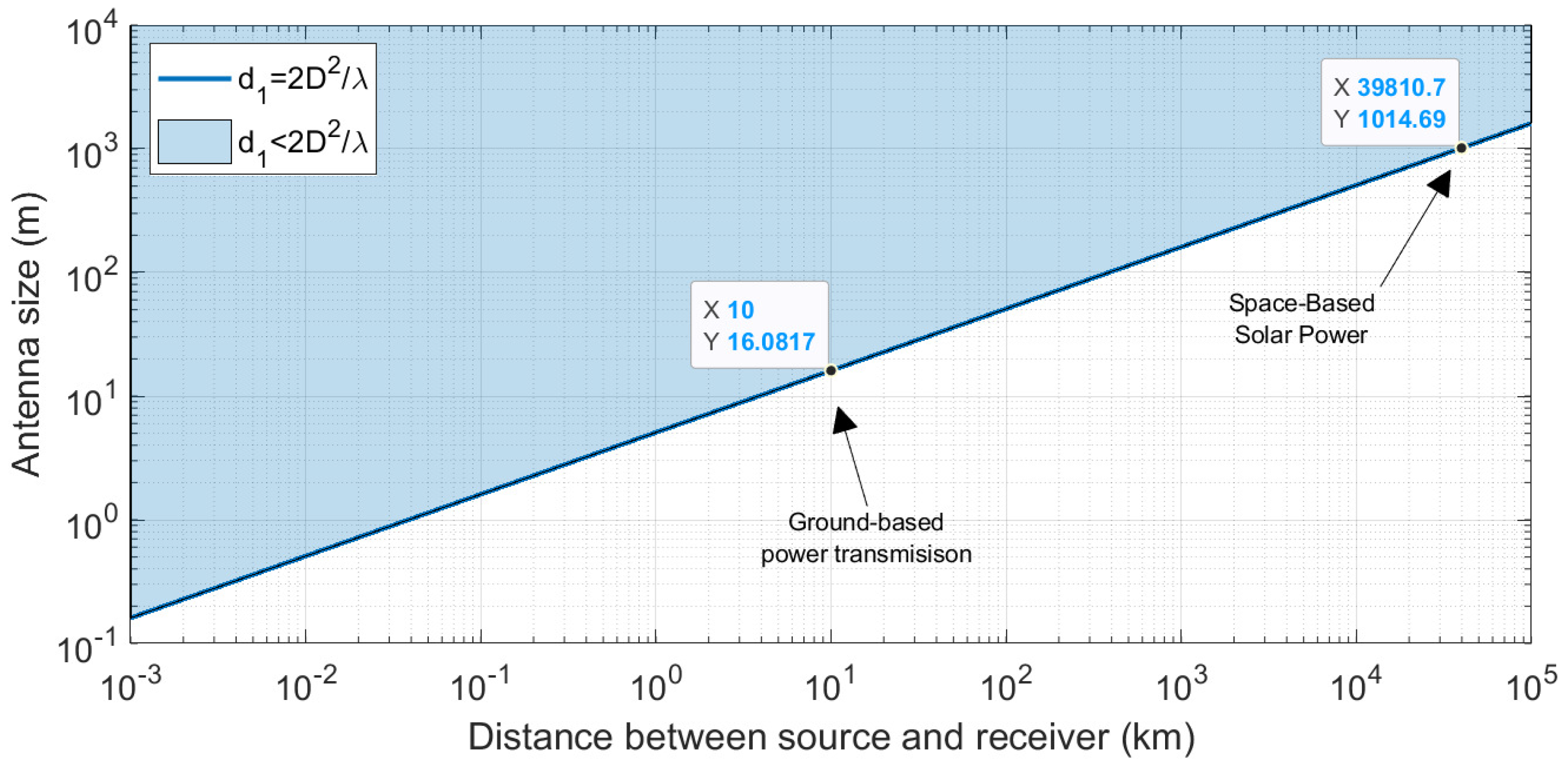
2.3. Maximum Theoretical WPT Efficiency
2.4. WPT Efficiency of Any Transmitter Input Configuration
3. Overview of Feedback-Based Dynamic Beam Focusing Techniques
3.1. Iterative Optimization Techniques
3.2. Techniques That Use Channel Estimation
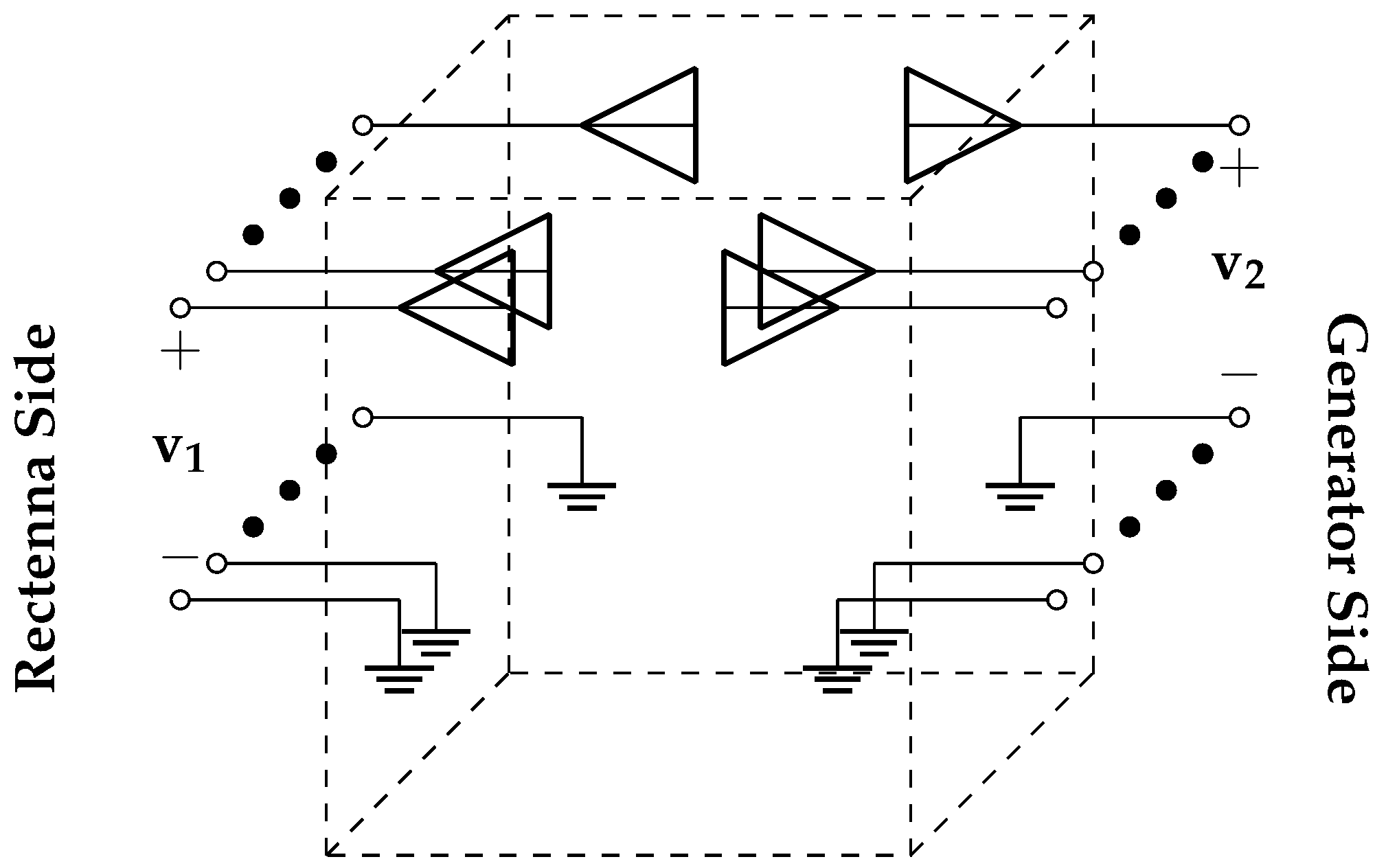
3.3. Both-Sides Retrodirective Beamforming System
3.4. Summary
4. Simulation and Comparison Methodology
4.1. Scope and Delimitations
4.2. Simulation Environments
4.2.1. One Transmitter to Two Receivers in Perfectly Absorbing Bounding Box
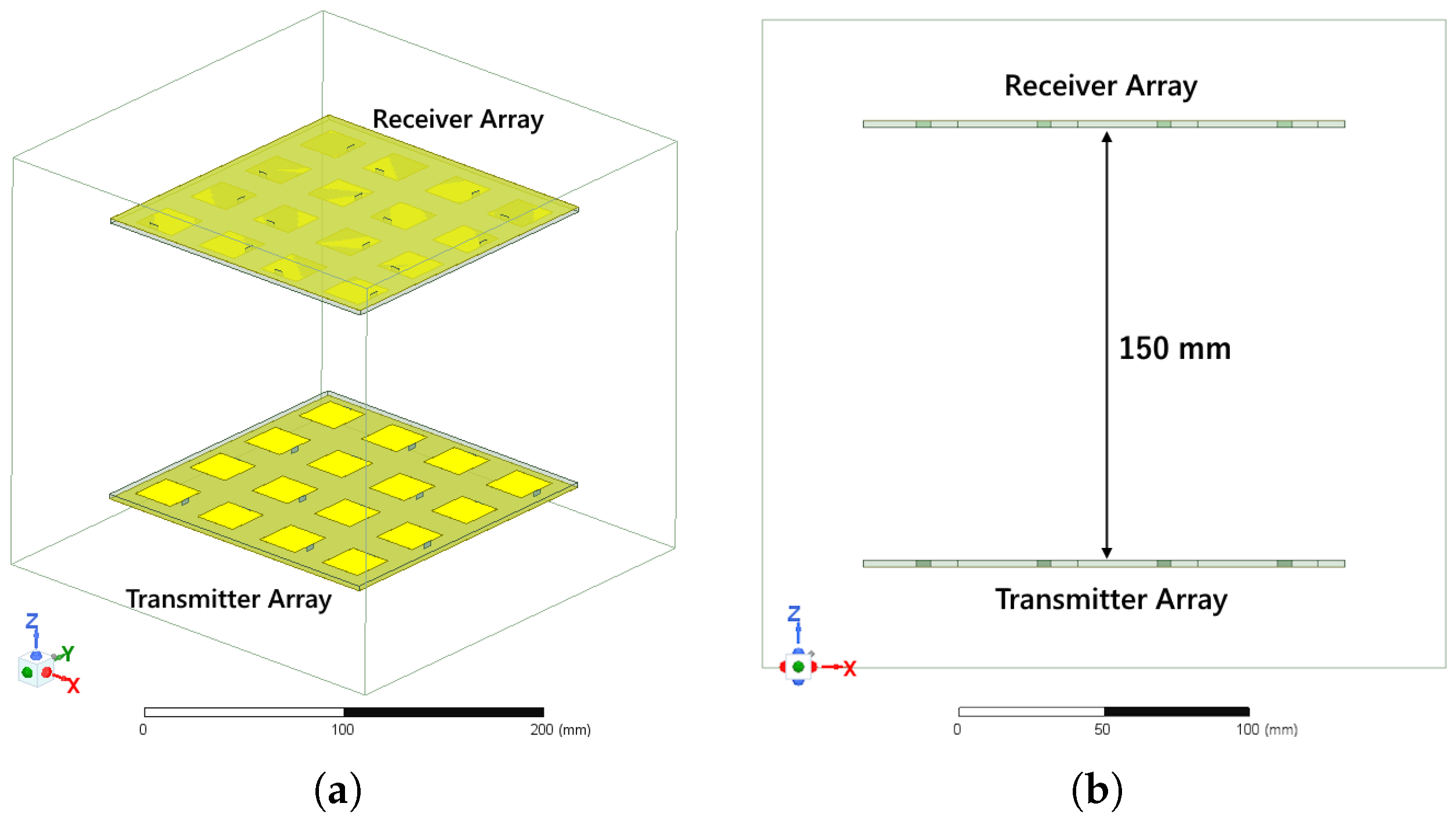
4.2.2. Sixteen-Element Transmitter and Receiver Planar Arrays in Absorbing Bounding Box
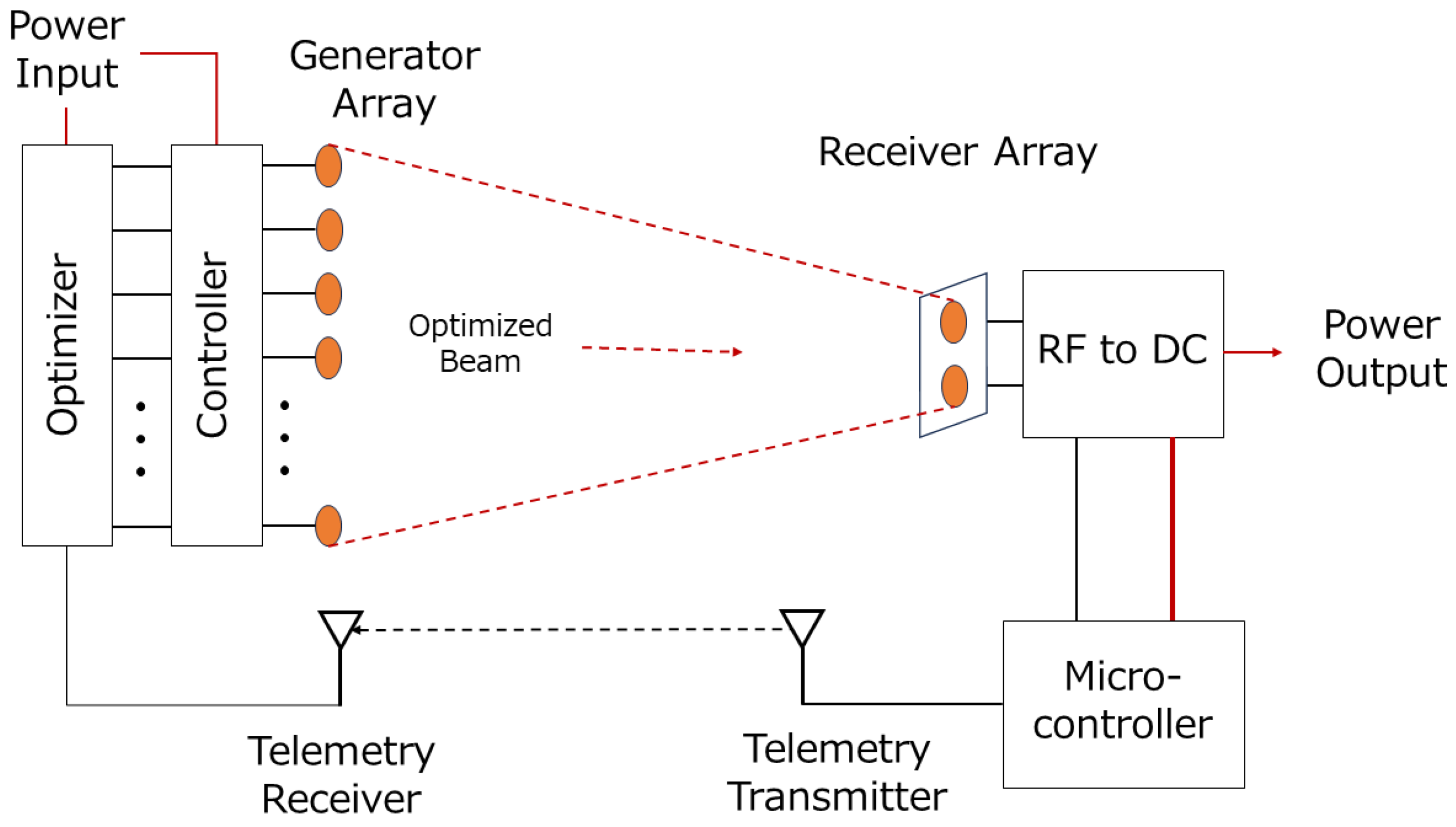
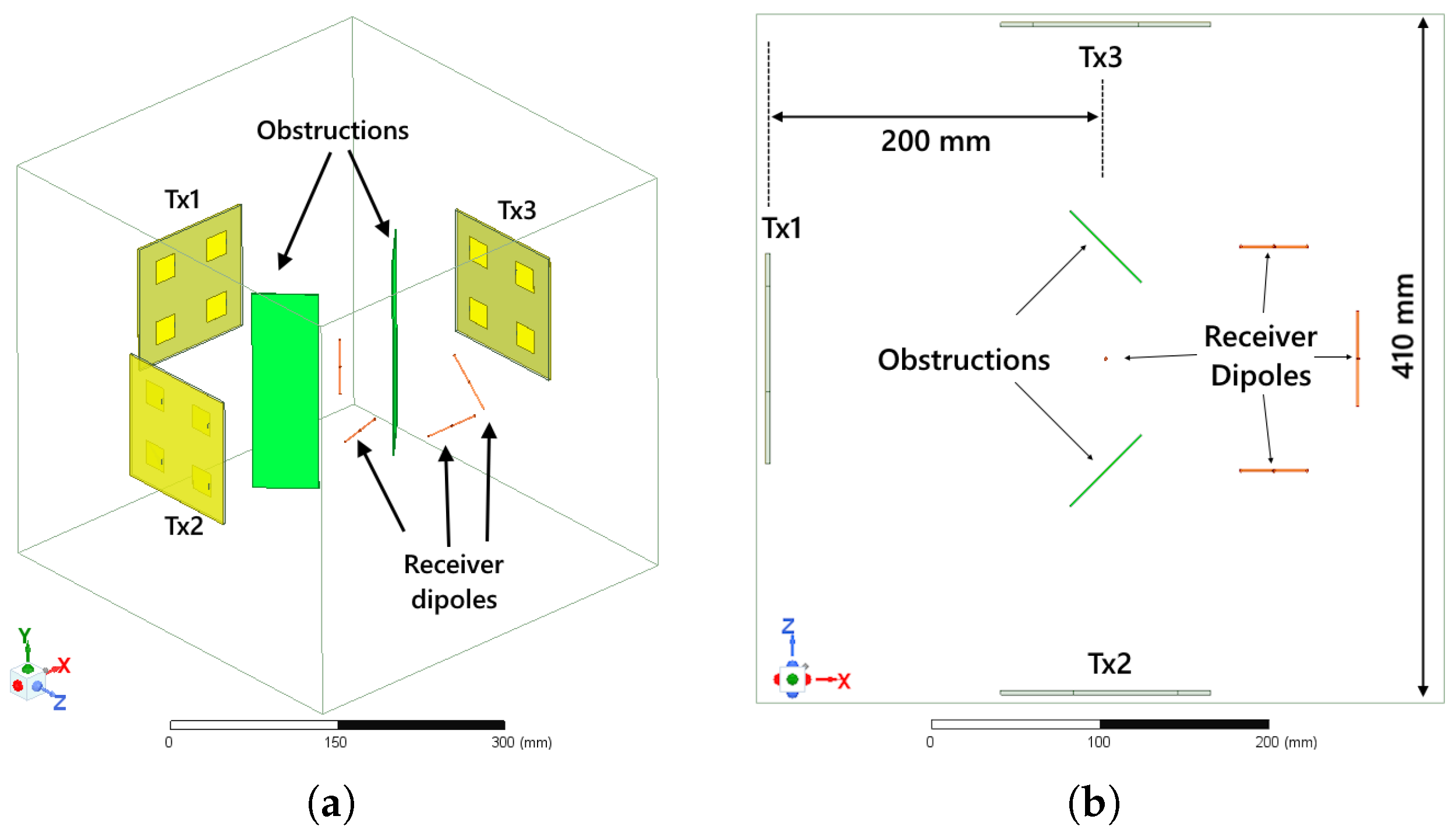
4.2.3. Distributed Transmitters to Multiple Receivers in a Partially Reflective Bounding Box
4.3. Comparison Metrics
4.3.1. Convergence Time
4.3.2. Steady-State Efficiency
4.4. Simulation Setup
4.4.1. Iterative Optimization Techniques
4.4.2. Techniques That Use Channel Estimation
4.4.3. Both-Sides Retrodirective Beamforming System
5. Results and Discussion
6. Conclusions
Funding
Data Availability Statement
Conflicts of Interest
References
- Pelham, T.; Chen, X.; Collins, B.; Parini, C.; Brown, A. An Overview of Gigascale Antenna Arrays and Electromagnetics for Space Based Solar Power. In Proceedings of the 2024 18th European Conference on Antennas and Propagation (EuCAP), Glasgow, UK, 17–22 March 2024; pp. 1–4. [Google Scholar] [CrossRef]
- Hajimiri, A.; Abiri, B.; Bohn, F.; Gal-Katziri, M.; Manohara, M.H. Dynamic Focusing of Large Arrays for Wireless Power Transfer and Beyond. IEEE J. Solid-State Circuits 2021, 56, 2077–2101. [Google Scholar] [CrossRef]
- Yang, B.; Mitani, T.; Shinohara, N. Auto-Tracking Wireless Power Transfer System With Focused-Beam Phased Array. IEEE Trans. Microw. Theory Tech. 2023, 71, 2299–2306. [Google Scholar] [CrossRef]
- Anselmi, N.; Tosi, L.; Rocca, P.; Toso, G.; Massa, A. A Self-Replicating Single-Shape Tiling Technique for the Design of Highly Modular Planar Phased Arrays—The Case of L-Shaped Rep-Tiles. IEEE Trans. Antennas Propag. 2023, 71, 3335–3348. [Google Scholar] [CrossRef]
- Hui, Q.; Jin, K.; Zhu, X. Directional Radiation Technique for Maximum Receiving Power in Microwave Power Transmission System. IEEE Trans. Ind. Electron. 2020, 67, 6376–6386. [Google Scholar] [CrossRef]
- Matsumuro, T.; Ishikawa, Y.; Mitani, T.; Shinohara, N.; Yanagase, M.; Matsunaga, M. Study of a single-frequency retrodirective system with a beam pilot signal using dual-mode dielectric resonator antenna elements. Wirel. Power Transf. 2017, 4, 132–145. [Google Scholar] [CrossRef]
- Koo, H.; Bae, J.; Choi, W.; Oh, H.; Lim, H.; Lee, J.; Song, C.; Lee, K.; Hwang, K.; Yang, Y. Retroreflective Transceiver Array Using a Novel Calibration Method Based on Optimum Phase Searching. IEEE Trans. Ind. Electron. 2021, 68, 2510–2520. [Google Scholar] [CrossRef]
- Choi, K.W.; Kim, D.I.; Chung, M.Y. Received Power-Based Channel Estimation for Energy Beamforming in Multiple-Antenna RF Energy Transfer System. IEEE Trans. Signal Process. 2017, 65, 1461–1476. [Google Scholar] [CrossRef]
- Miyamoto, R.; Itoh, T. Retrodirective arrays for wireless communications. IEEE Microw. Mag. 2002, 3, 71–79. [Google Scholar] [CrossRef]
- DiDomenico, L.; Rebeiz, G. Digital communications using self-phased arrays. IEEE Trans. Microw. Theory Tech. 2001, 49, 677–684. [Google Scholar] [CrossRef]
- Li, B.; Liu, S.; Zhang, H.L.; Hu, B.J.; Zhao, D.; Huang, Y. Wireless Power Transfer Based on Microwaves and Time Reversal for Indoor Environments. IEEE Access 2019, 7, 114897–114908. [Google Scholar] [CrossRef]
- Cangialosi, F.; Grover, T.; Healey, P.; Furman, T.; Simon, A.; Anlage, S.M. Time reversed electromagnetic wave propagation as a novel method of wireless power transfer. In Proceedings of the 2016 IEEE Wireless Power Transfer Conference (WPTC), Aveiro, Portugal, 5–6 May 2016; pp. 1–4. [Google Scholar] [CrossRef]
- Yuan, Q. S-Parameters for Calculating the Maximum Efficiency of a MIMO-WPT System: Applicable to Near/Far Field Coupling, Capacitive/Magnetic Coupling. IEEE Microw. Mag. 2023, 24, 40–48. [Google Scholar] [CrossRef]
- Oliveri, G.; Poli, L.; Massa, A. Maximum Efficiency Beam Synthesis of Radiating Planar Arrays for Wireless Power Transmission. IEEE Trans. Antennas Propag. 2013, 61, 2490–2499. [Google Scholar] [CrossRef]
- Yedavalli, P.S.; Riihonen, T.; Wang, X.; Rabaey, J.M. Far-Field RF Wireless Power Transfer with Blind Adaptive Beamforming for Internet of Things Devices. IEEE Access 2017, 5, 1743–1752. [Google Scholar] [CrossRef]
- Wu, J.; Yuan, Q.; Okada, T.; Yang, B. An estimation method of the 4-port S-parameters used for the E-MIMO approach. Space Sol. Power Wirel. Transm. 2024, 1, 148–151. [Google Scholar] [CrossRef]
- Matsumuro, T.; Ishikawa, Y.; Shinohara, N. Basic study of both-sides retrodirective system for minimizing the leak energy in microwave power transmission. IEICE Trans. Electron. 2019, 102, 659–665. [Google Scholar] [CrossRef]
- Xiong, M.; Liu, Q.; Wang, G.; Giannakis, G.B.; Huang, C. Resonant Beam Communications: Principles and Designs. IEEE Commun. Mag. 2019, 57, 34–39. [Google Scholar] [CrossRef]
- Ku, M.L.; Han, Y.; Lai, H.Q.; Chen, Y.; Liu, K.J.R. Power Waveforming: Wireless Power Transfer Beyond Time Reversal. IEEE Trans. Signal Process. 2016, 64, 5819–5834. [Google Scholar] [CrossRef]
- Ambatali, C.D.M.; Nakasuka, S. Characterizing the Dynamic Behavior of a Both-Sides Retrodirective System for the Control of Microwave Wireless Power Transfer. In Proceedings of the 2024 SICE International Symposium on Control Systems (SICE ISCS), Kochi, Japan, 27–30 August 2024; pp. 99–106. [Google Scholar] [CrossRef]
- Ambatali, C.D.; Nakasuka, S.; Yang, B.; Shinohara, N. Analysis and experimental validation of the WPT efficiency of the both-sides retrodirective system. Space Sol. Power Wirel. Transm. 2024, 1, 48–60. [Google Scholar] [CrossRef]
- Bae, J.; Yi, S.H.; Koo, H.; Oh, S.; Oh, H.; Choi, W.; Shin, J.; Song, C.M.; Hwang, K.C.; Lee, K.Y.; et al. LUT-Based Focal Beamforming System Using 2-D Adaptive Sequential Searching Algorithm for Microwave Power Transfer. IEEE Access 2020, 8, 196024–196033. [Google Scholar] [CrossRef]
- Han, Y.; Jin, S.; Wen, C.K.; Ma, X. Channel Estimation for Extremely Large-Scale Massive MIMO Systems. IEEE Wirel. Commun. Lett. 2020, 9, 633–637. [Google Scholar] [CrossRef]
- Kato, H.; Yuan, Q. Array Factor, Retrodirective, and E-MIMO Beamforming Technologies. In Proceedings of the 2023 IEEE International Symposium On Antennas And Propagation (ISAP), Kuala Lumpur, Malaysia, 30 October–2 November 2023; pp. 1–2. [Google Scholar] [CrossRef]
- Abeywickrama, S.; Samarasinghe, T.; Ho, C.K.; Yuen, C. Wireless Energy Beamforming Using Received Signal Strength Indicator Feedback. IEEE Trans. Signal Process. 2018, 66, 224–235. [Google Scholar] [CrossRef]
- Gowda, V.R.; Yurduseven, O.; Lipworth, G.; Zupan, T.; Reynolds, M.S.; Smith, D.R. Wireless Power Transfer in the Radiative Near Field. IEEE Antennas Wirel. Propag. Lett. 2016, 15, 1865–1868. [Google Scholar]
- Nelder, J.A.; Mead, R. A Simplex Method for Function Minimization. Comput. J. 1965, 7, 308–313. [Google Scholar] [CrossRef]


| Description | Type | Advantages | Disadvantages |
|---|---|---|---|
| Orthogonal phase masks with phase sweeping [2] | Iterative optimization type |
|
|
| Directional radiation with iterative iteration or DRIS [5] | Iterative optimization type |
|
|
| Directional radiation with area scanning or DRAS [5] Use of look-up table [22] | Iterative optimization type |
|
|
| Channel estimation using least square error (LSE) method [8,25] | Channel estimation type |
|
|
| Channel estimation using Kalman Filter (KF) [8] | Channel estimation type |
|
|
| Both-sides retrodirective antenna array [17] |
|
| |
| Method | Case 1 | Case 2 | Case 3 |
|---|---|---|---|
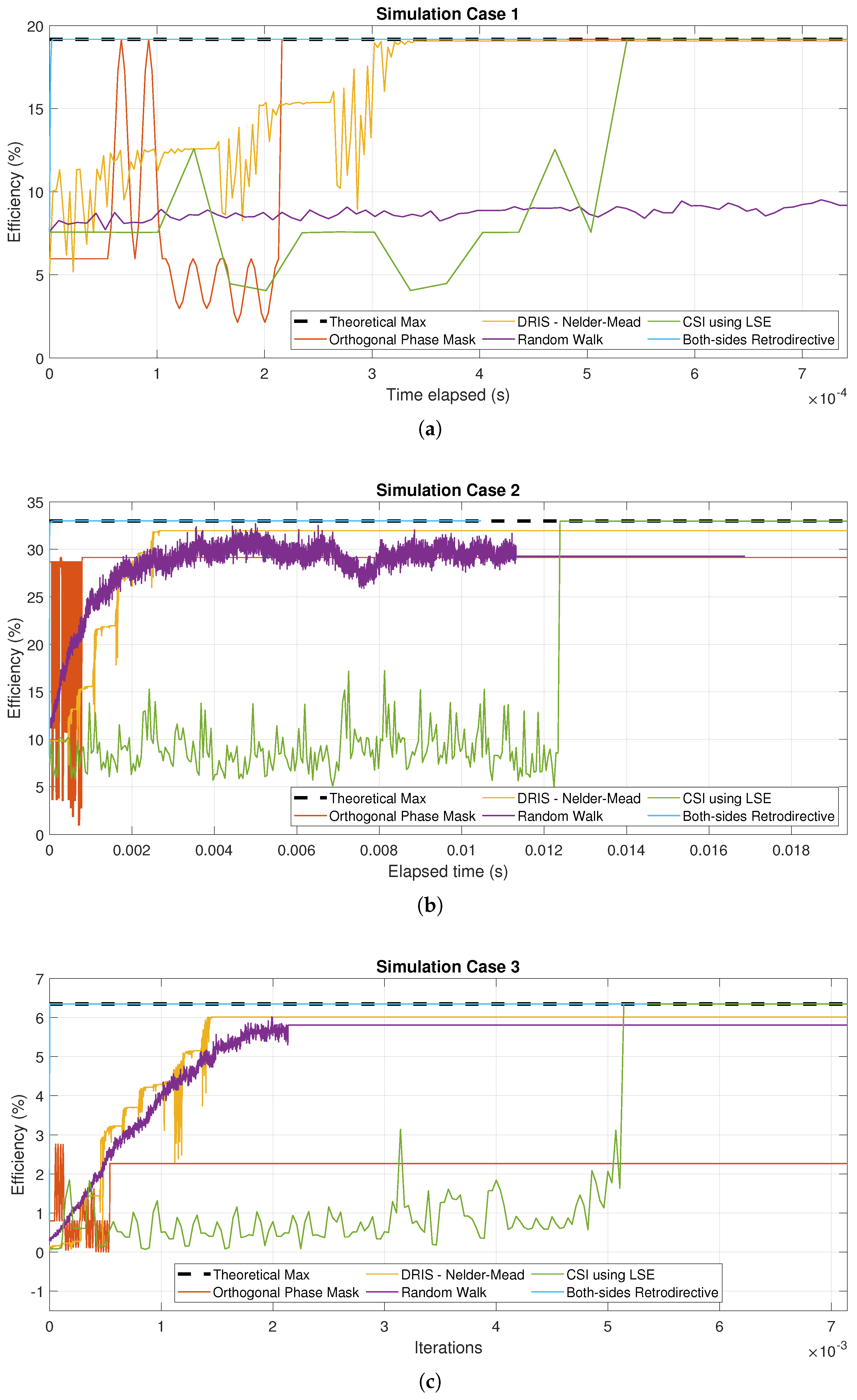
| = 19.17% | = 32.99% | = 6.35% | |
| Orthogonal Phase Mask [2] | 68 iterations | 272 iterations | 204 iterations |
| DRIS—Nelder–Mead [5] | 116 iterations | 1214 iterations | 606 iterations |
| Random Walk [15] | 3330 iterations | 6710 iterations | 1260 iterations |
| CSI estimation using LSE [8] | 17 iterations | 257 iterations | 145 iterations |
| Both-Sides Retrodirective System [17] | 5 iterations | 87 iterations | 5 iterations |
Disclaimer/Publisher’s Note: The statements, opinions and data contained in all publications are solely those of the individual author(s) and contributor(s) and not of MDPI and/or the editor(s). MDPI and/or the editor(s) disclaim responsibility for any injury to people or property resulting from any ideas, methods, instructions or products referred to in the content. |
© 2025 by the author. Licensee MDPI, Basel, Switzerland. This article is an open access article distributed under the terms and conditions of the Creative Commons Attribution (CC BY) license (https://creativecommons.org/licenses/by/4.0/).
Share and Cite
Ambatali, C.D. Overview and Comparison of Feedback-Based Dynamic Beam Focusing Techniques for Long-Range Wireless Power Transfer. Electronics 2025, 14, 2155. https://doi.org/10.3390/electronics14112155
Ambatali CD. Overview and Comparison of Feedback-Based Dynamic Beam Focusing Techniques for Long-Range Wireless Power Transfer. Electronics. 2025; 14(11):2155. https://doi.org/10.3390/electronics14112155
Chicago/Turabian StyleAmbatali, Charleston Dale. 2025. "Overview and Comparison of Feedback-Based Dynamic Beam Focusing Techniques for Long-Range Wireless Power Transfer" Electronics 14, no. 11: 2155. https://doi.org/10.3390/electronics14112155
APA StyleAmbatali, C. D. (2025). Overview and Comparison of Feedback-Based Dynamic Beam Focusing Techniques for Long-Range Wireless Power Transfer. Electronics, 14(11), 2155. https://doi.org/10.3390/electronics14112155