A Combined Detection Method for AC Fault Arcs Based on RLMD Decomposition and Pulse Density

Abstract

Despite the proliferation of methods for detecting AC arc faults, current solutions often fall short in balancing cost efficiency, real-time performance, and implementation flexibility. This paper proposes a novel joint detection method based on robust local mean decomposition (RLMD) and pulse density analysis. The method leverages a dual-path analog signal processing framework: the low-frequency component of the current transformer (CT) signal is digitized and decomposed using RLMD to extract statistical feature indicators, while the high-frequency component is fed into a high-speed comparator to generate TTL pulses, from which the pulse density is calculated within a sliding time window. By combining the characteristic quantities derived from RLMD with the temporal pulse density, the proposed scheme achieves accurate and efficient detection of arc faults. Experimental results validate the approach, demonstrating high detection probability, adjustable sensitivity, low power consumption, and cost-effectiveness. These attributes underscore the method’s practical relevance and engineering significance in intelligent fault monitoring systems.

1. Introduction

Low-voltage fault arcs represent a prevalent failure phenomenon in electrical equipment, attributed to various factors including loose contacts, insulation degradation, animal gnawing, and mechanical stress. These conditions are significant contributors to the occurrence of electrical fires. In response to the serious hazards associated with arc faults, relevant standards have been established both domestically and internationally. In 2008, the United States issued the UL 1699 standard, while the International Electrotechnical Commission (IEC) promulgated the IEC 62606:2013 [1] standard. In China, the national standard titled “General Requirements for Arc Fault Detection Devices (AFDD)” has been released, along with two product standards: GB 14287.4-2014 [2] and GB/T 31143-2014 [3]. These standards delineate the application requirements for fault arc detection with a rated voltage not exceeding 240 V and a rated current not exceeding 63 A.

In the context of the extensive demand for fault arc detection, the diversity of fault arc types necessitates the development of an engineering solution characterized by real-time performance, low cost, and high flexibility. Typical methods for detecting fault arcs primarily include time-domain methods [4], frequency-domain methods [5], transform-domain methods [6], and recognition methods based on machine learning and neural networks [7].

The time-domain method detects faults through statistical features such as standard deviation, kurtosis, and RMS. Artale et al. [4] analyzed the sensitivity of these parameters under various noise levels and threshold conditions. Li et al. [8] combined time–frequency features with a random forest algorithm to achieve a 100% recognition rate. Ratnakar et al. [9] proposed a rapid detection method based on statistical parameters. Seo et al. [10] achieved 99.999% accuracy in DC microgrids, significantly reducing false alarms. Atharparvez et al. [11] developed an effective algorithm to distinguish low-current faults. However, this method suffers from large errors, inflexible parameter tuning, and a high false alarm rate.

The frequency-domain method extracts features using FFT, CZT, or impedance modeling. Hwang et al. [5] proposed a wind power system fault detection method that does not require external devices. Balamurugan et al. [12] used FFT and STFT to detect arc faults in photovoltaic systems, meeting UL1699B standards. Artale et al. [13] employed CZT for high-resolution harmonic analysis to differentiate arcing from non-arcing states. He et al. [14] applied wavelet transform as a preprocessing step to improve detection accuracy. Park et al. [15] and Nutenki et al. [16] proposed detection algorithms based on current fluctuations and Mel-frequency cepstral coefficients (MFCC), respectively.

Transform-domain methods rely on wavelet transform, EMD, and VMD. Dang et al. [17] combined current signal analysis with machine learning models to detect parallel arc faults. Anggriawan et al. [18] achieved 99.97% detection accuracy by integrating continuous wavelet transform with neural networks. Miao et al. [19] and Duan et al. [20] used modified EMD and CNN to achieve high-precision detection without predefined thresholds. Zhao et al. [21] proposed an optimized VMD and least squares support vector machine (SVM) method, achieving recognition rates over 97%.

AI-based methods have shown exceptional performance in improving arc fault detection accuracy. Z. Li et al. [7] explored the potential of AI technologies such as electromagnetic radiation and arc sound for photovoltaic systems. Anggriawan et al. [18] maintained high accuracy under voltage fluctuations using continuous wavelet transform and neural networks. Le et al. [22] applied ensemble learning for detecting DC arcs across different loads. Z. He et al. [23] combined load classification with CNN, achieving accuracies over 95%. Miao et al. [19] improved performance by integrating EMD with SVM. However, AI methods require substantial hardware resources, extensive training time, and high-quality sample datasets, leading to higher training costs and large storage demands.

Although existing methods have achieved satisfactory detection accuracy, several limitations remain: time-domain approaches often suffer from high false alarm rates and inflexible parameter tuning; frequency-domain and transform-domain methods entail high computational costs and poor real-time performance; and AI-based techniques rely heavily on large datasets and high-end hardware, resulting in substantial training and implementation costs. To address the three key challenges of low cost, high real-time performance, and strong system flexibility, this study proposes a novel arc fault detection algorithm that combines time-domain pulse density analysis with low-frequency RLMD decomposition. An engineering-oriented detection system is designed and implemented, employing operational amplifiers, comparators, and a high-speed microcontroller unit (MCU), thereby avoiding the use of expensive high-precision ADCs and FPGAs. The system achieves low-latency analog filtering and pulse extraction, while RLMD requires minimal computational resources. Furthermore, it supports multi-threshold settings and integrates real-time and statistical feature parameters for robust decision-making. Experimental results demonstrate that the proposed method achieves high detection accuracy and a low false alarm rate, and the effectiveness of the approach has been validated through a functional engineering prototype.

The Section 1 of this paper introduces the application background, reviews relevant literature, outlines the research objectives, and presents the overall organization of the manuscript. The Section 2 provides an overview of the mathematical modeling of arc faults, along with the principles and implementation of the RLMD-based detection algorithm. The Section 3 describes the overall design and implementation of the proposed system, encompassing both hardware and software components. The Section 4 details the experimental platform and presents a comprehensive analysis and validation of the proposed method. Finally, the Section 5 concludes the study and offers perspectives for future research.

2. Arc Model and Detection Algorithm

2.1. Fault Arc Model

The mathematical models for fault arcs primarily include the Cassie arc model and the Mayr arc model, with the Mayr arc model demonstrating relatively higher accuracy.

The assumptions of the Cassie arc model are as follows: the arc channel is cylindrical, with the diameter of the arc column varying in accordance with the current; the voltage gradient across the arc remains constant; the temperature of the arc is uniformly distributed across the cross-section and remains constant in both time and space; and the rate of energy dissipation from the arc is proportional to the changing cross-section of the arc column. The differential equation governing the Cassie arc model is expressed as follows:

$${\displaystyle \frac{1}{g_a}}{\displaystyle \frac{d}{dt}}\left(g_a\right)={\displaystyle \frac{1}{v_c}}\left({\displaystyle \frac{E^2}{E_0^2}}-1\right)$$

(1)

$$v_c={\displaystyle \frac{q_c}{p_c}}$$

(2)

In the equation, $g_a$ represents the instantaneous value of the unit length arc conductivity, $v_c$ denotes the time constant of the Cassie arc model, $q_c$ is the energy constant per unit volume within the arc, $P_c$ refers to the power dissipation constant per unit volume of the arc, $E$ is the instantaneous value of the arc column voltage gradient, and $E_0=\sqrt{R_c{P}_c}$ is the static arc voltage gradient constant, where $R_c$ is the resistance constant per unit volume of the arc.

Mayr proposed the dynamic equation for the arc as follows:

$${\displaystyle \frac{1}{g_a}}{\displaystyle \frac{d}{dt}}\left(g_a\right)={\displaystyle \frac{1}{v_M}}\left({\displaystyle \frac{P}{P_a}}-1\right)$$

(3)

$$v_M={\displaystyle \frac{Q_a}{p_a}}$$

(4)

In the equation, $g_a$ represents the instantaneous value of the unit length arc conductivity, $v_M$ denotes the time required for the change in energy within the arc gap to result in a change in arc gap resistance by a factor of $e$, $Q_a$ is the energy required for the arc current to change by a factor of $e$, $P$ is the instantaneous value of the input power per unit length of the arc, and $P_a=E{i}_a$ is the power dissipation constant per unit length of the arc, where $i_a$ is the instantaneous value of the arc current.

Both arc models represent simplified abstractions of real physical phenomena, with the common primary variable being the instantaneous value of conductivity. The arc can be conceptualized as a rapidly changing dynamic resistor. Testing conducted on arc platforms and equivalent calculations indicate that the variation range in arc resistance is approximately on the order of several to hundreds of milliohms. Frequency-domain measurements reveal that the predominant frequency components of most fault arcs fall within the range of 100 kHz to 300 kHz. Among these, the Mayr arc model aligns more closely with the measured values.

2.2. RLMD Signal Decomposition Algorithm

The robust local mean decomposition (RLMD) algorithm is an improved version of the local mean decomposition (LMD) method, designed to address the limitations of LMD in terms of its sensitivity to noise and outliers. LMD, proposed by Smith, is an adaptive signal processing technique whose core idea lies in iteratively separating the local mean and envelope of a signal. The original signal is thereby decomposed into a sum of several product function (PF) components and a residual. Each PF is composed of an envelope function and a corresponding purely frequency-modulated (FM) signal. However, the traditional LMD algorithm suffers from issues such as end effects and mode mixing. RLMD enhances the computation of local statistical measures and smoothing strategies employed in conventional LMD, enabling stable decomposition of noisy signals and improving the overall robustness of the signal decomposition process.

The specific process of RLMD algorithm [24] is as follows:

• Boundary processing and extremum extraction: The signal $x(n)$ is extended at both ends using a mirror extension algorithm, after which all local extrema points $n_k(k=1,2,\dots )$ are identified.
• Local feature computation: Based on the adjacent extrema points $n_k$ and $n_{k+1}$, the local mean $m_k$ and local amplitude $a_k$ are calculated.

  $$m_k={\displaystyle \frac{n_k+n_{k+1}}{2}}$$

  (5)

  $$a_k={\displaystyle \frac{|n_k-n_{k+1}|}{2}}$$

  (6)
• Adaptive envelope estimation: $m_k$ and $a_k$ are processed using a moving average algorithm to generate a smoothed local mean function $m(n)$ and a local envelope function $a(n)$, and statistical methods are used to determine the optimal subset size ${\lambda }^{\ast }$.

  $$\mu s={\displaystyle \sum _{i=1}^{K-1}s(i)f(i)}$$

  (7)

  $$\delta s=\sqrt{{\displaystyle \sum _{i=1}^{K-1}{[s(i)-\mu s]}^2\cdot f(i)}}$$

  (8)

  $${\lambda }^{*}=odd(\mu s+3\ast \delta s)$$

  (9)

  where $s(i)$ denotes the step size for $m_k$ and $a_k$. $\mu s$ represents the mean of step size, and $\delta s$ denotes the standard deviation of step size. $f(i)$ is the probability of each interval. The $odd()$ function takes the nearest odd integer.
• Signal demodulation iteration: Firstly, $m_{11}(n)$ is separated from the original signal $x(n)$ to obtain the estimated zero mean signal $h_{11}(n)$. Secondly, the signal $h_{11}(n)$ is demodulated using $a_{11}(n)$ to obtain an estimated frequency modulation signal $s_{11}(n)$. The index $m_{ij}(n)$, $a_{ij}(n)$, $h_{ij}(n)$, $s_{ij}(n)$ represents the i-th PF component and j-th filtering process. The expression is:

  $$h_{11}(n)=x(n)-m_{11}(n)$$

  (10)

  $$s_{11}(n)={\displaystyle \frac{h_{11}(n)}{a_{11}(n)}}$$

  (11)

Construct a dual criterion objective function: When $f_{1j+1}>f_{1j}$ and $f_{ij+2}>f_{ij+1}$ are satisfied for three consecutive iterations, the screening stops and the result of the j − 1 th iteration is returned; Otherwise, the filtering process continues until the maximum number of iterations is reached. The objective function $f$ is defined as follows:

$$z(n)=a(n)-1$$

(12)

$$f=RMS[z(n)]+EK[z(n)]$$

(13)

$$RMS(z(n))=\sqrt{{\displaystyle \frac{1}{N_s}}{\displaystyle \sum _{n=1}^{N_s}{(z(n))}^2}}$$

(14)

$$EK(z(n))={\displaystyle \frac{\frac{1}{N_s}{\displaystyle {\sum }_{n=1}^{N_s}{(z(n)-\overline{z})}^4}}{(\frac{1}{N_s}{\displaystyle {\sum }_{n=1}^{N_s}{(z(n)-\overline{z})}^2{)}^2}}}-3$$

(15)

where $\stackrel{\_}{z}$ is the average value of the discrete signal $z(n)$, and $z(n)$ is the local envelope signal of the zero baseline. $N_s$ is the total number of sampling points, $RMS()$ is the root mean square calculation function, and $EK()$ is the transition kurtosis, which is the kurtosis minus 3, used to measure local anomalies from a local perspective.

5.

Component reconstruction and residual iteration: Calculate the pure frequency modulation signal $s_1(n)$ and the envelope signal $a_1(n)$, and generate the product function $P{F}_i(n)$. Subtract $P{F}_1(n)$ from the original signal $x(n)$ to obtain the residual signal $u_1(n)$. Repeat the above steps $q$ times until the residual signal $u_q(n)$ shows a monotonic trend, and finally achieve signal decomposition. $p$ is the number of iterations in the internal loop from steps 1 to 4. $q$ is the number of iterations of the external loop from steps 1 to 5. $x(n)$ can be refactored based on $P{F}_i(n)$ and $u_q(n)$. The RLMD flowchart is provided in Figure 1.

$$s_1(n)=s_{1p}(n)$$

(16)

$$a_1(n)={\displaystyle \prod _{j=1}^p{a}_{1j}(n)}$$

(17)

$$P{F}_1(n)=a_1(n)s_1(n)$$

(18)

$$u_1(n)=x(n)-P{F}_1(n)$$

(19)

$$x(n)={\displaystyle \sum _{i=1}^{q}P{F}_i(n)}+u_q(n)$$

(20)

The advantage of the RLMD algorithm lies in its ability to extract a set of high-quality AM-FM characteristic components from mixed signals. These component signals not only capture the instantaneous features of the original signal, but also reflect the amplitude modulation (AM) and frequency modulation (FM) information of the signal in the form of AM and FM components. Compared to algorithms such as variational mode decomposition (VMD), the RLMD algorithm offers lower computational complexity, better real-time performance, and is more suitable for real-time processing.

Taking the raw data of the current waveform of the fault arc in a variable frequency air conditioner as an example, Figure 2 shows the various PF components after RLMD decomposition.

Figure 3a,b shows the RLMD decomposition comparison diagrams of the fault arc current waveform of the variable-frequency air conditioner and the RLMD decomposition comparison diagram of the current waveform during normal operation of the variable-frequency air conditioner. It can be seen from the comparison that the $P{F}_1$ component has a significant weight when there is no arc normally, and the root mean square ratio of $P{F}_2$ and $P{F}_1$ components changes greatly when there is no arc.

2.3. Principle of Joint Detection of Fault Arc

The fault arc current signal is a typical quasi-stationary stochastic process, and the detection method must meet both generality and real-time performance requirements. In this paper, an innovative joint detection method based on pulse density and RLMD components is proposed.

The pulse density method is implemented by applying a band-pass filter, followed by an adjustable threshold comparator that converts the analog components into standard digital pulses. These pulses are then processed by the microcontroller unit (MCU) using a timed sliding window to calculate the real-time pulse density. By comparing the number of pulses exceeding the threshold, a detection probability value is generated, thus completing the fault arc detection for the pulse branch. Leveraging the high-speed clock of the MCU system, the method can rapidly identify the occurrence time of fault arc events, achieving a localization accuracy of better than 1/4 cycle (5 ms under 50 Hz conditions).

In the RLMD decomposition and feature detection method, the low-frequency components of the current signal are first sampled. The sampled digital signal is then subjected to RLMD decomposition (typically decomposing into 2–3 PF components for practical computation). After decomposition, the high-frequency component of $P{F}_1$ and the low-frequency component of PF₂ are processed using a sliding window for power integration. The ratio of these two integrated values is computed to obtain the detection feature parameter $F_{ratio}$. By comparing $F_{ratio}$ with the predefined threshold $F_{threshold}$, the detection probability value $Pr2$ for the fault arc is determined, thus completing the RLMD branch fault arc detection. The $F_{ratio}$ is

$$F_{ratio}=k{\displaystyle \frac{{\displaystyle {\int }_0^T{{PF}_2}^2(t)}dt}{{\displaystyle {\int }_0^T{{PF}_1}^2(t)}dt}}$$

(21)

where k is an adjustable scaling factor used to weight the detection probability of the RLMD method (k = 0.25, based on empirical observations).

According to the experiment, the mapping process from $F_{ratio}$ ($F_{ratio}>0$) to $Pr2$ is as follows

$$Pr2=\left\{\begin{array}{ll}{F_{ratio}}^{1/4},& F_{ratio}<1\\ 1,& F_{ratio}\ge 1\end{array}\right.$$

(22)

Map the ratio to the [0, 1] probability interval through compression expansion transformation. The final probability of fault merging is completed, and the detection probability of the final fault arc is

$$P{r}_{final}=1-(1-Pr1)\times (1-Pr2)$$

(23)

The flowchart of the core detection principle is shown in Figure 4.

Furthermore, based on fault arc test data from various load types, a template library of feature vectors can be constructed. Each vector is formed by taking the RMS values of $P{F}_n$ (n > 1) divided by $P{F}_1$. Load type classification is then performed by computing the distance between feature vectors.

Step 1: Computation and storage of feature vector templates for different load types (subscript m denotes different load categories):

$$\begin{array}{ll}{T}_m& =[T_1,T_2,\dots ,T_{n-1}]\\ & =[\mathrm{RMS}(P{F}_2/P{F}_1),\mathrm{RMS}(P{F}_3/P{F}_1),\dots ,\mathrm{RMS}(P{F}_n/P{F}_1)];n<6\end{array}$$

(24)

Step 2: Computation of current waveform feature vector:

$$\begin{array}{ll}{T}_{cur}& =[T_1,T_2,\dots ,T_{n-1}]\\ & =[\mathrm{RMS}(P{F}_2/P{F}_1),\mathrm{RMS}(P{F}_3/P{F}_1),\dots ,\mathrm{RMS}(P{F}_n/P{F}_1)];n<6\end{array}$$

(25)

Step 3: Euclidean distance calculation between $T_{cur}$ and each template $T_m$:

$$DIST(T_{cur},T_m)={\delta }_m$$

(26)

Step 4: Sort the distances ${\delta }_m$, identify the index $i$ corresponding to the minimum value, and classify the load type accordingly.

3. System Design and Implementation

3.1. Overview of Hardware System

Preliminary experiments indicate that during fault arc events, voltage waveforms exhibit minimal variation, while current waveforms undergo significant distortion. The dominant frequency components of arc current are concentrated in the 100–150 kHz range. The system is therefore designed to perform analog signal processing and algorithmic detection centered on this frequency band.

Figure 5 shows the overall structure of the hardware system. The system first converts the current into a voltage signal using a sampling resistor. This voltage signal is then passed through a dual-T notch filter to suppress the 50 Hz/60 Hz fundamental component. Subsequently, it enters a band-pass filter composed of cascaded high-pass and low-pass stages. This cascaded configuration offers improved stability and places minimal demands on the operational amplifier’s gain–bandwidth product (GBW). After low-pass filtering, the signal is split into two branches: one branch is further filtered by an LPF to reduce the bandwidth before being fed into the MCU’s ADC; the other branch is routed to a high-speed comparator, which outputs a TTL-level pulse directly connected to a GPIO pin of the MCU. This design allows the MCU to simultaneously receive both the IO-triggered pulse signal and the low-frequency analog signal of the fault arc via the ADC.

By adjusting the comparator threshold via the MCU, the system can classify pulse intensity into different levels. Additionally, the ADC enables frequency-domain analysis of the signal. The MCU performs a joint decision-making process by combining pulse density metrics with RLMD-based feature ratios, enabling rapid localization of fault arcs. Moreover, during most periods when no arc fault occurs, the MCU remains in sleep mode to conserve power. When an arc forms, the pulse signal output from the comparator serves as an external interrupt to wake the MCU. Upon trigger, the MCU immediately transitions to full-speed operation, with a wake-up latency of approximately 5 µs.

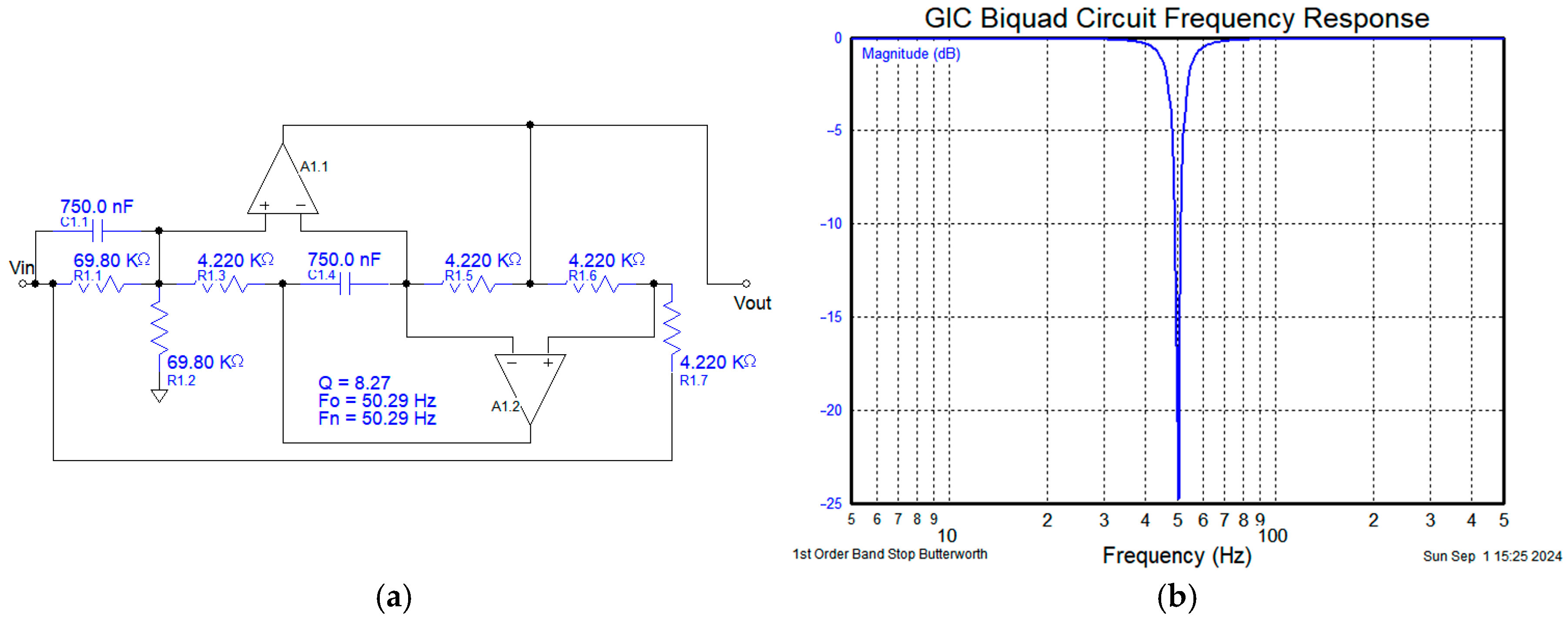
3.2. Notch and Band-Pass Filter Implementation

To mitigate the influence of the fundamental frequency component on subsequent filtering stages and to reduce the order of the filter, an active GIC (generalized impedance converter)-type filter is employed to implement a notch filter at 50 Hz. The dual-T filter circuit is illustrated in Figure 6.

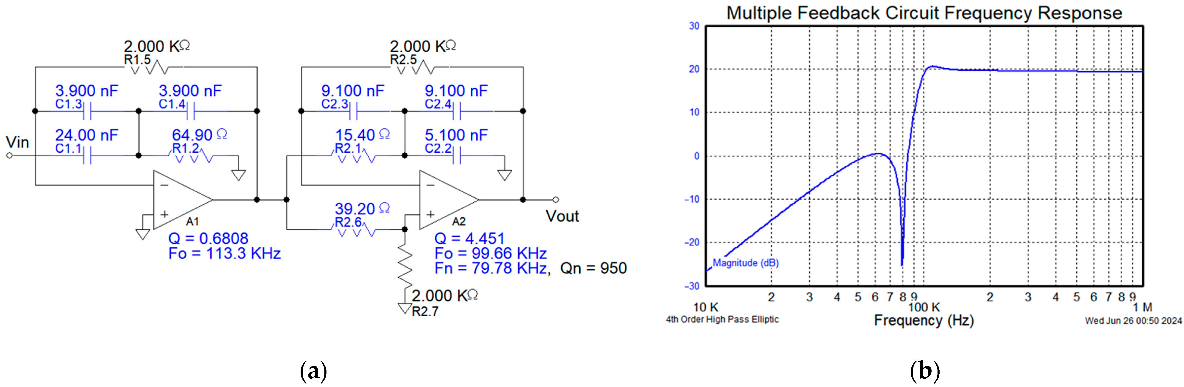
By balancing performance and cost, the high-pass filter is designed as a fourth-order elliptical high-pass filter with a cutoff frequency corresponding to a gain of 10. The filter is of the multiple feedback (MFB) type, as illustrated in Figure 7.

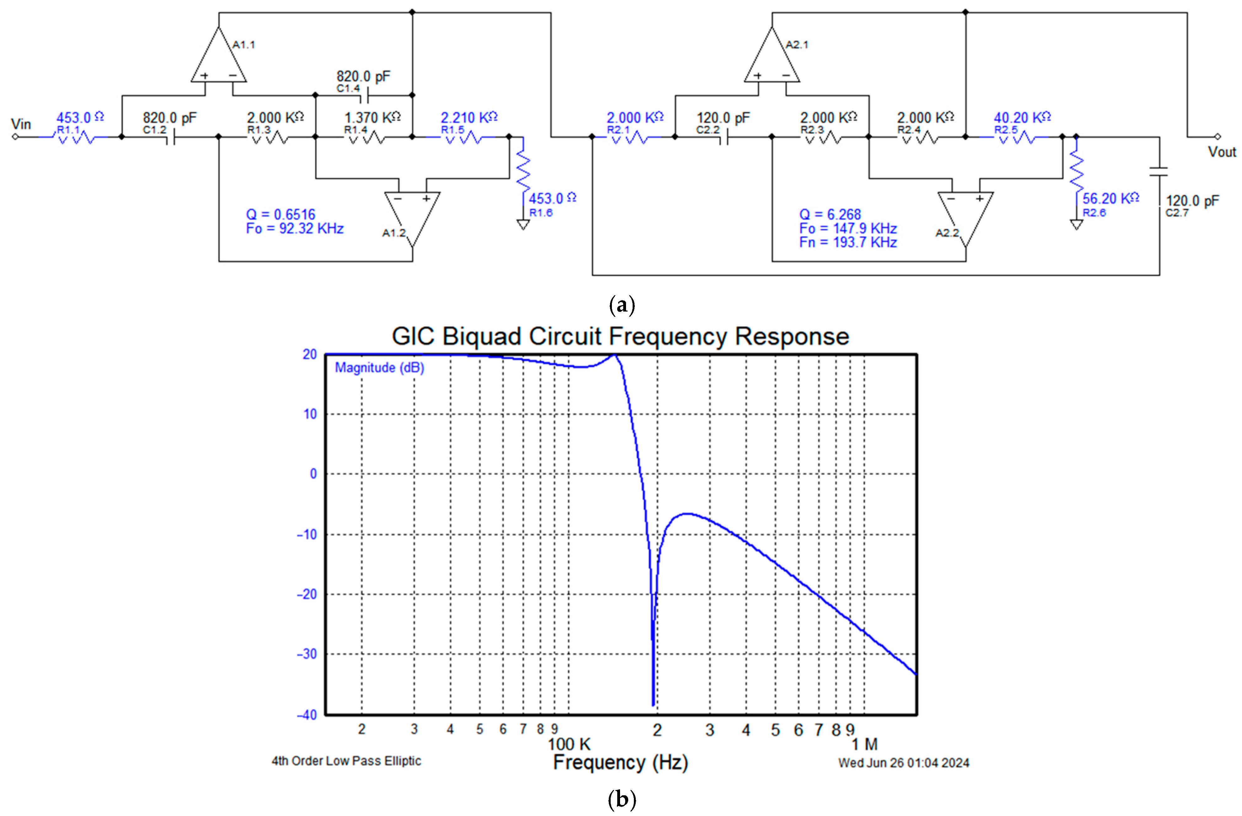
The low-pass filter is designed as a fourth-order elliptical filter, utilizing a GIC-type double second-order structure with a gain of 10. The filter structure and frequency response are illustrated in Figure 8.

3.3. High-Speed Comparator and ADC Acquisition

The high-speed comparator selected is the TLV3501, which features a rise time of 2 ns and operates in hysteresis comparator mode. The comparator threshold is adjusted using the DAC output integrated within the microcontroller (MCU). Due to the limitations of the band-pass filter, an anti-aliasing filter is not required for the ADC; instead, the AC signal is offset by 1.6 V to convert it into a DC signal. The ADC is configured for 12-bit resolution and a sampling rate of 1 MSPS, with direct memory access (DMA) triggering data transfer, thereby simplifying the circuit, which is omitted for brevity.

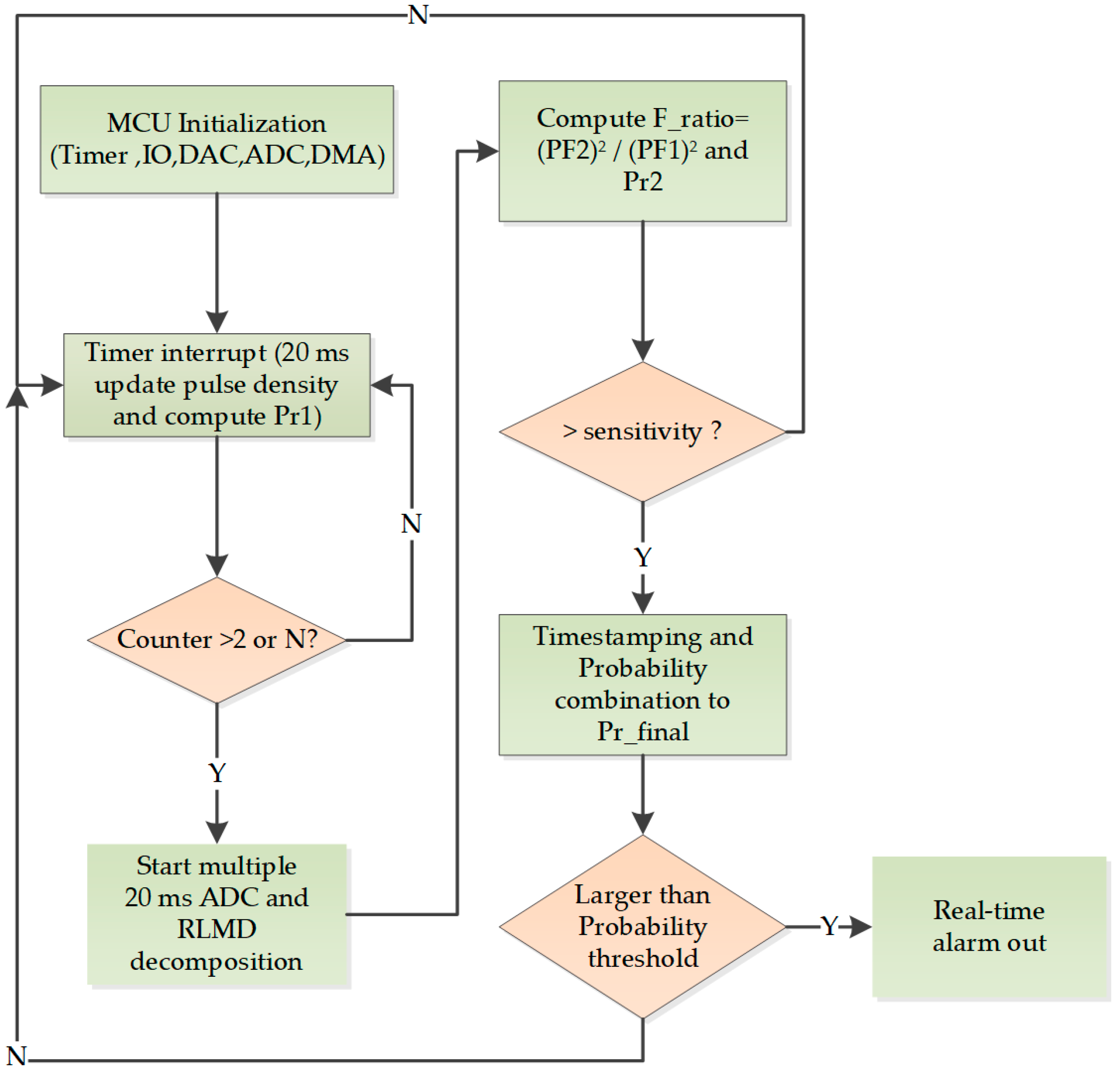
3.4. Software Flowchart

The occurrence of fault arcs repeats with a 20 ms power-frequency cycle. The system employs the low-cost STM32F series microcontroller, using a direct-drive C-language implementation to enhance efficiency and real-time performance. The overall software process is illustrated in Figure 9.

The system first initializes the hardware and peripherals, followed by configuring a high-speed timer to count the number of pulses on the IO pin at 20 ms intervals. This provides the pulse density value $a(t_0)$ for the current time, forming the first criterion. Due to the bandwidth limitations of the filter, the maximum value of $a(t_0)$ is $200\mathrm{k}/50=4\mathrm{k}$, with a maximum of 4k pulses per cycle.

Next, a comparison is made to check if $a(t_0)$ exceeds a predefined threshold $a_0$ (defaulted at 2 but can be adjusted to decrease sensitivity). If this threshold is exceeded, ADC sampling, DMA transfer, and the algorithm analysis unit are triggered. The RLMD decomposition and component strength ratio are computed efficiently, forming the second criterion. $F_{ratio}$ is then compared to a base threshold, and if exceeded, the detection probabilities from both branches are combined. The fault arc probability ${\mathrm{Pr}}_{final}$ is calculated. If this value exceeds a preset probability threshold, an alarm is triggered (i.e., setting the IO pin to a high level, with the rising edge used to trigger the AFCI). Real-time requirements are met if the output delay is less than 1 ms.

4. Experimental Platform and Analysis Verification

4.1. Fault Arc Detector and Testing Platform

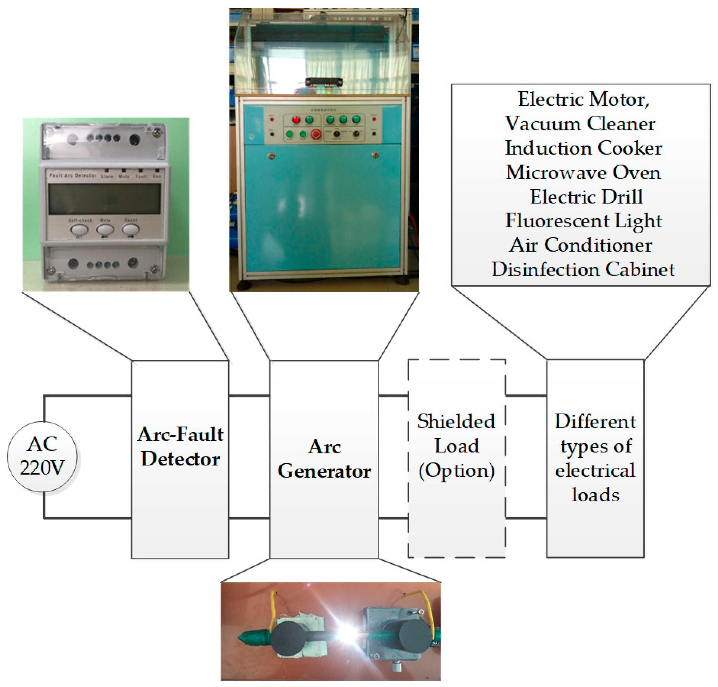
In accordance with the requirements of the Chinese national standard GB 14287.4, an experimental platform was constructed, as shown in Figure 10. The arc generator employs a micrometer-adjustable sliding stage to control the gap between a carbon rod and a copper rod with conical tips, achieving a positioning accuracy of 0.01 mm. This setup enables the simulation of arc generation under various resistive and inductive loads. In addition, the parallel arc test structure was modified to a simple parallel configuration.

4.2. Time–Frequency Data Analysis

Current data from fault arc events under various load types were obtained through data acquisition and subjected to time–frequency analysis. The fault arc waveforms and corresponding time–frequency representations for several typical loads are shown in Figure 11. These include current waveforms under both normal operation and fault arc conditions for an electric kettle.

The time–frequency analysis reveals that, during fault arc occurrences, the high-frequency components experience a 20–30 dB increase in intensity, and the spectrum exhibits quasi-continuous characteristics. This provides the analytical foundation for RLMD decomposition and arc fault detection.

4.3. Construction of the Experimental Platform

Figure 12 presents waveform diagrams of fault arcs occurring in both inductive and resistive loads. In the plots, voltage is shown in green, current in yellow, and the shaped pulse signal in purple. It can be observed that the current waveform exhibits increased high-frequency spikes during fault arcs, and that the pulse density after high-frequency band-pass filtering increases significantly during these spike events. In Figure 13a, the resistive load current shows clear interruptions near the zero-crossing points, with millisecond-scale zero-current intervals. In contrast, Figure 13b shows no obvious current interruption in the inductive load. Therefore, the presence of arc faults cannot be determined solely based on the discontinuity of the current waveform.

During testing with different loads, high-frequency pulses always occur when an arc fault is generated, with the pulse density varying significantly. In one cycle, the minimum number of pulses is one, while the maximum can reach several hundred (theoretically up to 4000 pulses, as the arc does not burn consistently throughout a cycle and includes idle periods). For high-sensitivity pulse count thresholds (with a pulse count of 2), the detection probability is 100%, and the false alarm probability is between 5% and 8%. For medium-sensitivity pulse count thresholds (with a pulse count of 5), the detection probability is 96%, and the false alarm probability is between 0.8% and 1%. For low-sensitivity pulse count thresholds (with a pulse count of 10), the detection probability is 92%, with a false alarm probability of around 0.5%. The occurrence of an arc always leads to an increase in pulse density, making pulse density one of the key criteria for fault arc detection. To further improve the detection probability and reduce the false alarm rate, RLMD component criteria are also introduced.

4.4. RLMD Data Analysis

The fault arc currents of the electric iron and vacuum cleaner were collected, and the corresponding PF waveform components were obtained through RLMD algorithm decomposition, as shown in Figure 13.

The RLMD decomposition algorithm exhibits temporal locality, which enables precise localization of waveform features in the time domain. By applying RLMD to the current waveform, the resulting PF components show a descending order in characteristic frequency, with PF₁ representing the highest frequency component. A feature ratio component $F_{ratio}$ is constructed from the PFs to estimate the probability of fault arc occurrence, denoted as $Pr2$.

Experimental results show that during periodic fault arc events, the value of $Pr2$ varies within the range of 0.1 to 0.95, effectively enabling the intermittent localization of arc occurrence cycles. For example, in the case of a resistive load (electric iron) experiencing arc faults, when $Pr1=0.85$ and $Pr2=0.7$, the combined detection probability is ${\mathrm{Pr}}_{final}=0.955$. In the case of an inductive load (vacuum cleaner), with $Pr1=0.72$ and $Pr2=0.88$, the final probability reaches ${\mathrm{Pr}}_{final}=0.9664$.

At the level of algorithmic engineering, a comparative analysis was conducted between the RLMD and pulse density algorithms proposed in this paper and the methods in references [25,26], as shown in

Table 1. Comparative analysis of different algorithms.

Algorithm	Algorithm Complexity	Sampling Frequency	Hardware Implementation	Hardware Optimization	Real-Time
Pulse density + RLMD	Low	12.8 kHz	Yes	Yes	Yes
Wavelet transform [25]	Middle	1 MHz	Yes	Yes	Yes
Convolutional neural network [26]	High	1 MHz	Yes	No	Yes

. The algorithm proposed in this article has certain advantages in algorithm complexity, signal sampling frequency, etc., and is particularly suitable for low-cost and low-power application fields.

5. Conclusions

To meet the demands of practical engineering applications, this study proposes a fault arc detection method based on the joint decision-making of pulse density and RLMD decomposition. The approach features strong hardware–software generality, flexible parameter tuning, and excellent real-time performance. After analog preprocessing of the high-frequency signal components, pulse density is extracted, enabling arc event localization within 5 ms, thus eliminating the need for high-speed sampling. For low-frequency components, an adaptive RLMD decomposition algorithm is employed, which offers low computational complexity and effective fault localization. By integrating decision metrics from both pulse density and RLMD-derived features, the method achieves high detection probability, low false alarm rate, low cost, and high real-time performance, meeting comprehensive practical requirements.

Future research directions involve using a server to periodically collect fault arc waveforms and data from various loads, thereby continuously updating the RLMD template library and refining parameter thresholds. This will enable remote firmware updates (including algorithms and feature libraries), transforming the system into an intelligent fault arc detector.