Gross Domestic Product Forecasting Using Deep Learning Models with a Phase-Adaptive Attention Mechanism

Abstract

Forecasting GDP is a highly practical task in macroeconomics, especially in the context of rapidly changing economic environments caused by both economic and non-economic factors. This study proposes a deep learning model that integrates Long Short-Term Memory (LSTM) networks with a phase-adaptive attention mechanism (PAA-LSTM model) to improve forecasting accuracy. The attention mechanism is flexibly adjusted according to different phases of the economic cycle—recession, recovery, expansion, and stagnation—allowing the model to better capture temporal dynamics compared to traditional static attention approaches. The model is evaluated using GDP data from six countries representing three groups of economies: developed, emerging, and developing. The experimental results show that the proposed model achieves superior accuracy in countries with strong cyclical structures and high volatility. In more stable economies, such as the United States and Canada, PAA-LSTM remains competitive; however, its margin over simpler models is narrower, suggesting that the benefits of added complexity may vary depending on economic structure. These findings underscore the value of incorporating economic cycle phase information into deep learning models for macroeconomic forecasting and suggest a promising direction for selecting flexible forecasting architectures tailored to different country groups.

1. Introduction

Gross Domestic Product (GDP) is not only a fundamental indicator of a country’s economic size and health, but it also plays a central role in the design and adjustment of socio-economic development policies. Institutions such as the International Monetary Fund (IMF), the World Bank, and the Organisation for Economic Co-operation and Development (OECD) rely heavily on GDP forecasts to formulate decisions on interest rates, fiscal planning, infrastructure investment, and social programs. As highlighted in recent reports from OECD (2023) and IMF (2023), accurate GDP forecasting remains a crucial requirement for effective macroeconomic policy formulation, particularly in times of global uncertainty [1,2].

Timely and reliable GDP growth forecasts help minimize macroeconomic risks, support resource allocation decisions, and assist the private sector in planning investment strategies. However, the emergence of complex global challenges, such as pandemics, geopolitical instability, supply chain disruptions, and financial volatility, has increased the difficulty of forecasting economic performance using traditional linear methods.

Conventional time series models, including Autoregressive Integrated Moving Average (ARIMA) and Vector Autoregression (VAR), have long been applied in macroeconomic analysis. Nevertheless, these models assume linear and time-invariant relationships and often struggle to capture structural changes and nonlinear dependencies in economic data, particularly during periods of sudden shifts or regime transitions [3,4]. As a result, machine learning and deep learning models have gained traction in recent years for their ability to model complex temporal patterns.

Among deep learning models, Long Short-Term Memory (LSTM) networks have proven especially effective in macroeconomic forecasting tasks, due to their ability to retain long-term dependencies in sequential data. When combined with attention mechanisms, LSTM models can learn to focus selectively on key historical time steps, further improving their predictive capacity [5].

The attention mechanism, initially developed for natural language processing tasks by Bahdanau et al. (2014) [6], has since been adapted to economic time series modeling. For instance, Qin et al. (2017) [5] demonstrated that dual-stage attention significantly enhances LSTM performance in financial forecasting tasks. Despite these advances, most attention-based forecasting models remain limited in their adaptability: they apply the same attention strategy across all economic contexts, failing to account for cyclical shifts such as recessions, recoveries, expansions, or stagnations.

This lack of phase awareness poses a significant limitation. Economic theory, dating back to the classical business cycle work of Burns and Mitchell [7], emphasizes that macroeconomic indicators—including GDP, inflation, and unemployment—exhibit distinct patterns across different phases of the economic cycle. Models that treat all time steps uniformly may therefore miss important structural signals, reducing their accuracy and robustness.

To address this gap, this study proposes a novel deep learning model that integrates a Phase-Adaptive Attention Mechanism into a multi-layer LSTM architecture. The proposed PAA-LSTM model enables attention weights to adjust dynamically based on the current phase of the economic cycle—namely, recession, recovery, expansion, or stagnation. This design allows the model to capture phase-specific temporal dependencies and improve forecasting performance across diverse macroeconomic environments.

Our model is tested on GDP data from six countries representing developed, emerging, and developing economies. By evaluating the model’s performance across different economic structures and volatility levels, we aim to assess not only its accuracy but also its generalizability. The key contribution of this study lies in bridging the gap between deep learning and economic cycle theory by embedding phase-awareness directly into the model’s attention mechanism, enabling more adaptive, interpretable, and context-sensitive forecasts.

2. Related Work

Forecasting GDP growth is a crucial topic that has been explored from various perspectives in both economics and data science. Traditional models such as linear regression, autoregressive integrated moving average (ARIMA), vector autoregression (VAR), and nonlinear models like Markov Switching have long played important roles in economic time series analysis [8].

The ARIMA model, known for its structure based on the lagged values of the dependent variable and noise components, has been successfully applied in numerous empirical studies. Mourougane and Roma (2003) [9] demonstrated that incorporating economic sentiment indicators into the ARIMA model improved short-term GDP forecasting in euro area countries, although the model exhibited some instability during crisis periods. T. Abeysinghe [10] employed an ARIMA framework to forecast Singapore’s quarterly GDP using international trade data and showed that the model achieved reasonably accurate short-term predictions. Similarly, A. Meyler et al. [11] used ARIMA to forecast the Consumer Price Index (CPI) in Ireland, thereby indirectly inferring real GDP trends. This approach highlights the interrelationship between inflation and output in macroeconomic forecasting. Notably, the distinction between core and trend components of inflation—emphasized by Stock and Watson (2016) [12]—can significantly impact forecast accuracy when CPI is used as a proxy for economic performance. M. R. Abonazel and A. I. Abd-Elftah (2019) [13] applied ARIMA for long-term GDP forecasting in Egypt and found that the ARIMA(1, 1, 0) specification provided the best forecast based on AIC and MAPE criteria. In Bangladesh, Voumik and Smrity (2020) [14] utilized ARIMA to forecast per capita GDP, affirming its applicability in emerging economies. In the developing region context, Ghazo (2021) [15] applied ARIMA to forecast both GDP and CPI for Jordan, showing that the model remains effective even when working with limited data. In addition to classical ARIMA models, Seasonal ARIMA (SARIMA) has been widely recognized as an effective method for time series with seasonal structures, particularly in economic and financial forecasting. SARIMA extends ARIMA by incorporating seasonal autoregressive and moving average components, allowing it to model recurring patterns over fixed intervals such as months or quarters. For example, Hyndman and Athanasopoulos (2018) [16] provided a comprehensive overview of SARIMA’s effectiveness in capturing both long-term trends and seasonal fluctuations in macroeconomic data. While our study focuses on annual GDP growth data, which does not exhibit explicit seasonality, we recognize that SARIMA is a valuable approach for higher-frequency datasets, such as those measured quarterly or monthly.

Meanwhile, the VAR model—introduced by Sims (1980) [17] to address the issue of endogeneity among macroeconomic variables—has been widely used in GDP analysis and forecasting. Robertson et al. [18] developed a six-variable VAR model, including GDP, CPI, money supply, and interest rates, to forecast U.S. GDP growth. Their results showed that the use of light Bayesian priors significantly enhanced out-of-sample forecast accuracy. Similarly, Salisu et al. (2021) [19] implemented a global VAR model to forecast GDP growth across developing economies, illustrating the model’s flexibility in handling cross-country macroeconomic data.

Although linear econometric models such as ARIMA and VAR are valued for their interpretability and theoretical consistency, they also present several limitations. These models typically assume linear and time-invariant relationships and may underperform during periods of major economic shocks or when confronted with nonlinear or unstructured data. As a result, a growing body of recent research has turned to machine learning approaches—or hybrid models—to overcome these constraints [20].

To overcome the limitations of traditional linear models, machine learning and deep learning methods have been increasingly applied over the past decade. Among them, the Long Short-Term Memory (LSTM) network, a variant of the Recurrent Neural Network (RNN) proposed by Hochreiter and Schmidhuber (1997) [21], has demonstrated its ability to retain long-term dependencies and model complex nonlinear relationships in time series data. B. Oancea et al. (2024) [22] applied LSTM to forecast Romania’s quarterly GDP from 1995 to 2023 and found that it outperformed conventional econometric models in both accuracy and modeling flexibility. Furthermore, hybrid architectures such as the Convolutional Neural Network combined with Long Short-Term Memory (CNN-LSTM) and Bidirectional Long Short-Term Memory (Bi-LSTM) have also been explored to capture spatio-temporal features and bidirectional contextual information in time series data [23,24,25].

Building on the development of LSTM, a significant advancement in deep learning was the introduction of the attention mechanism, which revolutionized how time series are processed. Attention enables the model to assign dynamic weights to input time steps, allowing it to focus more effectively on critical information during forecasting. Bahdanau et al. (2014) [6] and Qin et al. (2017) [5] were among the first to apply attention mechanisms in economic time series forecasting, demonstrating that LSTM combined with attention outperformed standard LSTM models in financial prediction tasks.

An extension of the attention mechanism is the Transformer model, proposed by Vaswani et al. (2017) [26], which marked a major breakthrough in natural language processing, has since been adapted to other domains, including economic forecasting. With its ability to learn representations without relying strictly on sequential ordering, the Transformer offers potential advantages over both LSTM and traditional attention structures [27]. In economics, Li et al. (2025) [28] applied the Transformer to forecast stock prices and reported promising results. FX-spot forecasting using Transformer models has demonstrated the importance of time embeddings and sequence modeling complexity [29]. However, the Transformer model typically requires large datasets and significant computational resources, which limits its applicability to macroeconomic problems where data are often limited and discontinuous.

In response to the limitations of static attention and the data demands of Transformers, recent studies have focused on developing adaptive attention mechanisms. These mechanisms allow models to adjust attention weights dynamically based on specific data contexts or sequence lengths, instead of using fixed parameters across all inputs. Nevertheless, most current research has yet to incorporate economic cycle phases into attention structures, despite their foundational role in macroeconomic time series. Qiu, Wang, and Zhou (2020) [30] introduced an approach that combines Long Short-Term Memory (LSTM) networks with an attention mechanism to enhance time series forecasting, effectively capturing important temporal patterns. However, their method did not specifically adapt the attention mechanism based on different economic phases, instead applying it uniformly across the entire sequence. Hybrid models such as LSTM combined with Hidden Markov Models have been explored to capture regime-switching behavior in GDP forecasting [31]. According to the classical theory by Burns and Mitchell [7,32,33], indicators such as GDP, unemployment, and inflation typically follow cyclical patterns characterized by phases of recession, recovery, expansion, and stagnation. Neglecting these cyclical dynamics can substantially hinder a model’s ability to adapt in real time.

From this review, it is evident that significant progress has been made in applying deep learning to GDP forecasting. However, a critical gap remains in optimizing attention mechanisms to reflect different phases of the economic cycle. Enabling the model to adjust focus weights based on each phase, such as recession or expansion, could be key to improving both forecasting accuracy and stability. This gap serves as the main motivation for our study: to propose a Long Short-Term Memory model integrated with a phase-adaptive attention mechanism, which accounts not only for temporal dependencies but also for the underlying cyclical structure of economic data. This model holds promise for enhancing GDP forecasting performance in volatile environments and contributes a novel approach to combining deep learning and cyclical macroeconomic theory in modern forecasting systems.

3. Proposed Method

Based on the theoretical gaps identified in the related work, this paper proposes a novel deep learning model called PAA-LSTM (Phase-Aware Adaptive LSTM). This model integrates a multi-layer LSTM network with an attention mechanism designed to adapt to different phases of the economic cycle. Rather than learning purely from sequential time patterns, the model leverages phase information (recession, recovery, expansion, and stagnation) to improve its focus on key time steps within macroeconomic data. The overall architecture and operational mechanism are presented in the following sections.

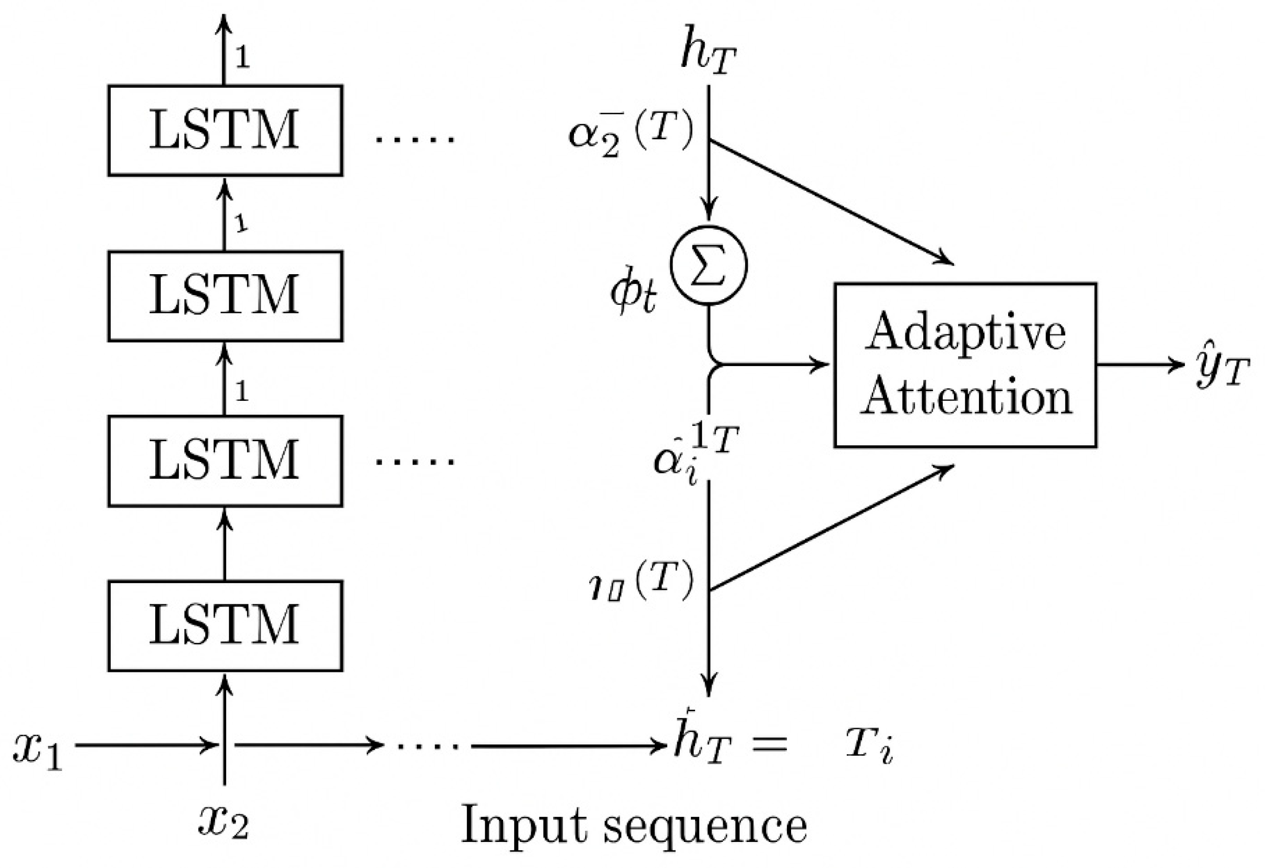
3.1. Model Architecture

The overall architecture of the PAA-LSTM model is composed of three main components: a multi-layer Long Short-Term Memory (LSTM) network, a Phase-Aware Adaptive Attention mechanism, and a fully connected output layer—Figure 1. The objective of this architecture is to leverage LSTM’s ability to model long-term dependencies and nonlinear relationships in time series data, while enhancing temporal flexibility and selective focus through a phase-adaptive attention mechanism.

-

Multi-layer LSTM: This component is responsible for extracting deep temporal features from the input time series, such as GDP growth, investment ratios, household consumption, and employment indicators. The use of multiple LSTM layers allows the model to learn abstract representations of macroeconomic dynamics;

-

Phase-Aware Adaptive Attention: Unlike standard attention mechanisms, this component is customized to adapt to each phase of the economic cycle (recession, recovery, expansion, and stagnation). Each phase is associated with a distinct set of attention parameters, enabling the model to prioritize critical time steps depending on the economic context;

-

Fully-connected output layer: This layer combines the contextual information from the LSTM and the attention mechanism to generate the final GDP growth forecast for the next time step.

The integration of these three components results in an architecture capable of capturing both long-term dependencies and dynamic cyclical patterns in macroeconomic data, making the model more adaptable and accurate in volatile economic environments.

In the proposed model, attention is no longer applied uniformly across the entire time series as in traditional models. Instead, it is designed to adapt dynamically to each phase of the economic cycle. This is achieved by mapping each phase (recession, recovery, expansion, slowdown) to a distinct set of attention weights. These weights adjust the model’s focus on specific time steps depending on the characteristics of each economic phase.

For example, during a recession, the model may assign higher weights to time steps associated with consumption and labor indicators. In contrast, during recovery or expansion phases, the model learns to adjust attention to focus more on investment or industrial production indicators.

As a result, the phase-adaptive attention mechanism enables the model to be more flexible while retaining the selective focus capability of standard attention but in a way that is better aligned with the dynamic nature of macroeconomic systems.

3.2. Phase-Adaptive Attention Representation in Economic Cycles

In the proposed model, the attention mechanism is designed to adapt to each phase of the economic cycle, rather than being applied statically as in traditional architectures. This process involves two key steps:

(1)

Segmenting the economic cycle into phases;

(2)

Mapping phase-specific attention weights accordingly.

3.2.1. Economic Phase Segmentation

The economic cycle in this study is divided into four typical phases: recession, recovery, expansion, and stagnation. This segmentation is grounded in classical business cycle theory developed by Burns and Mitchell [7,32,33], who first formalized the cyclical nature of macroeconomic indicators such as GDP, employment, and inflation. These four phases are commonly referenced in modern macroeconomic forecasting and business cycle research [32].

In this study, phase labels are assigned based on quantifiable rules derived from the growth rates of GDP. Specifically, negative growth indicates recession; positive but low growth indicates stagnation; strong consistent growth suggests expansion; and a rebound after recession marks recovery. These rules are adapted to reflect country-specific characteristics and are used to train the phase-aware attention mechanism.

3.2.2. Phase-Specific Attention Design

Each economic phase is associated with its own set of attention parameters (weight matrix and bias). At time step t, if the data belong to phase p, the attention weight is computed as

αₜᵖ = softmax(wᵖ · tanh(hₜ))

where

• αₜᵖ: the attention weight at time t in phase p;
• wᵖ: the trainable attention weight vector for phase p;
• hₜ: the hidden output of the LSTM at time t.

These attention weights are then used to compute a weighted average over the entire sequence of hidden states from the LSTM, as follows:

cₜ = ∑ₜ αₜᵖ · hₜ

The resulting context vector cₜ is then combined with the current LSTM output and passed to a dense layer to produce the predicted GDP growth. The detailed procedure of computing phase-specific attention weights is illustrated in Algorithm 1.

Training the attention mechanism in a phase-adaptive manner allows the model to dynamically adjust its temporal focus in alignment with the evolving structure of the economy. This improves both the forecasting accuracy and the stability of the model compared to standard attention mechanisms that lack phase awareness.

Algorithm 1 Pseudocode

Input:   H = [h1, h2, …, hₜ] // Hidden states from LSTM   P = [p1, p2, …, pₜ] // Phase labels for each time step   Wᵖ, bᵖ for each phase p ∈ {Recession, Recovery, Expansion, Stagnation} Output:     Context vector cₜ 1: Initialize attention weights α = [] 2: for t = 1 to T do 3:  Identify phaseₜ ← P[t] 4:  Retrieve parameters: W ← Wᵖ[phaseₜ], b ← bᵖ[phaseₜ] 5:  Compute energy: eₜ ← tanh(W · hₜ + b) 6:  Compute attention score: αₜ ← softmax(eₜ) 7:  Append αₜ to α 8: end for 9: Compute context vector: cₜ = ∑ (αₜ · hₜ) 10: Return cₜ Illustrative Example Assume T = 3, and the LSTM outputs are scalar values, as follows: t = [1, 2, 3]; h = [0.5, 1.0, −0.2] Phase: Recession Let wrecession = 0.8, and brecession = 0.1 Energy calculation:    e1 = tanh(0.8 × 0.5 + 0.1) = tanh(0.5) = 0.462    e2 = tanh(0.8 × 1.0 + 0.1) = tanh(0.9) = 0.716    e3 = tanh(0.8 × (−0.2) + 0.1) = tanh(−0.06) = −0.06 Softmax attention weights:    α1 = ${\displaystyle \frac{e^{0.462}}{e^{0.462}+e^{0.716}+e^{-0.06}}}$ ≈ 0.30    α2 = ≈ 0.47    α3 = ≈ 0.23 Context vector:    Crecession ≈ 0.30 × 0.5 + 0.47 × 1.0 + 0.23 × (−0.2) ≈ 0.41 Phase: Expansion Let wexpansion = 0.2, and bexpansion = 0 Energy calculation:    e1 = tanh(0.2 × 0.5) = tanh(0.1) = 0.1    e2 = tanh(0.2 × 1.0) = tanh(0.2) = 0.197    e3 = tanh(0.2 × (−0.2)) = tanh(−0.04) = −0.04 Softmax attention weights:    α ≈ [0.31, 0.34, 0.35] Context vector:    cexpansion ≈ 0.31 × 0.5 + 0.34 × 1.0 + 0.35 × (−0.2) ≈ 0.42 Interpretation

In the recession phase, the weight vector w^recessin has a large positive value, causing the model to assign greater attention to time steps with higher hidden states (e.g., t = 2). In the expansion phase, the attention scores are more evenly distributed across time steps. This reflects the model’s stable attention during growth periods, where GDP dynamics are often more gradual and less abrupt.

3.3. Phase-Wise Training Strategy

To ensure that the model effectively learns the dynamic structure of each phase in the economic cycle, the training process is designed with specific phase-adaptive strategies as follows:

• Phase-Based Data Segmentation

The entire dataset is first segmented into phases using a labeling algorithm. Each subset of the data, corresponding to a specific phase (recession, recovery, expansion, slowdown), is then used in combination with phase information as an additional input to the model.

• Phase-Weighted Loss Function

In the composite loss function, each phase is assigned a unique weight to adjust the learning priority. Phases with higher volatility—such as recession or recovery—receive larger loss weights, prompting the model to focus more on reducing errors in unstable conditions.

• Phase-Specific Hyperparameter Optimization

Hyperparameters such as learning rate, batch size, number of epochs, and dropout rate are individually optimized for each phase using grid search. This helps the model avoid overfitting or underfitting in phases with distinct characteristics.

• Phase-Wise Fine-Tuning

After overall training, the model is further fine-tuned for each specific phase using phase-wise fine-tuning techniques. In this stage, only the attention and dense layer parameters are updated, while the LSTM layers are kept fixed to preserve the core deep learning structure.

• Conditional Cross-Validation

Instead of randomly or sequentially splitting the training and testing datasets, the validation process is designed to ensure that each phase is represented in both sets. This allows the model to generalize its forecasting ability while maintaining sensitivity to cyclical behavior.

A potential concern with phase-based training is the reduction in sample size when the dataset is divided according to economic phases. While it is true that each phase utilizes only a subset of the full time series, this does not inherently compromise model performance if the training strategy is carefully designed. To address this, two effective approaches can be employed. First, the model can be pre-trained on the complete time series and subsequently fine-tuned within each economic phase. This strategy leverages the full data context while enabling the model to specialize in phase-specific dynamics. Alternatively, instead of splitting the data, the entire dataset can be used with phase labels incorporated as an additional input feature. This allows the model to learn phase-aware representations without reducing the size of the training set, thereby preserving sufficient data coverage even for less frequent phases. Both approaches maintain generalization capacity while enhancing the model’s ability to capture the distinct characteristics of each economic phase. As a result, they contribute to more accurate and stable GDP forecasting by improving the model’s adaptability to structural shifts in macroeconomic environments.

3.4. Procedure

The sequence of steps in our study is as follows:

• Preprocess and normalize the entire dataset using z-score standardization;
• Segment the economic cycle into four phases: recession, recovery, expansion, and slowdown;
• Train the PAA-LSTM model using phase-wise fine-tuning strategies;
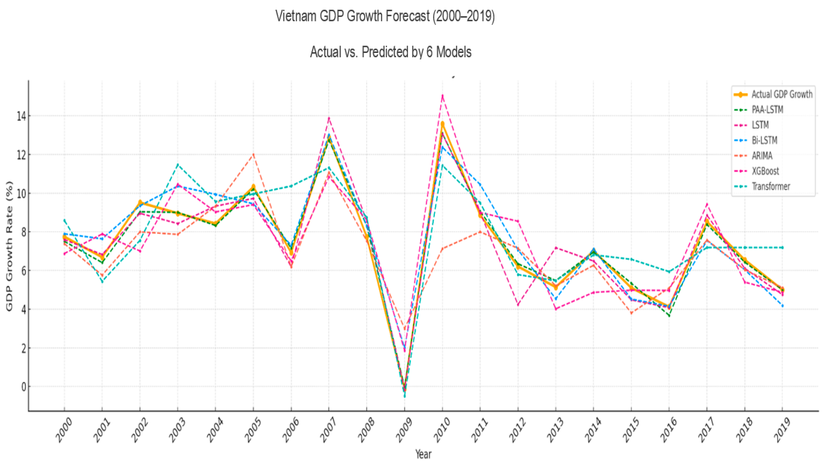
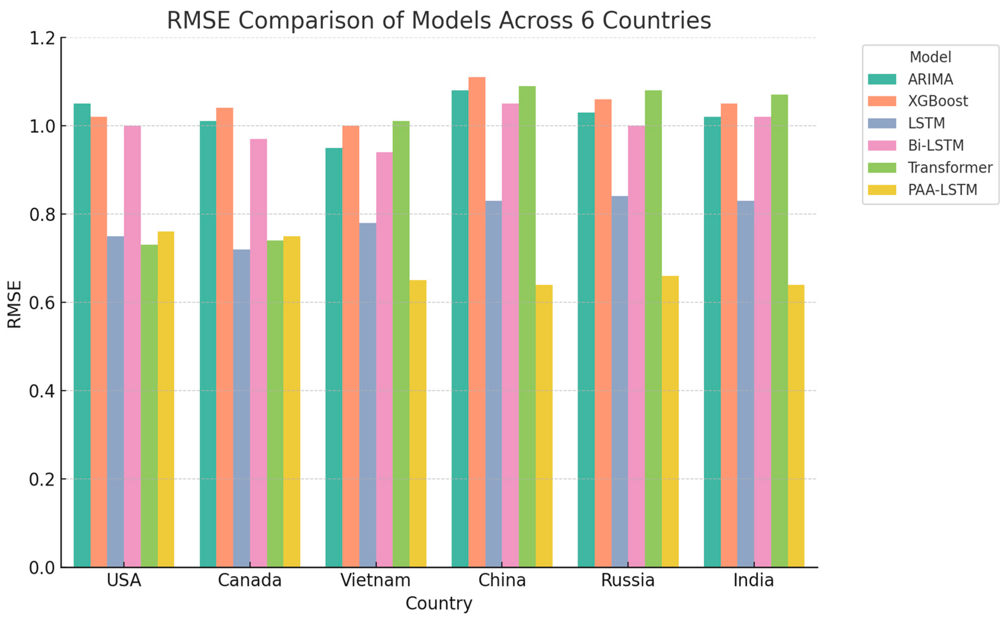
• Compare forecasting performance with baseline models: ARIMA, XGBoost, Transformer, LSTM, Bi-LSTM, and LSTM + Attention.

ARIMA: For each country, we applied the auto-ARIMA algorithm to automatically identify the optimal model configuration based on the Akaike Information Criterion (AIC). This ensured model parsimony while capturing temporal dependencies within the series.

XGBoost: The gradient boosting model was tuned using a grid search approach over key hyperparameters such as max_depth, learning_rate, and n_estimators, in combination with time-series cross-validation to prevent overfitting and ensure generalizability.

Transformer: The Transformer architecture consisted of two encoder layers, each with four attention heads. A fully connected output layer was added with dropout regularization. Hyperparameters were carefully calibrated to balance model complexity and forecasting performance, while avoiding overfitting in relatively small macroeconomic datasets.

LSTM, Bi-LSTM, and LSTM + Attention: These models were implemented using consistent input sequence lengths, hidden layer sizes, and optimization procedures. Regularization techniques such as dropout and early stopping were uniformly applied to ensure fair comparison across architectures.

• Evaluate the models

To evaluate the model’s performance, we use the Root Mean Squared Error (RMSE) as the primary metric for assessing prediction accuracy. RMSE measures the square root of the average of squared differences between predicted and actual values, providing a clear indication of how well the model fits the data. It is defined as

$$\mathrm{RMSE}=\sqrt{{\displaystyle \frac{1}{n}}{{\displaystyle \sum }}_{i=1}^n{\left(y_i-{\widehat{y}}_i\right)}^2}$$

where y_i is the actual value, ${\widehat{y}}_i$ is the predicted value, and n is the number of observations. A lower RMSE indicates better predictive performance.

4. Experiment and Discussion

4.1. Data and Scope

The study utilizes macroeconomic datasets from two main sources: the Penn World Table (PWT version 10.0) [34] and World Bank Open Data [35]. The dataset includes indicators such as real GDP growth (RGDP), household consumption, investment, government expenditure, price level components (PL variables), population, employed labor force, working hours, capital stock, exports, imports, and exchange rates. In addition, data on human capital are also integrated from the PWT.

The data are collected on an annual basis. The scope of application covers six countries representing three different economic groups:

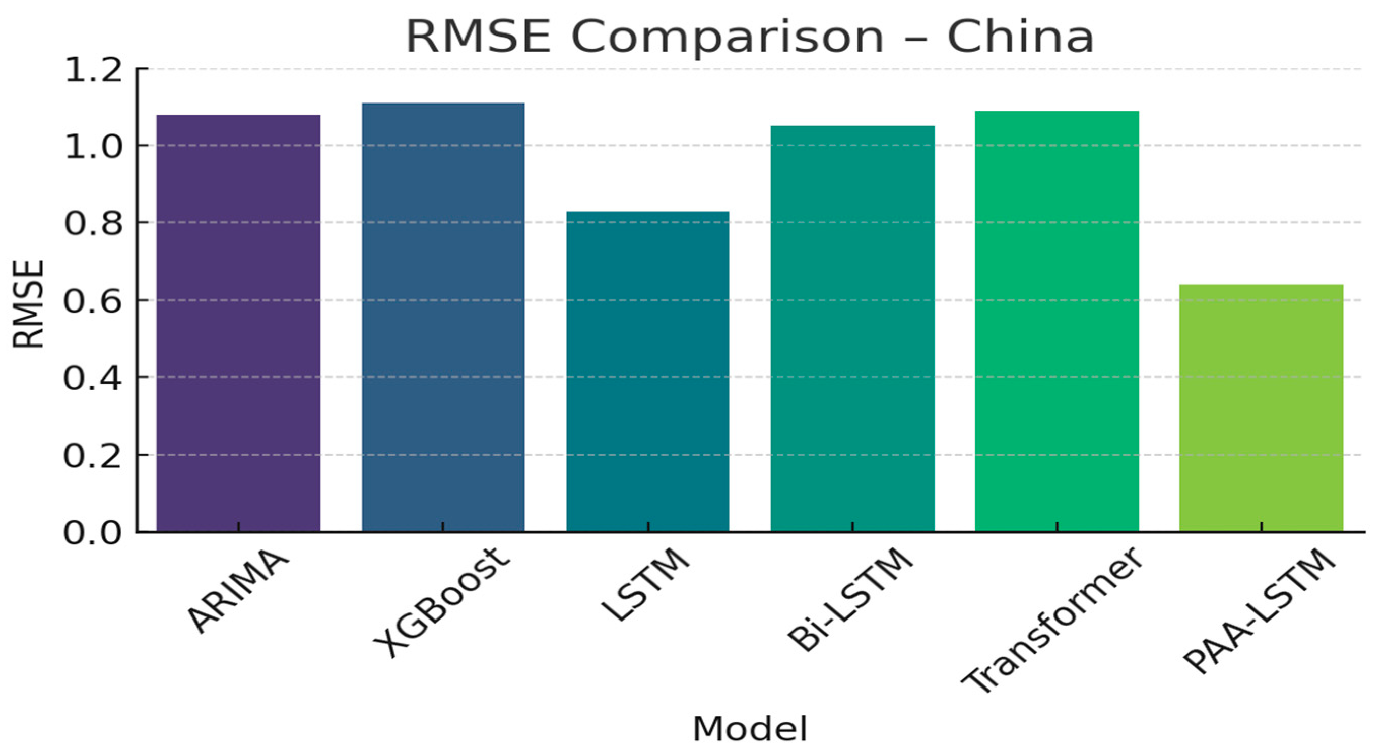
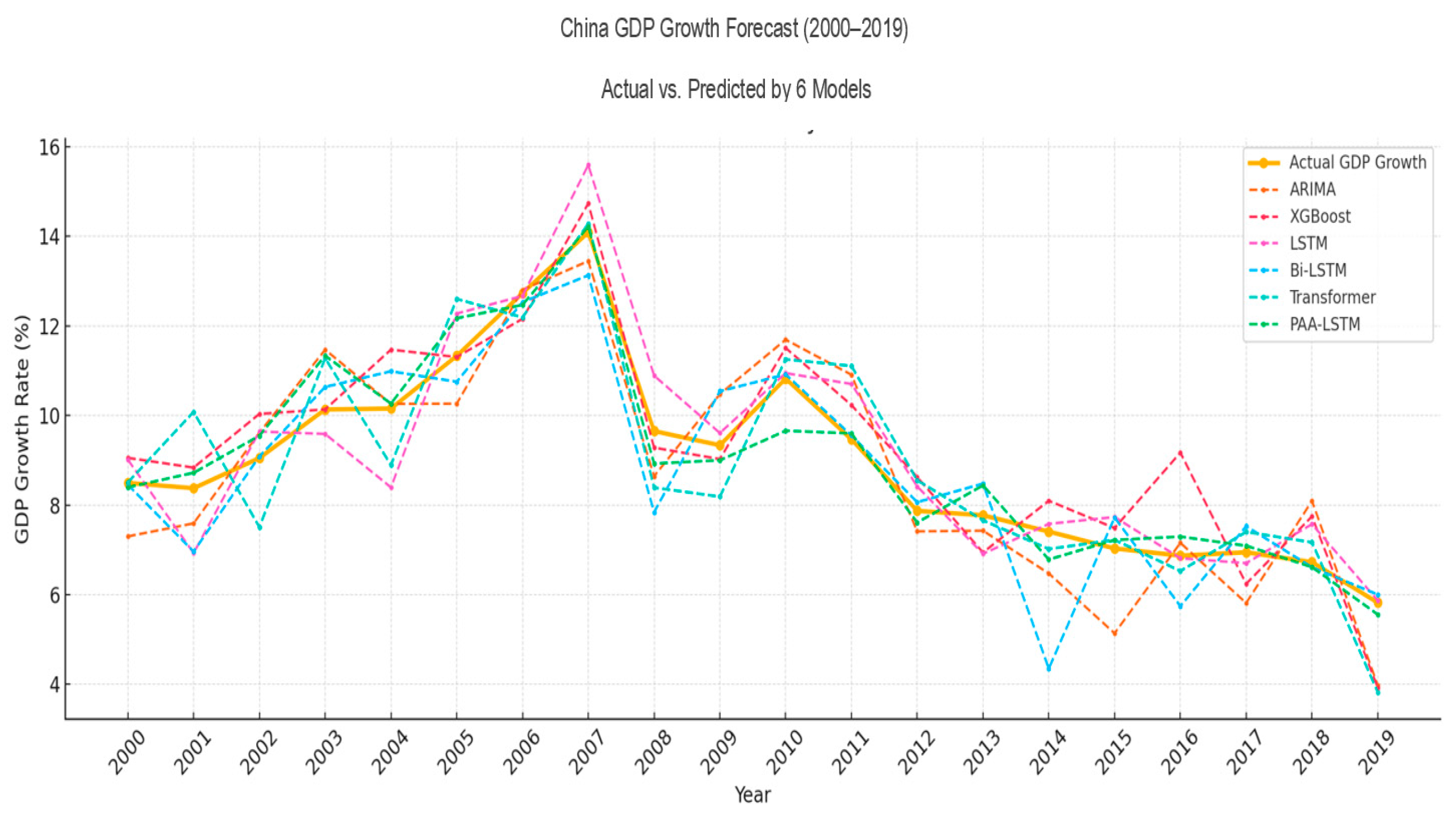
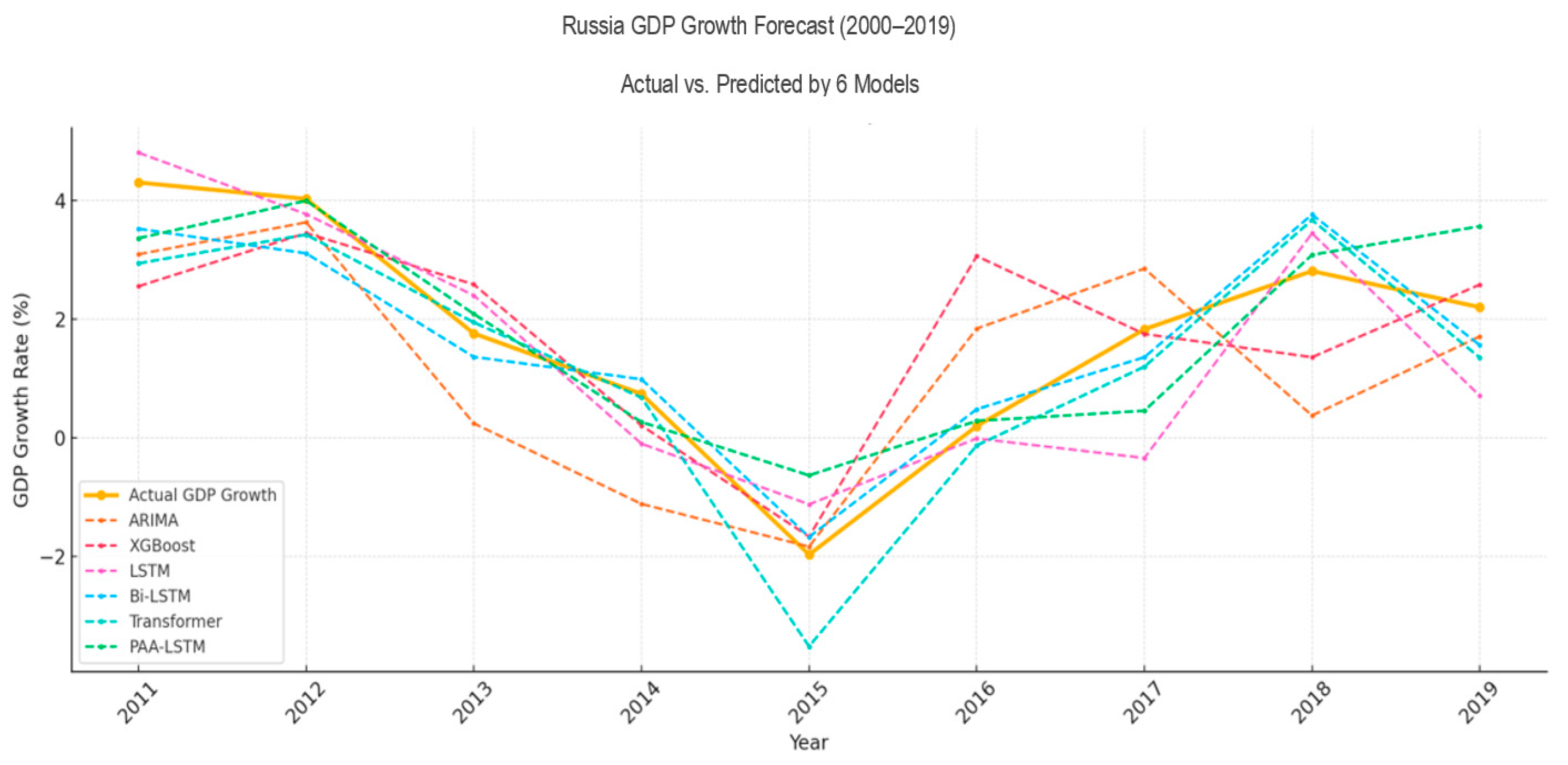
• Emerging economies: China, Russia;
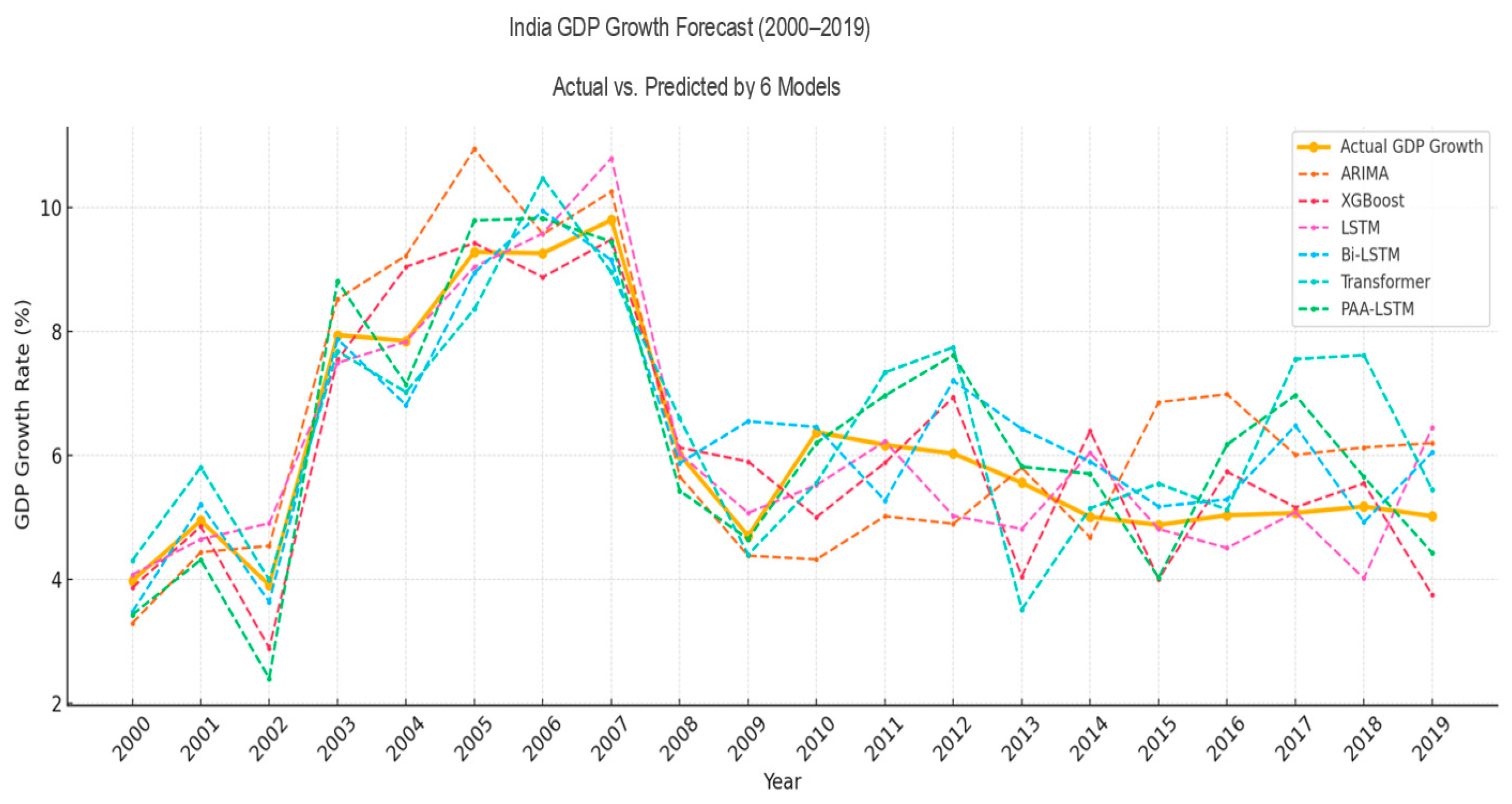
• Developing economies: Vietnam, India;
• Developed economies: United States, Canada.

The PWT database includes macroeconomic data for 183 countries from 1950 to 2019. We extracted data from 1980 to 2019 to maximize complete data coverage. For Russia, data are only available from 1991.

Data Preprocessing Steps

• Step 1: Remove missing, invalid, or inconsistent observations across data sources;
• Step 2: Construct additional economic interaction features, such as the product of human capital and employment rate (hc × emp), to enhance the model’s capacity to learn nonlinear patterns;
• Step 3: Structure the data as time series tables sorted by country and time, suitable for sequential deep learning training.

After collection, all indicators are standardized using z-score normalization to ensure consistency in units and scale across countries, which helps improve the learning efficiency of the deep learning models.

4.2. Experimental Results

All experiments were conducted on a dedicated workstation equipped with the following hardware: CPU: i9 9880H; Ram: 32G; SSD: 512G; and Card: Qudro T2000 4G.

The software environment used includes Python v3.10 with TensorFlow v2.13 and Keras (https://keras.io/). Additional libraries included Scikit-learn (v1.3), NumPy (v1.24), and Matplotlib (v3.7) [36].

Train/Test Split Strategy: For each country, the dataset was divided into training and testing sets using a chronological split. In each case, 80% of the earliest observations were used for training, and the remaining 20% were reserved for testing. This preserves the temporal structure of the data and avoids information leakage.

Cross-Validation Approach: In addition to the fixed train/test split, we employed an expanding window cross-validation strategy tailored for time series. The validation folds were constructed as follows:

• For countries with data from 1980 to 2019:

  ○

  Fold 1: Train = 1980–1999, Test = 2000–2004;

  ○

  Fold 2: Train = 1980–2004, Test = 2005–2009;

  ○

  Fold 3: Train = 1980–2009, Test = 2010–2014;

  ○

  Fold 4: Train = 1980–2014, Test = 2015–2019.

• For Russia (data from 1991 to 2019):

  ○

  Fold 1: Train = 1991–2010, Test = 2011–2014;

  ○

  Fold 2: Train = 1991–2014, Test = 2015–2019.

This time-aware cross-validation ensures that the model is evaluated across different economic conditions while preserving causality. Moreover, each validation fold includes different phases of the economic cycle (recession, recovery, expansion, and stagnation), allowing the phase-adaptive attention mechanism to be rigorously tested under realistic forecasting scenarios.

The experimental results are presented through performance evaluation tables of various models across six countries. The models compared include ARIMA, XGBoost, LSTM, Bi-LSTM, Transformer, and the proposed PAA-LSTM.

Below are the experimental results and illustrative charts, which highlight the differences in forecasting performance among the models across countries.

Table 1. Vietnam GDP forecast results.

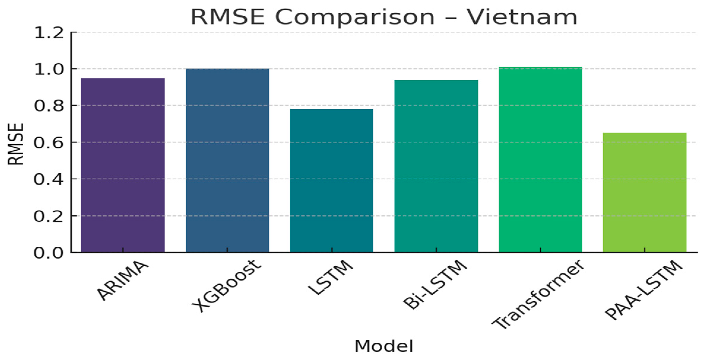
Model	RMSE	MAE	R2
ARIMA	0.95	0.73	0.76
XGBoost	1.0	0.97	0.84
LSTM	0.78	0.61	0.75
Bi-LSTM	0.94	1	0.79
Transformer	1.01	0.83	0.82
PAA-LSTM	0.65	0.48	0.94

and Figure 2 and Figure 3 present the detailed GDP forecasting results for Vietnam across different machine learning models. Among the models evaluated, PAA-LSTM achieves the best performance with RMSE = 0.65, MAE = 0.48, and R² = 0.94. This demonstrates the superior modeling capability of the proposed model in the context of volatile economic data.

Compared to traditional LSTM (RMSE = 0.78, R² = 0.75), PAA-LSTM significantly improves forecasting accuracy by leveraging the phase-adaptive attention mechanism, which enables the model to focus more effectively on key time periods. Furthermore, PAA-LSTM outperforms classical machine learning models such as ARIMA (RMSE = 0.95) and XGBoost (RMSE = 1.00), which lack the ability to learn complex nonlinear and long-term dependencies.

Although Transformer is also a powerful architecture (R² = 0.82), it still results in RMSE = 1.01 and MAE = 0.83 -s substantially higher than PAA-LSTM. This indicates that incorporating economic phase information into attention mechanisms enables deep learning models to better capture critical macroeconomic signals across different stages. The results in Vietnam clearly demonstrate the advantage of the phase-adaptive attention approach in the context of developing economies, where data tend to be unstable and are strongly influenced by cyclical factors.

After evaluating the model’s performance in Vietnam, we proceeded to assess its effectiveness in India—a developing country that also serves as a representative of emerging economies.

Table 2. India GDP forecast results.

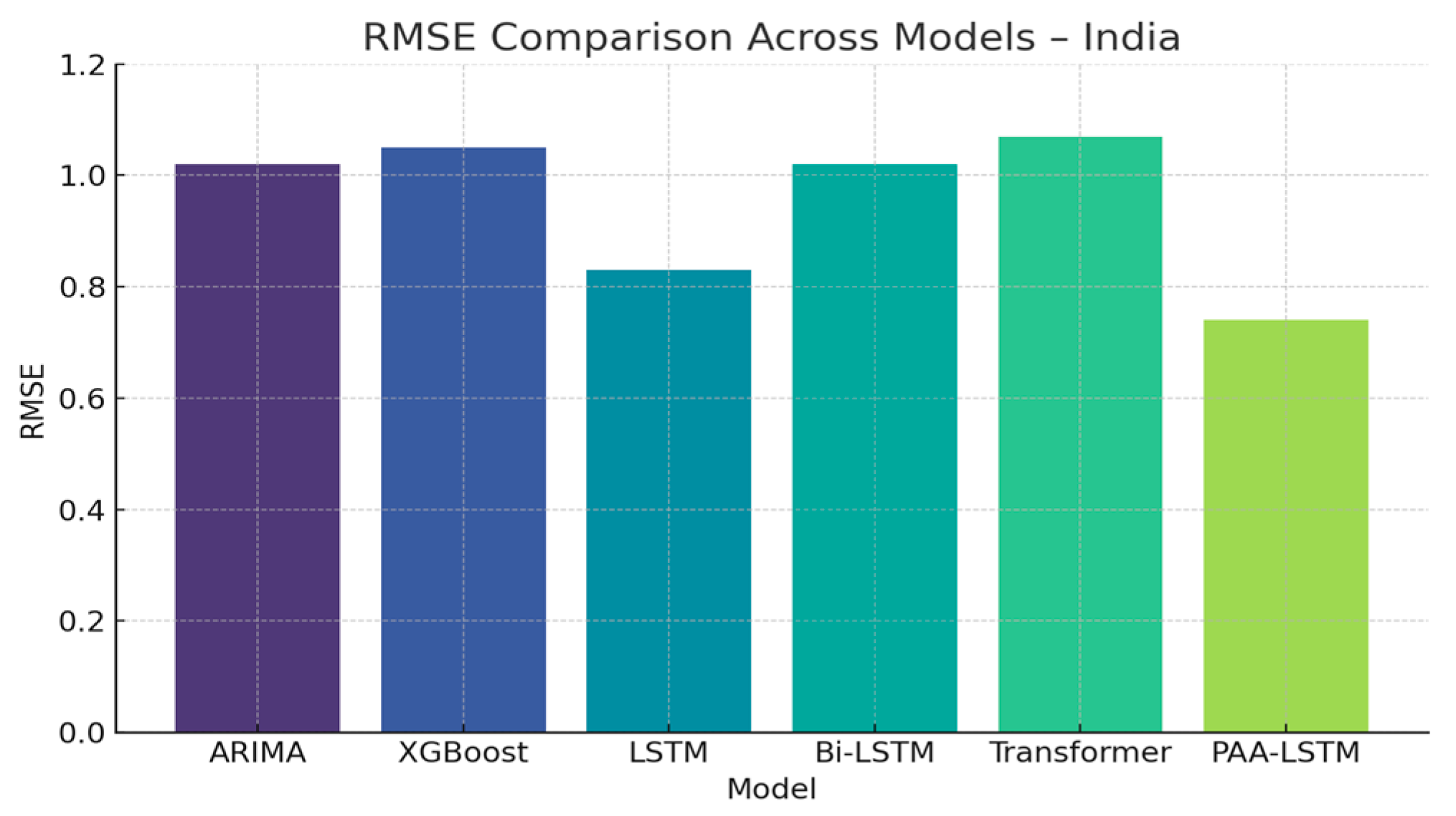
Model	RMSE	MAE	R2
ARIMA	1.02	0.78	0.83
XGBoost	1.05	0.95	0.87
LSTM	0.83	0.66	0.77
Bi-LSTM	1.02	0.86	0.84
Transformer	1.07	0.91	0.84
PAA-LSTM	0.74	0.48	0.95

, Figure 4 and Figure 5 detail the forecasting results in this context. PAA-LSTM continues to demonstrate superior performance, achieving RMSE = 0.74, MAE = 0.48, and R² = 0.95, outperforming all baseline models. Notably, compared to Bi-LSTM and Transformer, which have RMSE values of 1.02 and 1.07, respectively, the proposed model significantly reduces forecasting errors.

This highlights the critical role of phase-adaptive attention in enabling the model to learn economic behaviors that exhibit cyclical and time-varying characteristics. With its flexibility to adapt to structural changes, PAA-LSTM proves well-suited for dynamic economic environments like India, where investment, production, and consumption frequently fluctuate due to both policy shifts and market forces.

Next, the GDP forecasting results for China and Russia further support the effectiveness of the proposed PAA-LSTM model. In China,

Table 3. China GDP forecast results.

Model	RMSE	MAE	R2
ARIMA	1.08	0.9	0.78
XGBoost	1.11	0.71	0.85
LSTM	0.83	0.55	0.85
Bi-LSTM	1.05	0.78	0.8
Transformer	1.09	0.86	0.82
PAA-LSTM	0.64	0.5	0.8

and Figure 6 and Figure 7 PAA-LSTM achieved an RMSE of 0.64, significantly lower than other models such as Transformer (RMSE = 1.09), Bi-LSTM (1.05), and XGBoost (1.11). It also attained superior MAE and R² values, with MAE = 0.47 and R² = 0.96. These results indicate the model’s strong ability to capture the cyclical patterns of a fast-growing and complex economy like China.

With regard to Russia,

Table 4. Russia GDP forecast results.

Model	RMSE	MAE	R2
ARIMA	1.03	0.9	0.77
XGBoost	1.06	0.83	0.78
LSTM	0.84	0.61	0.78
Bi-LSTM	1.0	0.9	0.91
Transformer	1.08	0.96	0.83
PAA-LSTM	0.69	0.49	0.89

, Figure 8 and Figure 9 pertain to another emerging economy. The PAA-LSTM model achieved an RMSE of 0.81, which is lower than that of Transformer (1.08), Bi-LSTM (1.00), and ARIMA (1.03). With MAE = 0.66 and R² = 0.90, the model demonstrated not only lower average error but also strong explanatory power. These findings align with expectations that economies exposed to external shocks, such as energy price volatility and geopolitical tension, would benefit greatly from models capable of adapting to different economic phases.

Finally, the GDP forecasting results for the United States and Canada—two developed economies—reveal a different pattern. With regard to the United States,

Table 5. US GDP forecast results.

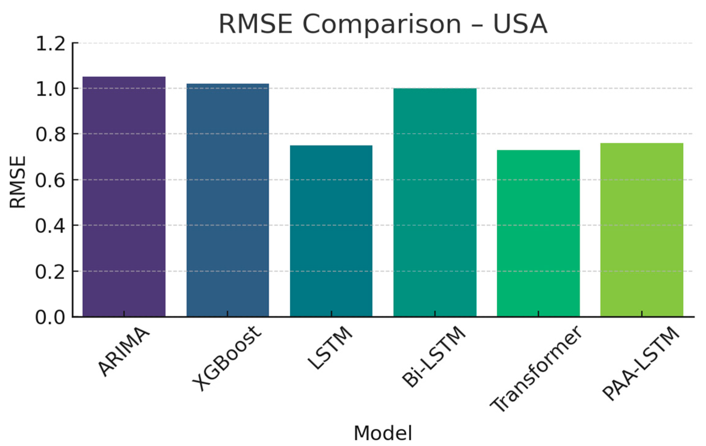
Model	RMSE	MAE	R2
ARIMA	1.05	0.8	0.79
XGBoost	1.02	0.79	0.87
LSTM	0.75	0.57	0.81
Bi-LSTM	1	0.9	0.86
Transformer	0.73	0.98	0.76
PAA-LSTM	0.76	0.47	0.89

, Figure 10 and Figure 11 pertain to the PAA-LSTM model, which achieved an RMSE of 0.76 and R² of 0.89, slightly behind Transformer (RMSE = 0.73) in terms of error but surpassing it in explanatory power. Meanwhile, traditional models like ARIMA (RMSE = 1.05) and XGBoost (RMSE = 1.02) showed significantly higher errors. This suggests that in stable data environments, basic LSTM or Transformer architectures can still perform well without the need for phase-adaptive attention.

In the case of Canada,

Table 6. Canada GDP forecast results.

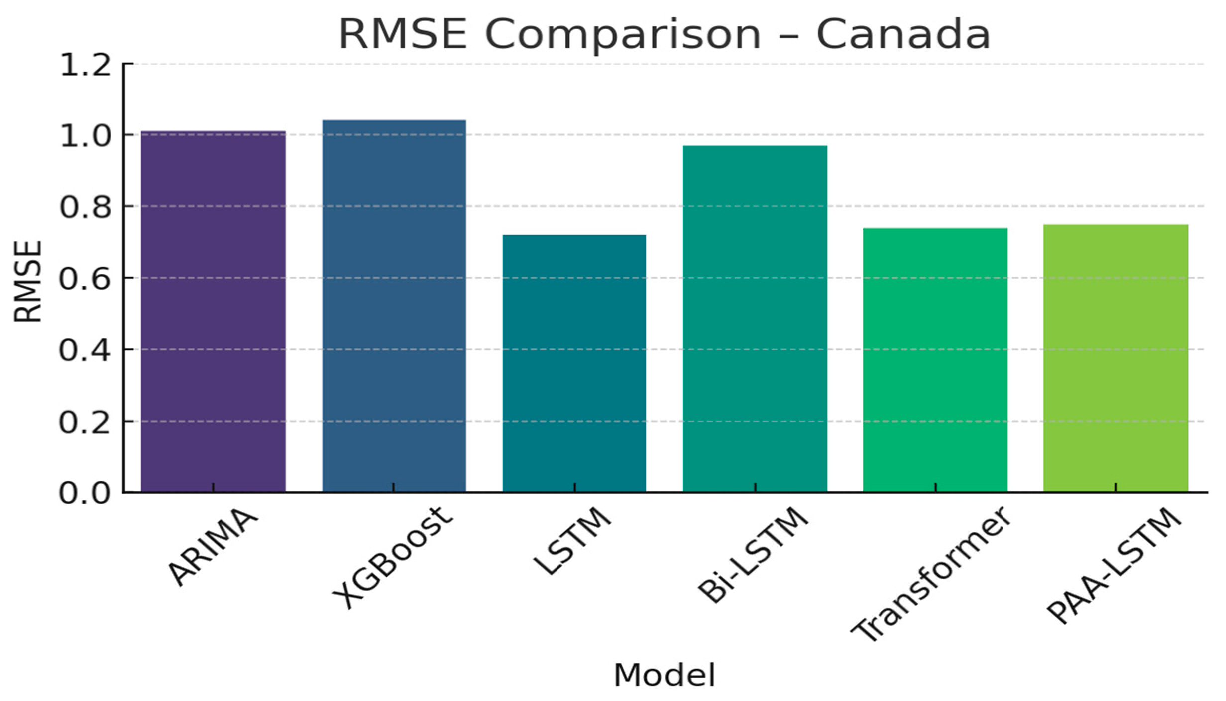
Model	RMSE	MAE	R2
ARIMA	1.01	0.73	0.76
XGBoost	1.04	0.79	0.82
LSTM	0.72	0.59	0.82
Bi-LSTM	0.97	0.83	0.77
Transformer	0.74	0.98	0.82
PAA-LSTM	0.75	0.48	0.9

, Figure 12 and Figure 13 pertain to the forecasting results that reveal a competitive landscape among the evaluated models. The LSTM model achieves the lowest RMSE value of 0.72, closely followed by Transformer (0.74) and PAA-LSTM (0.75). However, despite not having the lowest RMSE, PAA-LSTM demonstrates the strongest overall performance with the lowest MAE (0.48) and the highest R² value of 0.90.

These results indicate that while PAA-LSTM may not always outperform other models in terms of absolute error, it consistently provides better explanatory power and stability, an advantage especially relevant in macroeconomic settings where model interpretability is important. For developed countries, the PAA-LSTM model still achieves very promising results, particularly in terms of generalization and stability. Overall, the PAA-LSTM model exhibits strong and flexible GDP forecasting capabilities across various economic conditions, reinforcing the value of incorporating economic cycle dynamics into the attention mechanism for macroeconomic forecasting

4.3. Discussion

The experimental results across six countries—representing developed, emerging, and developing economies—as shown in Figure 14, demonstrate the strong performance and adaptability of the PAA-LSTM model. This section expands upon these results by comparing them with findings from prior studies, assessing how the current approach aligns with or diverges from existing research.

The PAA-LSTM model consistently achieves the lowest or near-lowest RMSE in volatile economies such as Vietnam, China, and India. This confirms earlier observations by Qiu et al. (2020) [30] and Qin et al. (2017) [5], who emphasized the value of attention mechanisms in capturing complex temporal dynamics. However, while these prior models used static attention, our results demonstrate that incorporating economic phase information further enhances forecasting accuracy, especially during transition periods like recessions or recoveries.

In contrast to traditional models like ARIMA and XGBoost, which assume linearity and time invariance, our model performs better across nearly all cases, aligning with findings by Oancea et al. (2024) [22], Chen et al. (2025) [37] and Jallow et al. (2025) [38], who reported that deep learning models outperform linear econometric techniques. Notably, in our experiments, ARIMA and XGBoost consistently rank among the least effective, with RMSE often exceeding 1.0.

In comparison with recent studies applying LSTM-based models, our results validate the advantage of phase-adaptive attention. For example, Xie et al. (2024) [39] showed that deep learning performance varies across countries depending on economic complexity and data stability. Our model expands upon that by dynamically adjusting to country-specific cyclical patterns, resulting in higher R² scores across diverse settings.

The Transformer model, despite its success in NLP and other domains (Vaswani et al., 2017) [26], shows inconsistent results in macroeconomic forecasting in our study. This aligns with Li et al. (2025) [28], who noted that Transformers require large datasets and may struggle with sparse or discontinuous economic data. It is important to emphasize that economic phases are inherently latent variable—they are not directly observable in real time and can only be approximated based on available indicators. This limitation has been well acknowledged in the regime-switching literature, such as the classical model by Hamilton (1989) [40], which treats economic regimes as unobservable and inferred through probabilistic structures. Following this theoretical foundation, our study adopts a practical approximation by defining economic phases using simple rule-based thresholds applied to real GDP growth rates. These empirical signals serve as effective proxies for latent cycle states and are derived directly from observable data, making them suitable for integration into deep learning workflows. Unlike traditional regime-switching models that require complex inference procedures, our approach enables efficient and transparent modeling of cyclical dynamics within the attention mechanism, thereby enhancing model interpretability and applicability in real-world forecasting tasks.

Interestingly, our findings suggest that Bi-LSTM does not yield a performance edge over standard LSTM in macroeconomic contexts. This echoes conclusions by Fan et al. (2024) [24], who indicated that the directional causality of macroeconomic indicators may limit the benefits of bidirectional architectures.

For stable economies such as the United States and Canada, PAA-LSTM still maintains competitive accuracy, but the margin over simpler models narrows. This supports observations by Kant et al. (2024) [41] and Vataja and Kuosmanen (2023) [42], who found that model complexity does not always translate to significant accuracy gains in low-variance environments. In such contexts, economic indicators tend to evolve more smoothly and with fewer abrupt structural shifts, reducing the advantage conferred by phase-adaptive mechanisms. Furthermore, in these cases, the benefit of capturing cyclical transitions is diminished, and the additional layers of complexity in the PAA-LSTM architecture may not yield proportional improvements in performance. Instead, standard LSTM or Transformer models, which are already proficient in modeling stable time series, can perform similarly or even slightly better in terms of RMSE.

Overall, our study extends the deep learning literature on GDP forecasting by demonstrating that phase-adaptive attention is particularly valuable in volatile macroeconomic environments. It also suggests that future research should consider adaptive model selection strategies—choosing models based on structural characteristics of the economy being forecasted.

5. Conclusions

This study proposed the PAA-LSTM model, which integrates multi-layer LSTM networks with a phase-adaptive attention mechanism to improve the accuracy of GDP growth forecasting. Unlike traditional attention mechanisms, PAA-LSTM enables the model to adjust its focus dynamically according to different phases of the economic cycle, such as recession, recovery, expansion, and stagnation. Experimental evaluations across six countries—representing developed, emerging, and developing economies—demonstrated the superior performance of PAA-LSTM. The model consistently achieved the lowest RMSE in most countries, particularly in volatile economic contexts like Vietnam, China, and India. In more stable economies like the United States and Canada, the model still performs competitively; however, the advantage over simpler models is reduced. This suggests that while phase-adaptive attention offers clear benefits in dynamic settings, its added complexity may yield diminishing returns in low-variance contexts. Compared to traditional models such as ARIMA and XGBoost and even advanced deep learning architectures like LSTM, Bi-LSTM, and Transformer, the proposed model exhibited stronger modeling capabilities by effectively capturing nonlinear relationships and long-term dependencies in macroeconomic time series. Notably, the integration of economic phase information into the attention mechanism has proven to be an effective strategy for adapting to structural shifts in economic data over time. Recent studies have suggested leveraging large-scale panel microdata as a promising approach to enhance GDP growth prediction [43]. Future research could explore directions such as incorporating alternative data sources (e.g., Google Trends [44], social media, satellite imagery) to enhance early detection of economic dynamics; applying Explainable AI (XAI) methods like SHAP and LIME to improve the transparency and interpretability of GDP forecasts [45]; and developing real-time phase detection modules to optimize the model’s adaptability to rapidly changing economic conditions. In addition, expanding the scope of experimental validation to include a larger and more diverse set of countries and regions, encompassing various stages of economic development and geographical contexts, would help enhance the model’s robustness and generalizability. This broader evaluation could provide deeper insights into the PAA-LSTM model’s applicability across different macroeconomic systems [46,47]. Overall, the PAA-LSTM model opens a promising new pathway toward enhancing the accuracy and robustness of modern macroeconomic forecasting systems.

References

- OECD. OECD Economic Outlook; OECD Publishing: Paris, France, 2023; Volume 2023, Issue 2; Available online: https://www.oecd.org/en/publications/oecd-economic-outlook/volume-2023/issue-2_7a5f73ce-en.html (accessed on 15 January 2025).
- IMF. World Economic Outlook, October 2023: Navigating Global Divergences; International Monetary Fund: Washington, DC, USA, 2023; Available online: https://www.imf.org/en/Publications/WEO/Issues/2023/10/10/world-economic-outlook-october-2023 (accessed on 15 January 2025).
- Păun, E.; Dima, M. The relevance of ARIMA models in financial forecasting under volatility and structural uncertainty. Theor. Appl. Econ. 2022, XXIX, 5–22. Available online: https://store.ectap.ro/articole/1222.pdf (accessed on 20 January 2024).
- MASEconomics. Structural Breaks in Time Series Analysis: Managing Sudden Changes. 2023. Available online: https://maseconomics.com/structural-breaks-in-time-series-analysis-managing-sudden-changes/ (accessed on 10 January 2025).
- Qin, Y.; Song, D.; Cheng, H.; Cheng, W.; Jiang, G.; Cottrell, G. A dual-stage attention-based recurrent neural network for time series prediction. In Proceedings of the Twenty-Sixth International Joint Conference on Artificial Intelligence, Melbourne, Australia, 19–25 August 2017; pp. 2627–2633. [Google Scholar] [CrossRef]
- Bahdanau, D.; Cho, K.; Bengio, Y. Neural machine translation by jointly learning to align and translate. arXiv 2014, arXiv:1409.0473. [Google Scholar]
- Burns, A.; Mitchell, W. Measuring Business Cycles; National Bureau of Economic Research: Cambridge, MA, USA, 1946. [Google Scholar]
- Hamilton, J.D. Time Series Analysis; Princeton University Press: Princeton, NJ, USA, 1994. [Google Scholar]
- Mourougane, A.; Roma, M. Can confidence indicators be useful to predict short-term real GDP growth? Appl. Econ. Lett. 2003, 10, 519–522. [Google Scholar] [CrossRef]
- Abeysinghe, T. Forecasting Singapore’s quarterly GDP with monthly external trade. Int. J. Forecast. 1998, 14, 505–513. [Google Scholar] [CrossRef]
- Meyler, A.; Kenny, G.; Quinn, T. Forecasting Irish Inflation Using ARIMA Models. Central Bank of Ireland, Technical Paper 3/RT/98. 1998. Available online: https://www.centralbank.ie/docs/default-source/publications/research-technical-papers/3rt98---forecasting-irish-inflation-using-arima-models-(kenny-meyler-and-quinn).pdf (accessed on 15 December 2024).
- Stock, J.H.; Watson, M.W. Core Inflation and Trend Inflation. Rev. Econ. Stat. 2016, 98, 770–784. [Google Scholar] [CrossRef]
- Abonazel, M.R.; Abd-Elftah, A.I. Forecasting egyptian gdp using arima models. Rep. Econ. Financ. 2019, 5, 35–47. Available online: https://www.m-hikari.com/ref/ref2019/ref1-2019/p/abonazelREF1-2019.pdf (accessed on 20 January 2024). [CrossRef]
- Voumik, L.C.; Smrity, D.Y. Forecasting GDP per capita in Bangladesh: Using ARIMA model. Eur. J. Bus. Manag. Res. 2020, 5, 1–5. [Google Scholar] [CrossRef]
- Ghazo, A. Applying the ARIMA Model to the Process of Forecasting GDP and CPI in the Jordanian Economy. Int. J. Financ. Res. 2021, 12, 70–85. [Google Scholar] [CrossRef]
- Hyndman, R.J.; Athanasopoulos, G. Forecasting: Principles and Practice, 2nd ed.; Monash University: Melbourne, Australia, 2018; Available online: https://otexts.com/fpp2/ (accessed on 20 January 2024).
- Sims, C.A. Macroeconomics and reality. Econom. J. Econom. Soc. 1980, 48, 1–48. [Google Scholar] [CrossRef]
- Robertson, J.C.; Tallman, E.W. Vector autoregressions: Forecasting and reality. Econ. Rev. Fed. Reserve Bank Atlanta 1999, 84, 4. [Google Scholar]
- Salisu, A.A.; Gupta, R.; Olaniran, A. The effect of oil uncertainty shock on real gdp of 33 countries: A global var approach. Appl. Econ. Lett. 2021, 30, 269–274. [Google Scholar] [CrossRef]
- Maccarrone, G.; Morelli, G.; Spadaccini, S. GDP Forecasting: Machine Learning, Linear or Autoregression? Front. Artif. Intell. 2021, 4, 757864. [Google Scholar] [CrossRef]
- Hochreiter, S.; Schmidhuber, J. Long short-term memory. Neural Comput. 1997, 9, 1735–1780. [Google Scholar] [CrossRef] [PubMed]
- Oancea, B. Advancing GDP Forecasting: The Potential of Machine Learning Techniques in Economic Predictions. arXiv 2025, arXiv:2502.19807. [Google Scholar] [CrossRef]
- Staffini, A. A CNN–BiLSTM Architecture for Macroeconomic Time Series Forecasting. Eng. Proc. 2023, 39, 33. [Google Scholar] [CrossRef]
- Fan, Y.; Tang, Q.; Guo, Y.; Wei, Y. BiLSTM-MLAM: A Multiscale Time Series Forecasting Model Based on BiLSTM and Local Attention Mechanism. Sensors 2024, 24, 3962. [Google Scholar] [CrossRef] [PubMed]
- Widiputra, H.; Mailangkay, A.; Gautama, E. Multivariate CNN-LSTM Model for Multiple Parallel Financial Time-Series Prediction. Complexity 2021, 2021, 9903518. [Google Scholar] [CrossRef]
- Vaswani, A.; Shazeer, N.; Parmar, N.; Uszkoreit, J.; Jones, L.; Gomez, A.; Kaiser, Ł.; Polosukhin, I. Attention is all you need. arXiv 2017, arXiv:1706.03762. [Google Scholar] [CrossRef]
- Xu, C.; Li, J.; Feng, B.; Lu, B. A Financial Time-Series Prediction Model Based on Multiplex Attention and Linear Transformer Structure. Appl. Sci. 2023, 13, 5175. [Google Scholar] [CrossRef]
- Li, S.; Schulwolf, Z.B.; Miikkulainen, R. Transformer based time-series forecasting for stock. arXiv 2025, arXiv:2502.09625. [Google Scholar]
- Fischer, T.; Sterling, M.; Lessmann, S. Fx-spot predictions with state-of-the-art transformer and time embeddings. Expert Syst. Appl. 2024, 249, 123538. [Google Scholar] [CrossRef]
- Qiu, J.; Wang, B.; Zhou, C. Forecasting stock prices with long-short term memory neural network based on attention mechanism. PLoS ONE 2020, 15, e0227222. [Google Scholar] [CrossRef]
- Zhang, J.; Wen, J.; Yang, Z. China’s GDP forecasting using Long Short Term Memory Recurrent Neural Network and Hidden Markov Model. PLOS ONE 2022, 17, 1–17. [Google Scholar] [CrossRef]
- Zarnowitz, V. Business Cycles: Theory, History, Indicators, and Forecasting; University of Chicago Press: Chicago, IL, USA, 1992. [Google Scholar]
- Blanchard, O.; Johnson, D.R. Macroeconomics, 7th ed.; Pearson: Boston, MA, USA, 2017. [Google Scholar]
- Feenstra, R.; Inklaar, R.; Timmer, M. The next generation of the Penn World Table. Am. Econ. Rev. 2015, 105, 3150–3182. Available online: https://www.rug.nl/ggdc/productivity/pwt/ (accessed on 15 January 2024). [CrossRef]
- World Bank. World Development Indicators. Available online: https://data.worldbank.org (accessed on 15 January 2025).
- Hull, I. Machine Learning for Economics and Finance in TensorFlow 2: Deep Learning Models for Research and Industry; Apress: Berkeley, CA, USA, 2021. [Google Scholar]
- Chen, X.-S.; Kim, M.G.; Lin, C.; Na, H.J. Development of Per Capita GDP Forecasting Model Using Deep Learning: Incorporating CPI and Unemployment. Sustainability 2025, 17, 843. [Google Scholar] [CrossRef]
- Jallow, H.; Mwangi, R.W.; Gibba, A.; Imboga, H. Transfer Learning for Predicting GDP Growth Based on Remittance Inflows: A Case Study of The Gambia. Front. Artif. Intell. 2025, 8, 1510341. [Google Scholar] [CrossRef]
- Xie, H.; Xu, X.; Yan, F.; Qian, X.; Yang, Y. Deep Learning for Multi-Country GDP Prediction: A Study of Model Performance and Data Impact. arXiv 2024, arXiv:2409.02551. Available online: https://arxiv.org/abs/2409.02551 (accessed on 15 January 2025).
- Hamilton, J.D. A new approach to the economic analysis of nonstationary time series and the business cycle. Econometrica 1989, 57, 357–384. [Google Scholar] [CrossRef]
- Kant, D.; Pick, A.; de Winter, J. Nowcasting GDP using machine learning methods. AStA Adv. Stat. Anal. 2024, 109, 1–24. Available online: https://link.springer.com/article/10.1007/s10182-024-00515-0 (accessed on 16 January 2025).
- Vataja, J.; Kuosmanen, P. Forecasting GDP Growth in Small Open Economies: Foreign Economic Activity vs. Domestic Financial Predictors. SSRN Electron. J. 2023. Available online: https://papers.ssrn.com/sol3/papers.cfm?abstract_id=4415388 (accessed on 25 January 2024).
- Cui, Y.; Hong, Y.; Huang, N.; Wang, Y. Forecasting GDP Growth Rates: A Large Panel Micro Data Approach. SSRN Electron. J. Feb. 2025. Available online: https://papers.ssrn.com/sol3/papers.cfm?abstract_id=5151633 (accessed on 5 May 2025).
- Choi, H.; Varian, H. Predicting the present with Google Trends. Econ. Rec. 2012, 88, 2–9. [Google Scholar] [CrossRef]
- Liu, D.; Chen, K.; Cai, Y.; Tang, Z. Interpretable EU ETS Phase 4 Prices Forecasting Based on Deep Generative Data Augmentation. Financ. Res. Lett. 2024, 61, 105038. [Google Scholar] [CrossRef]
- Gatti, R.; Lederman, D.; Islam, A.M.; Nguyen, H.; Lotfi, R.; Mousa, M.E. Data Transparency and GDP Growth Forecast Errors. J. Int. Money Financ. 2024, 140, 102991. Available online: https://openknowledge.worldbank.org/entities/publication/0fd1d195-9a75-430f-80ca-070332af36c6 (accessed on 15 January 2025). [CrossRef]
- Lesmy, D.; Muchnik, L.; Mugerman, Y. Lost in the fog: Growing complexity in financial reporting—A comparative study. Res. Sq. 2024; preprint. [Google Scholar] [CrossRef]