Optimal Configuration of Feeder Terminal Units in Power Distribution Networks Considering Distributed Generation

Abstract

This paper proposes an optimization strategy for Feeder Terminal Unit (FTU) configuration in distribution networks, accounting for the influence of Distributed Generation (DG). Firstly, the impact of different FTU configurations on load interruption duration was analyzed. Regions were divided based on the planned installation locations of FTUs, and a model for calculating load interruption losses in different regions was established. Secondly, an all-probability model was introduced to calculate the probability of DG disconnection during faults. The importance weight of DG was determined based on its capacity, and a loss model for photovoltaic disconnection was constructed accordingly. Then, an optimization configuration model was established with the objective of minimizing the weighted sum of FTU installation costs, load interruption losses, and DG disconnection losses, while constraining the solution by supply reliability. Finally, the accuracy of the proposed optimization model was validated using Particle Swarm Optimization (PSO) through the IEEE 33-node distribution network model.

1. Introduction

The vast majority of power outages are caused by short-circuit faults in distribution networks. To ensure continuous operation of the distribution system during fault conditions, it is imperative to rapidly locate the faulty section and isolate the affected line segment, thereby maintaining power supply to unaffected portions of the network. From the perspective of fault location objectives, the methodologies can be primarily categorized into two types: fault section localization and fault distance measurement [1,2]. The fault distance measurement method is primarily employed in traditional distribution networks characterized by extended power supply distances and challenging line inspection conditions [3,4]. The primary function of this methodology is to assist maintenance personnel in rapidly and accurately pinpointing fault locations, thereby significantly reducing outage duration while enhancing grid reliability and operational safety. Fault distance measurement typically relies on electrical parameters during fault conditions (e.g., voltage/current waveforms) to estimate the fault location. Various methodologies have been developed for fault distance calculation, each with distinct technical characteristics: impedance-based methods [5], traveling-wave-based fault location methods [6], and model-based fault location methods [7]. Fault section localization refers to the process of identifying the specific line segment or segment range where a fault occurs. It is primarily employed for rapid fault screening in distribution networks, enabling utilities to quickly isolate the affected section while maintaining service in healthy portions of the grid. Feeder automation (FA), as an important component of the distribution automation system, can achieve rapid fault location, isolation, and restoration [8,9,10,11], thereby improving the reliability of power supply. The Feeder Terminal Unit (FTU) is responsible for transmitting the collected data to the master station, and the master station conducts fault location and issues processing instructions [12]. According to functions, FTUs can be divided into “two-telemetry” terminals and “three-telemetry” terminals. The “two-telemetry” terminals have the functions of remote measurement and remote signaling, while the “three-telemetry” terminals include remote measurement, remote signaling, and remote-control functions. The types and quantities of FTUs directly affect the efficiency of fault location and isolation in the distribution network [13]. At the same time, when there is no FTU configured between the Distributed Generation (DG) and the fault point, the fault isolation process will cause the DG to be disconnected from the grid, unable to support the reliable power supply of the non-fault area, thus resulting in resource waste and off-grid loss costs.

Therefore, how to reasonably arrange the installation locations and types of FTUs, achieve a balance between power supply reliability and economy, and give full play to the supporting role of DG in power supply restoration is the problem to be solved in this paper. In reference [14], the method of “centralized collection, zonal application” is adopted to divide the distribution area into six categories. According to the collected information of the power supply area, the configuration strategies of full two-telemetry and full three-telemetry terminals are used to estimate the number of FTUs. Reference [15] approximately determines the optimal configuration quantity of FTUs from the perspectives of input/output and power supply reliability. Reference [16] divided the power supply area into six categories according to the requirements of power supply reliability and proposed using differential design principles for the configuration of FTUs, communication, and relay protection based on the regional categories. These studies start at the overall distribution network, analyze the overall power outage time of the lines, and provide approximate solutions for the quantity and location of FTUs. Reference [17] obtained the power outage time function of the load under different equipment configurations by defining logical operators. Reference [18] proposed a calculation method for the power outage time of users under different anticipated fault conditions and constructed an equipment optimization configuration model with the goal of minimizing the sum of switch investment costs, operation and maintenance costs, and user power outage loss costs. Reference [19] used the mixed-integer programming method to construct an equipment configuration model, aiming to minimize the total configuration cost and the cost of load terminals. Although the above methods, respectively, consider the power outage time of the fault area and the non-fault area, most of the studies treat the power outage time of the fault area as a fixed value, and do not fully consider the influence of the types of FTUs upstream and downstream of the fault area on the power outage time.

Some studies have considered the output model of DG, and on this basis, have established a mathematical analysis model of the distribution network that takes into account the grid-connected operation of DG. For example, reference [20] studied the optimal configuration problem of FTUs under the access of DG. With the objective function of minimizing the number of FTUs, relevant constraints were established and an analysis model was constructed on the premise of ensuring the observability of the distribution network. Reference [21] established a probability model of the output power of DG, and comprehensively considered the investment cost, operation and maintenance cost, and power outage loss to construct an optimization model for the selection of distribution terminals. However, these methods fail to fully consider the losses caused by the disconnection of DG within the fault area due to fault isolation after the occurrence of a fault [22].

In summary, there are two key gaps in existing research: first, the dynamic impact of FTU types (two-telemetry and three-telemetry) on power outage time in fault areas has not been deeply quantified; second, the loss costs of DG after faults have been ignored. This paper aims to fill the above research gaps by establishing an FTU type location optimization model, fully considering the differentiated effectiveness of FTU types in upstream and downstream fault areas and incorporating DG loss costs into the optimization framework to achieve multi-objective balance between power supply reliability, economy, and DG utilization efficiency. This provides a more engineering-practical solution for FTU configuration in DG-integrated distribution networks. Firstly, the influence of FTUs of different types and locations on the load power outage time is analyzed, and accordingly, the fault area and the non-fault area are divided, and a corresponding load power outage loss model is established. Secondly, the total probability model is introduced to calculate the disconnection probability of DG under fault conditions, and the importance weight of DG is determined based on its capacity, so as to construct a disconnection loss model of DG. Then, this paper establishes an FTU optimal configuration model with the goal of minimizing the sum of the initial installation cost of the terminal, the load power outage loss, and the disconnection loss cost of DG, with power supply reliability as the constraint. Finally, taking the IEEE 33-bus distribution network model as an example, the Particle Swarm Optimization (PSO) algorithm is used to solve the optimal FTU configuration scheme for the network topology in the area with a high probability of faults.

2. Content Related to Feeder Automation

2.1. Concepts of Feeder Terminal Units

Two-telemetry FTUs are equipped with telemetry and remote signaling functions but lack remote control capability. The two-telemetry system enables real-time acquisition of distribution equipment status information (e.g., circuit breaker switching status, fault signals) and operational parameters (e.g., voltage, current, power). The collected data are transmitted to the Distribution Automation Master Station via communication technologies such as the General Packet Radio Service (GPRS), supporting fault location and operational monitoring. During a fault, the two-telemetry FTU can rapidly report fault information and locate the faulty section. However, due to its lack of remote-control capability, it cannot remotely operate switching devices. Field personnel must manually isolate the fault on-site. Two-telemetry FTUs do not require the installation of motorized operating mechanisms in the switching equipment, resulting in lower costs. This makes them particularly suitable for applications where high real-time responsiveness is not critical but accurate fault localization is essential, such as in rural power grids or remote distribution networks. Relevant studies indicate that two-telemetry FTUs can effectively reduce fault processing time and enhance distribution network operational efficiency through their remote signaling and telemetry capabilities.

The three-telemetry FTU enhances the capabilities of its two-telemetry counterpart by incorporating remote-control (telecontrol) functionality, enabling the comprehensive remote operation of distribution equipment. Its core functions include the real-time measurement of operating parameters (telemetry), acquisition of equipment status information (tele-indication), and remote control of switching devices (telecontrol). To achieve remote-control function, the “three-telemetry” FTU (Feeder Terminal Unit) needs to be equipped with an electric operating mechanism at the connected switching devices and adopt optical fiber communication channels to meet the high real-time and reliable communication requirements. When a fault occurs, the three-telemetry FTU can automatically receive commands from the master station system to quickly isolate the fault area, significantly reducing fault handling time and narrowing the power outage scope. However, its installation and operation and maintenance costs are higher than those of the “two-telemetry” FTU due to the introduction of electric operating mechanisms and optical fiber communication. The three-telemetry FTU is suitable for scenarios with high requirements for power supply reliability and real-time fault-handling performance, such as in city centers, industrial parks, and smart distribution networks. Studies have shown that it has significant advantages in improving power supply reliability and fault-handling efficiency, making it an important direction for the future development of distribution network automation.

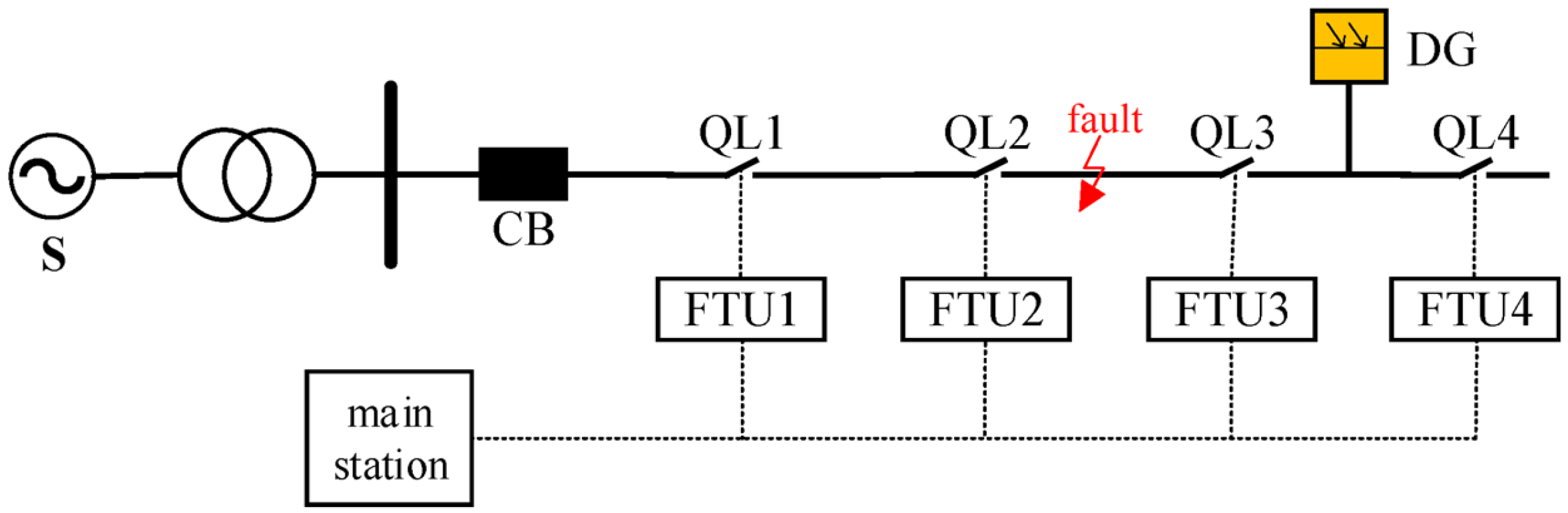
2.2. The Working Principle of Feeder Automation

The FA mode is mainly composed of the distribution main station, distribution sub-station, FTUs, communication systems, etc., and has the functions of remote signaling, remote measurement, remote control, and remote regulation. Through the two-way information exchange between the FTUs and the distribution main station, the system can process fault information in real time and collect the operation data of the distribution network, thereby optimizing the operation mode of the distribution network. When a fault occurs, the distribution main station can intelligently determine the fault location, send remote control signals to cut off the faulty equipment, quickly isolate the fault, and restore the power supply to the non-fault area. This mode can not only effectively deal with faults when they occur on the line but can also achieve centralized monitoring and management during the normal operation of the distribution network [23], as shown in Figure 1.

In the figure, CB is the circuit breaker at the line outlet, FTU1 to FTU4 are FTU devices, and QL1 to QL4 are sectionalizing switches controlled by the distribution terminal. When a fault occurs at the position, as shown in the figure, the following happens:

(1)

In the case of a transient fault, after the CB trips, it will automatically reclose after a certain period of time, and the power supply of the line will be restored.

(2)

In the case of a permanent fault, the CB will trip again after reclosing. The FTUs in the line will detect the fault current twice and send the fault information to the distribution main station. After receiving the information, the distribution main station will analyze the fault information and determine the fault location. If FTU2 is a “two-telemetry” device, the staff need to go to the site in a timely manner to operate the corresponding switch for fault isolation. If FTU3 is a “three-telemetry” device, it can automatically control the switch to open and quickly isolate the fault area. After QL2 and QL3 trip to isolate the fault, the CB is reclosed, and the DG in the network will continue to operate in parallel with the grid and participate in the power grid reconstruction after the fault, so as to restore the power supply to the non-fault area. If FTU3 is not configured for QL3, after the fault occurs, QL4 needs to act to isolate the fault. In this case, the DG is located within the fault area, and the fault isolation will lead to the disconnection of the DG from the distribution network, resulting in a waste of power resources.

In conclusion, the power outage time of the load and whether the DG is disconnected from the grid are closely related to the type, action time, and installation location of the FTU. Therefore, based on whether FTUs are configured between the load, DG, and the fault point, this paper analyzes the specific power outage loss costs of the load at various locations and the disconnection loss costs of the DG, aiming to achieve the optimal configuration of FTUs.

3. Mathematical Model for the Optimal Configuration of Distribution Terminals

3.1. Objective Function

The objective function of the mathematical model for the optimal configuration of FTUs is shown in Equation (1).

$$\min \left(C_{\mathrm{F}}+C_{\mathrm{M}}+C_{\mathrm{G}}\right)$$

(1)

In this equation, the objective function is obtained by adding the initial investment cost of the terminal $C_{\mathrm{F}}$, the power outage loss cost $C_{\mathrm{M}}$, and the disconnection cost of DG from the grid $C_{\mathrm{G}}$, which represents the minimization of the total investment cost.

3.2. Investment Cost of FTU Equipment

The investment cost of FTU equipment, $C_{\mathrm{F}}$, is shown in Equation (2).

$$C_F=\left(N_2{C}_{f2}+N_3{C}_{f3}\right){\displaystyle \frac{q{\left(1+q\right)}^p}{{\left(1+q\right)}^p-1}}$$

(2)

In this equation, $N_2$ is the number of “two-telemetry” terminal units, $N_3$ is the number of “three-telemetry” terminal units, $C_{f2}$ is the price of all equipment required for the construction of a single “two-telemetry” switch terminal, $C_{f3}$ is the price of all equipment required for the construction of a single “three-telemetry” switch terminal, q is the discount rate, and p is the service life of the terminal.

3.3. Load Power Outage Loss Cost

This section takes into account the influence of the installation location of FTUs on the scope of the fault area as well as the impact of the types of FTUs upstream and downstream of the fault area on the power outage time of loads inside and outside the area. A method is proposed to demarcate the area according to the location of FTUs and determine the power outage time of loads based on the types of FTUs.

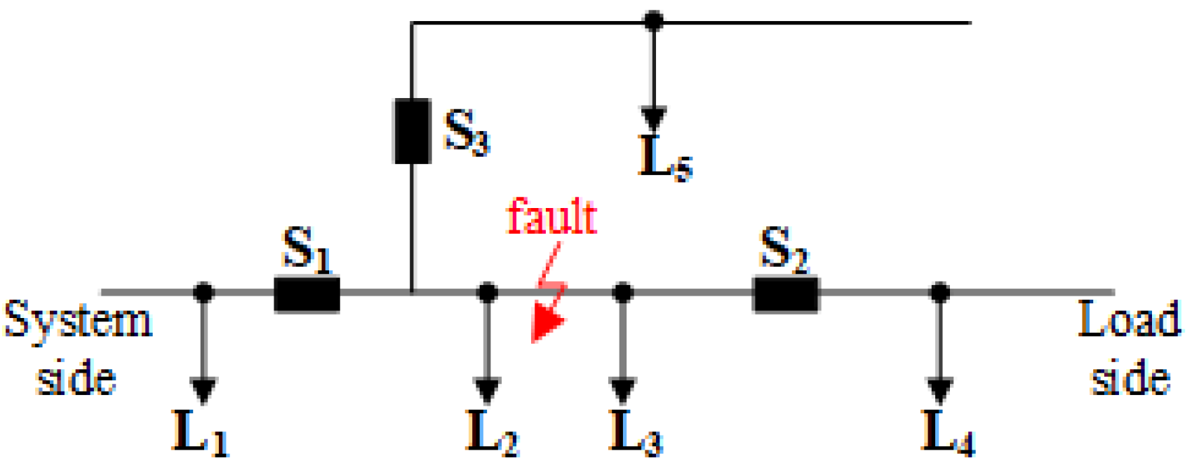
3.3.1. The Influence of FTU Location

The topology of the distribution system is shown in Figure 2. In the figure, L₁ to L₅ are loads, and S₁ and S₂ are FTUs. It is specified that the direction from the system power source to the line load is the positive direction.

According to whether there is an FTU between the fault point and the load and the relative position between the load and the FTU, the power outage time of the load after a fault occurs is divided into the following four categories:

Type 1: The load is located upstream of the fault point, and there is an FTU between the load and the fault point, such as with load L₁. The power outage time of load L₁ is related to the type of S₁.

Type 2: The load is located downstream of the fault point and there is an FTU between the load and the fault point, such as with load L₄. The power outage time of load L₄ is related to the type of S₂.

Type 3: There is no FTU between the load and the fault point, such as with loads L₂ and L₃. The power outage time of the loads is related to the types of S1 and S₂, which are the closest upstream and downstream points to the fault point.

Type 4: The load and the fault point are located on different feeder branches, such as with load L₅. The power outage time of L₅ is related to whether S₃ is installed and what type it is. If S₃ is not installed, there is no FTU between the load and the fault point, which is similar to Type 3; if S₃ is installed, according to the relative position between the load and the fault point, the load is located upstream of the fault point, which is similar to Type 1.

3.3.2. The Division of Fault Region and Non-Fault Region

According to the above four methods, the line between two adjacent FTUs is defined as a region. If there is a fault point within the region, this region is called a fault region. Based on this, the distribution network can be divided into three regions, namely the region upstream of the fault, the fault region, and the region downstream of the fault, as shown in Figure 3.

One can define t₁, t₂, and t₃ to represent the fault inspection time, fault isolation time, and power restoration time of the fault region, respectively. When there is an FTU between the load and the fault point and it is a “three-telemetry” type, the power outage time of this load is t₁. If the terminal is a “two-telemetry” type, the power outage time of this load is t₁ + t₂. When there is no FTU between the load and the fault point, the power outage time of the load is related to the types of FTUs upstream and downstream of the fault point. If both of the FTUs upstream and downstream of the fault point are of the “three-telemetry” type, the power outage time of the load is t₁ + t₃; if either the upstream or downstream FTU of the fault point is configured as a “two-telemetry” type, the power outage time of the load is t₁ + t₂ + t₃. In the topological structure of the distribution system, FTUs are usually installed at the beginning or end of the line. In this paper, it is assumed that all tie switches are installed with “three-telemetry” FTUs. After isolating the fault, the tie switches operate to ensure power supply to the non-fault regions.

According to the above analysis, the power outage times of each region are obtained as shown in Equation (3).

$$\{\begin{array}{c}{T}_s=V_1^{\mathrm{S}}\cdot t_1+\left(1-V_1^{\mathrm{S}}\right)V_1^{\mathrm{E}}\cdot \left(t_1+t_2\right)\hfill \\ T_g=\left[V_1^{\mathrm{S}}{V}_2^{\mathrm{S}}+V_1^{\mathrm{S}}\left(1-V_2^{\mathrm{S}}\right)\left(1-V_2^{\mathrm{E}}\right)\right]\cdot \left(t_1+t_3\right)\hfill \\ +\left[V_1^{\mathrm{S}}{V}_2^{\mathrm{E}}+V_1^{\mathrm{E}}{V}_2^{\mathrm{S}}+V_1^{\mathrm{E}}\left(1-V_2^{\mathrm{S}}\right)\left(1-V_2^{\mathrm{E}}\right)\right]\cdot \left(t_1+t_2+t_3\right)\hfill \\ T_x=V_2^{\mathrm{S}}\cdot t_1+\left(1-V_2^{\mathrm{S}}\right)V_2^{\mathrm{E}}\cdot \left(t_1+t_2\right)\hfill \end{array}$$

(3)

In this equation, $T_s$, $T_g$, and $T_x$, respectively, represent the power outage times of the region upstream of the fault, the fault region, and the region downstream of the fault. $V_1^{\mathrm{S}}$ and $V_1^{\mathrm{E}}$ are Boolean variables, which, respectively, indicate whether there is a “three-telemetry” FTU or a “two-telemetry” FTU in the region upstream of the fault. If there is, the value is taken as 1; otherwise, the value is taken as 0.

3.3.3. Cost of Power Outage Loss

The cost of power outage loss caused by the power outages of loads in each region due to faults in the distribution system is shown in Equation (4).

$$\begin{array}{c}{C}_{\mathrm{M}}={\displaystyle \sum _{i\in {\Omega }_i}{\displaystyle \sum _{s\in {\Omega }_s}{\lambda }_i{P}_s}{T}_s\left(P_s\right)C_{\alpha }\left(T_s\left(P_s\right)\right)}+{\displaystyle \sum _{i\in {\Omega }_i}{\displaystyle \sum _{g\in {\Omega }_g}{\lambda }_i{P}_g}{T}_g\left(P_g\right)C_{\alpha }\left(T_g\left(P_g\right)\right)}\\ +{\displaystyle \sum _{i\in {\Omega }_i}{\displaystyle \sum _{x\in {\Omega }_x}{\lambda }_i{P}_x}{T}_x\left(P_x\right)C_{\alpha }\left(T_x\left(P_x\right)\right)}\hfill \end{array}$$

(4)

In this equation, ${\Omega }_i$ is the set of fault points on the feeder; ${\lambda }_i$ is the occurrence probability of fault i; ${\Omega }_s$, ${\Omega }_g$ and ${\Omega }_x$ are, respectively, the sets of load types in the region upstream of the fault, the fault region, and the region downstream of the fault; $P_s$, $P_g$, $P_x$ are, respectively, the load amounts of a certain type of load in the region upstream of the fault, the fault region, and the region downstream of the fault; $T_s\left(P_s\right)$, $T_g\left(P_g\right)$, $T_x\left(P_x\right)$ are, respectively, the power outage times of a certain type of load in the region upstream of the fault, the power outage time of a certain type of load in the fault region, and the power outage time of a certain type of load in the region downstream of the fault; and $C_{\alpha }$ is the power outage loss cost per unit of electricity.

3.4. The Off-Grid Loss Cost of DG

The installation location of an FTU will directly affect the working status of DG when it is connected to or disconnected from the grid after fault isolation. If DG disconnects from the grid, it cannot participate in subsequent network reconfiguration or support power supply restoration, resulting in certain islanding loss costs and causing a waste of power resources. Therefore, in this section, a calculation method for the off-grid loss cost of the DG is proposed.

3.4.1. The Off-Grid Probability of DG

The change of the installation location of the FTU will lead to a change in the probability of a fault occurring in the region where the DG is located. Therefore, the total probability model is used to obtain the probability that a fault occurs in the region where the DG is located and the DG is disconnected from the grid.

$$p_{DG}={\displaystyle \sum _{j\in {\Omega }_j}{\lambda }_j}\cdot 1$$

(5)

In this equation, ${\Omega }_j$ is the set of faults occurring within the region where the DG is located.

3.4.2. Calculation of the Importance of DG Considering Capacity Size

The larger the capacity of the DG is, the greater the loss cost caused by the DG’s disconnection from the grid will be. Therefore, the importance weight of the DG is introduced, and the capacity size of the DG is used to measure the importance of the DG, as shown in Equation (6).

$$f\left(P\right)={\displaystyle \frac{5}{1+e^{-\left(P-5\right)}}}$$

(6)

In this equation, P represents the capacity of a single DG, with the unit of MW. Since the actual capacity of a single photovoltaic power generation unit generally does not exceed 5 MW, the parameter in the equation is set to 5.

3.4.3. The Off-Grid Loss Cost of DG

According to the above off-grid probability of DG, the importance weight of DG, and the capacity of DG, the off-grid cost of DG can be obtained, as shown in Equation (7).

$$C_{\mathrm{G}}={\displaystyle \sum _{G\in {\Omega }_G}{P}_{G}f\left(P_G\right)p\left(P_{\mathrm{G}}\right)}{C}_{\phi }$$

(7)

In this equation, ${\Omega }_G$ represents the set of DGs within the region, $P_{\mathrm{G}}$ represents the capacity of a single DG, $f\left(P_G\right)$ represents the importance weight of the DG, $p\left(P_{\mathrm{G}}\right)$ represents the off-grid probability of the DG, and $C_{\phi }$ represents the benchmark electricity price of the DG.

3.5. Constraint Conditions

3.5.1. The Average Service Available Index

In this paper, the Average Service Available Index (ASAI) is used to construct the power supply reliability constraint. According to the above method of dividing the fault regions, the power outage times of different regions are obtained, as shown in Equation (3). Based on the power outage times of different regions, the calculation method of ASAI is obtained, as shown in Equation (8).

$$\begin{array}{c}\mathrm{ASAI}={\displaystyle \frac{total power supply hours for users}{the number of power supply hours required by users}}\hfill \\ ={\displaystyle \frac{N\times 8760-\left[\left({\displaystyle \sum _{i\in {\Omega }_i}{\displaystyle \sum _{s\in {\Omega }_s}{\lambda }_i{N}_s}{T}_s\left(P_s\right)}+{\displaystyle \sum _{i\in {\Omega }_i}{\displaystyle \sum _{g\in {\Omega }_g}{\lambda }_i{N}_g}{T}_g\left(P_g\right)}+{\displaystyle \sum _{i\in {\Omega }_i}{\displaystyle \sum _{x\in {\Omega }_x}{\lambda }_i{N}_x}{T}_x\left(P_x\right)}\right)\right]}{N\times 8760}}\hfill \end{array}$$

(8)

In this equation, N is the total number of loads in the distribution network; 8760 is the number of hours in a year; $N_s$, $N_g$, and $N_x$ are, respectively, the numbers of loads in the section upstream of the fault, the fault section, and the section downstream of the fault.

3.5.2. Installation Constraints of FTUs

1.

Constraints on the Type of FTU at the Same Location

For each candidate installation location of an FTU, the number of different types of installed FTUs should not exceed 1. That is, the two-telemetry and three-telemetry FTUs cannot be installed simultaneously at the same location, as shown in Equation (9). This constraint ensures that the two-telemetry and three-telemetry FTUs are not installed concurrently, thereby reducing the economic cost.

$$V_e^1+V_e^2\le 1$$

(9)

In this equation, $V_e^1$ represents the installation of a three-telemetry FTU at location e, and $V_e^2$ represents the installation of a two-telemetry FTU at location e.

2.

Constraints on the Total Number of FTUs Installed in the Network

In the distribution network, if an FTU is not installed on a line, problems such as an expanded power outage scope and an increase in loss costs will occur. However, if there are too many FTUs on a line, it will lead to an increase in the FTU configuration cost and a waste of resources. Therefore, for a main line, the quantity constraint of the distribution terminals is as shown in Equation (10).

$$0<n_e\le n_{\max }$$

(10)

In this equation, n_e represents the number of FTUs installed on the line, and n_max represents the maximum number of FTUs that can be installed on the line. Its maximum value is determined according to actual planning.

3.5.3. Investment Cost Constraints

In the construction and renovation of distribution automation, the installation cost of the integrated primary and secondary equipment, including distribution terminals, should not exceed the total funds provided by the relevant department, as shown in Equation (11).

$$C_F\le C_{\max }$$

(11)

4. Model-Solving Process

PSO is a swarm intelligence algorithm that simulates the foraging behavior of birds. Its algorithm structure is simple, with few parameters, making it easy to understand and operate in practice. Moreover, it can quickly find a solution close to the optimal one. Through cooperation within the swarm, PSO can effectively avoid getting trapped in local optima. Additionally, it has excellent flexibility and can be applied to various types of problems, including continuous and discrete optimization problems.

In the process of the algorithm seeking the optimal solution, each potential optimal solution in every optimization process is regarded as a “bird” in the search space, which is called a “particle”. After evaluating the positions of all particles, the personal best position and the global best position are updated. This cycle is repeated until the expected target value is obtained or the maximum number of iterations is reached. The specific steps of the Particle Swarm Optimization (PSO) algorithm are described as follows [24,25,26,27].

Step 1: Initialize the particle population: Randomly initialize a swarm of particles in the search space, and the population size is N. Each particle represents a potential solution. The information of particle i is represented by a D-dimensional vector, and each particle has its position and velocity attributes. Among them, the position x_i of particle i can be expressed as $x={\left(x_{i1},x_{i2},\dots ,x_{iD}\right)}^T$, and the velocity can be expressed as $v={\left(v_{i1},v_{i2},\dots ,v_{iD}\right)}^T$.

Step 2: evaluate the fitness: calculate the fitness value of each particle according to the fitness value calculation equation to determine the performance of the particle in the search space.

Step 3: Update the personal best position (pbest): Compare the fitness value of each particle with the fitness value corresponding to its personal historical optimal position. If the current fitness value of the particle is smaller, then update the historical optimal position with the current position.

Step 4: Update the global best position (gbest): Compare the fitness value of each particle with the fitness value corresponding to the global optimal position. If the fitness value of the current particle is smaller, then update the global optimal position with the position of the current particle.

Step 5: update the velocity and position: use the velocity update Formula (12) and the position update Formula (13) to update the velocity and position of each particle.

$$\begin{array}{c}{V}_i^d\left(t+1\right)=\omega \cdot V_i^d\left(t\right)+c_1{r}_1\left(pbes{t}_i^d\left(t\right)-X_i^d\left(t\right)\right)\\ +c_2{r}_2\left(gbes{t}_i^d\left(t\right)-X_i^d\left(t\right)\right)\end{array}$$

(12)

$$X_i^d\left(t+1\right)=X_i^d\left(t\right)+V_i^d\left(t+1\right)$$

(13)

In these equations, $\omega$ is the inertia weight. This parameter enables the particle to maintain its motion inertia and reflects the degree of inheritance of the original velocity. $c_1$ and $c_2$ are the learning factors, $r_1$ and $r_2$ are random numbers, and d represents the dimension.

Step 6: Iteration: Repeat Steps 2 to 5 until the predetermined number of iterations is reached or other stopping conditions are met. After each iteration, the particle swarm gradually converges to the vicinity of the optimal solution in the search space.

Step 7: output the result: finally, output the found optimal solution, that is, the solution corresponding to the global best position.

5. Simulation Analysis

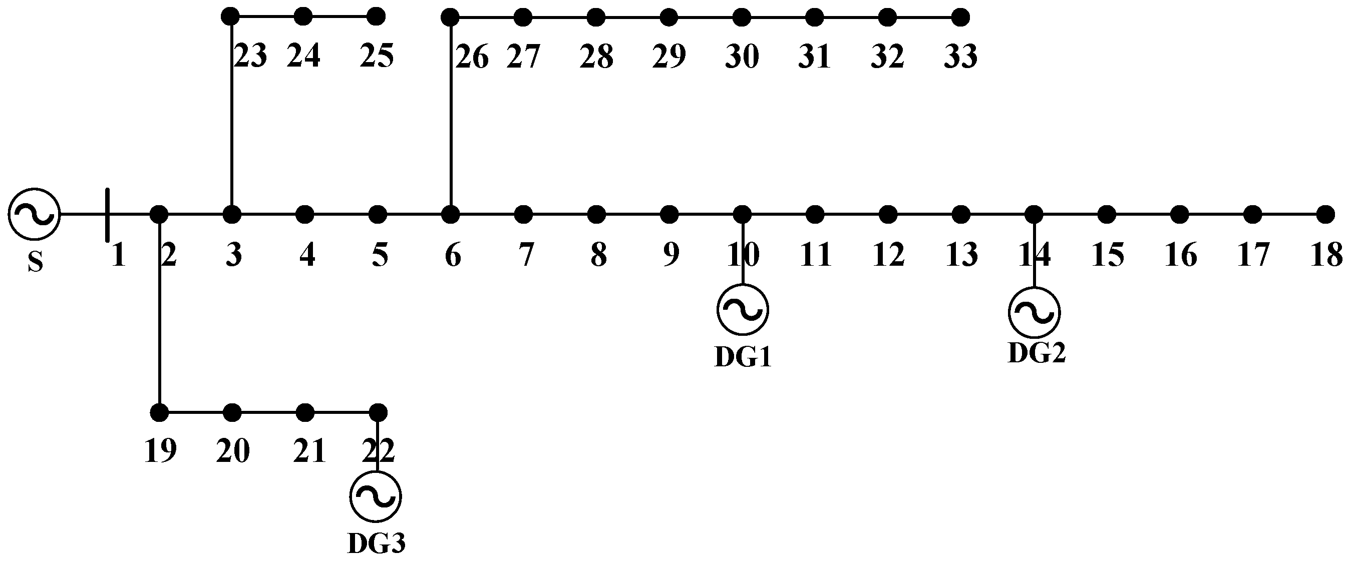
5.1. Scene Topology and Parameter Selection

The basic parameter settings of the PSO algorithm are as follows: the number of nodes is 33, the number of particles is 50, the maximum number of iterations is 100, the maximum velocity is 2, the inertia weight is 0.7, and both the individual learning factor and the social learning factor are 2. The network structure of the distribution network adopts the IEEE 33-node system, as shown in Figure 4. The numbers “2–33” represent the load nodes. The preset positions of FTUs are at each node. The installation costs of the two-telemetry and three-telemetry devices are 19,000 yuan per set and 55,000 yuan per set, respectively. The discount rate is set at 10%, the service life of the equipment is calculated as 20 years, the unit power outage loss is 11.7 yuan/(kW·h), and the minimum average power supply availability given by the system is 99.450%. The fault inspection time, fault isolation time, and fault recovery time are 3000 s, 1800 s, and 28,800 s, respectively [18]. The capacities of DG1, DG2, and DG3 are 380 kW, 650 kW, and 250 kW, respectively, and the off-grid cost is 200 yuan/(kW·h).

5.2. Analysis of Computational Examples

To verify the accuracy of the method proposed in this paper, three computational examples were designed for comparative analysis on MATLAB 2024. Computational Example 1 is the optimal configuration when only two-telemetry devices are deployed for the IEEE 33-node system; Computational Example 2 is the optimal configuration when only three-telemetry devices are deployed for the IEEE 33-node system; Computational Example 3 is the optimal configuration of both two-telemetry terminals and three-telemetry terminals for the IEEE 33-node system.

5.2.1. Computational Example 1

Considering the installation of only two-telemetry devices at the nodes of the IEEE 33-node system, the optimized configuration obtained under the condition of satisfying the constraints is shown in

Table 1. Full two-way remote configuration plan.

Node Number	Configuration Scheme	ASAI
2, 5, 10, 19, 24, 27, 28, 31	install two-telemetry device	94.48%
the other nodes	do not install

The cost of the optimal installation configuration is 721,373.26 yuan.

.

5.2.2. Computational Example 2

Considering the installation of only three-telemetry devices at the nodes of the IEEE 33-node system, the optimized configuration obtained under the condition of satisfying the constraints is shown in

Table 2. Full three-way remote configuration plan.

Node Number	Configuration Scheme	ASAI
3, 9, 11, 12, 19, 22, 26, 31	install three-telemetry device	94.08%
the other nodes	do not install

The cost of the optimal installation configuration is 565,230.04 yuan.

.

5.2.3. Computational Example 3

The optimal configuration of two-telemetry and three-telemetry devices at the nodes of the IEEE 33-node system was found, and the optimized configuration obtained under the condition of satisfying the constraints is shown in the

Table 3. Optimized configuration of two-way and three-way remote configuration plan.

Node Number	Configuration Scheme	ASAI
1, 3, 5, 6, 9, 11, 13, 21, 26, 27	install two-telemetry device	99.56%
7, 23, 29	install three-telemetry device
the other nodes	do not install

The cost of the optimal installation configuration is 657,882.04 yuan.

.

Comparing the above three scenarios, in Scenario 1, the configuration cost obtained by optimizing with the preset installation of “two-telemetry” terminals at all nodes is the highest among the three scenarios, and the ASAI does not meet the given minimum ASAI requirement. In Scenario 2, the configuration cost obtained by optimizing with the preset installation of “three-telemetry” terminals at all nodes is the lowest, but the ASAI also fails to meet the given minimum ASAI requirement. In Scenario 3, both “two-telemetry” and “three-telemetry” terminals are configured, and the derived configuration scheme not only meets the minimum ASAI requirement specified by the system, but also ensures economic efficiency, thus having application value in practical engineering projects.

The optimal terminal configurations of the “two-telemetry” and “three-telemetry” devices derived from Scenario 3 are shown in Figure 5.

6. Conclusions

In this paper, considering the influence of the location and types of FTUs on the load outage time within the fault area and the off-grid loss cost caused by the disconnection of distributed photovoltaics in the fault area, an optimal configuration method for FTUs is proposed. The research constructs an optimal configuration model with power supply reliability and FTU installation cost as constraint conditions with the goal of minimizing the sum of the initial installation cost of FTUs, load outage loss, and photovoltaic off-grid cost. The following conclusions are drawn in this paper:

(1)

The influence of FTUs of different types and locations on the load outage time was analyzed. Based on this, a new definition method for the load outage time is proposed when there is no FTU between the load and the fault point, thus making the calculation of the load outage time more accurate. The fault area and non-fault area were divided according to the installation location of FTUs, and then the load outage loss models for different areas were established.

(2)

A photovoltaic off-grid loss model was established, which makes the FTU configuration model more comprehensive and the optimization results more reasonable. By introducing the total probability model, the off-grid probability of distributed photovoltaics under fault conditions was calculated, and the importance weight was determined according to the capacity of distributed photovoltaics, thus constructing the photovoltaic off-grid loss model.

(3)

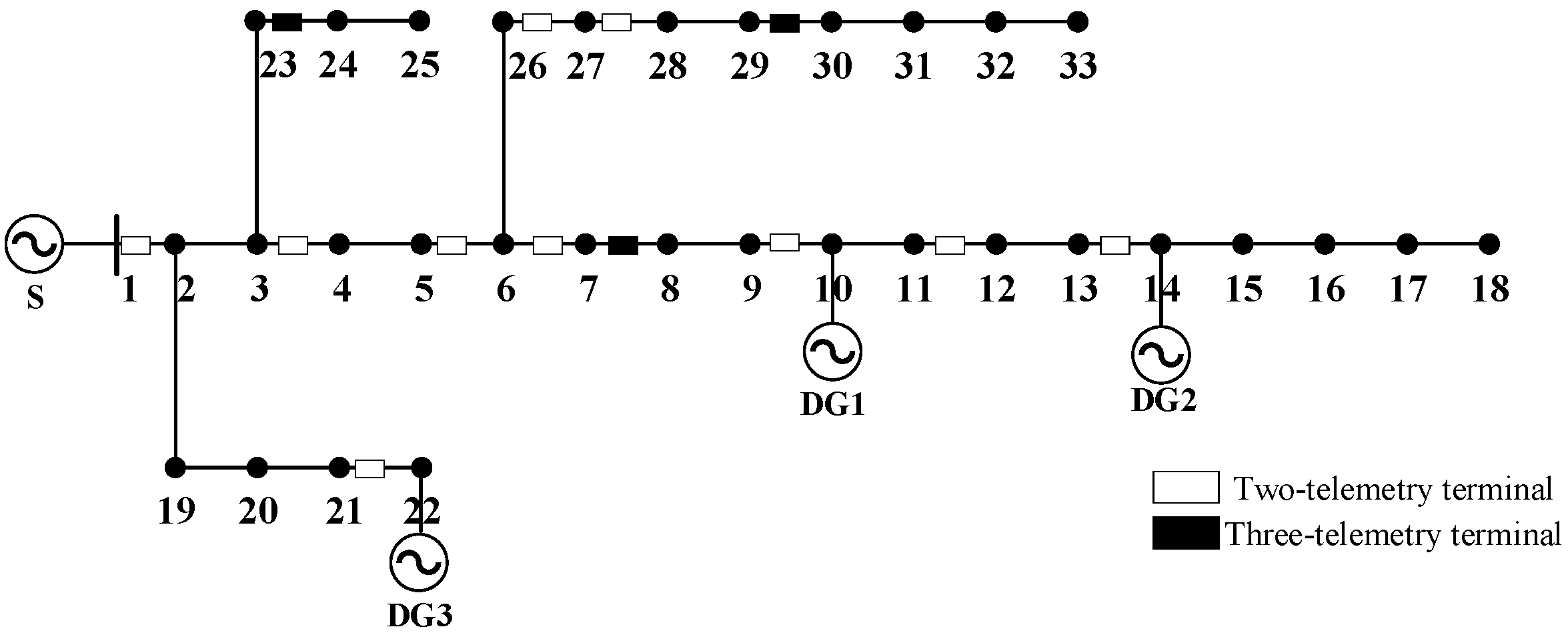
An optimization model was constructed with the average power supply availability rate and the installation cost and quantity of FTUs as constraint conditions. By using the PSO algorithm, and under the premise of considering the constraint conditions, the optimal configuration scheme of FTUs for the IEEE 33-node distribution network was solved.

References

1. Wang, W. Practical Fault Locating Technology for Medium and High Voltage Distribution Network Based on Fault Record. Master’s Thesis, Zhejiang University, Hangzhou, China, 2024. [Google Scholar]
2. Keshavarz, A.; Dashti, R.; Deljoo, M.; Shaker, H.R. Fault location in distribution networks based on SVM and impedance-based method using online databank generation. Neural Comput. Appl. 2022, 34, 2375–2391. [Google Scholar] [CrossRef]
3. Zeng, R.; Zhang, Z.; Wu, Q. Fault location scheme for multi-terminal transmission line based on frequency-dependent traveling wave velocity and distance matrix. IEEE Trans. Power Deliv. 2023, 38, 3980–3990. [Google Scholar] [CrossRef]
4. Khatib-Tohidkhaneh, F.; Mohammadi-Hosseininejad, S.M.; Saberi, H. A probabilistic electric power distribution automation operational planning approach considering energy storage incorporation in service restoration. Int. Trans. Electr. Energy Syst. 2020, 30, 398–409. [Google Scholar] [CrossRef]
5. Huang, Z.; Qin, F.; Zhu, G.; Wang, D.; Yang, M. Fast Fault Location Method for Complex Active Distribution Network Based on Improved Impedance Method. Tech. Autom. Appl. 2023, 42, 80–84. [Google Scholar]
6. Elgamasy, M.M.; Elezzawy, A.I.; Kawady, T.A.; Elkalashy, N.I.; Elsadd, M.A. Tracing passive traveling surge-based fault management control scheme in unearthed distribution systems. Electr. Eng. 2024, 106, 5603–5624. [Google Scholar] [CrossRef]
7. Tang, J.; Yin, X.; Zhang, Z.; Yang, C.; Ye, L.; Qi, X.W. Survey of fault location technology for distribution networks. Electr. Power Autom. Equip. 2013, 33, 7–13. [Google Scholar]
8. Hu, L.; Wang, L.; Zheng, W.; Sun, K.; Hu, Z.; Gao, Q.; Sun, W. Optimal planning of switch points based on comprehensive analysis of grid structure. Power Syst. Clean Energy 2019, 35, 28–35. [Google Scholar]
9. Liu, B.; Zhang, X.; Wang, Y.; He, L.; Wang, Z.; Du, M. Optimal layout method of distribution terminals considering the whole process of feeder automatic fault handling. Power Syst. Prot. Control 2023, 51, 97–107. [Google Scholar]
10. Li, S.; Wang, Z.; Xu, W.; Wu, J. Practical optimization models and methods for mv feeder segmentation strategies. Power Syst. Technol. 2022, 46, 765–777. [Google Scholar] [CrossRef]
11. Li, S.; Wang, Z.; Zeng, H.; Li, W.; Wang, D. Discussion on lean planning and management improvement strategies for first-class distribution networks. Power Syst. Prot. Control 2021, 49, 165–176. [Google Scholar]
12. Xu, C. The Real-Time Performance of Communication Network in Distributed Intelligent Feeder Automation System. Master’s Thesis, Shanong University of Technology, Zibo, China, 2012. [Google Scholar]
13. Zhang, J.; Tang, J.; Cao, H.; Gao, C.; Yu, T. Life cycle cost model and intelligent optimization of distribution automation terminal unit. Electr. Meas. Instrum. 2020, 57, 81–89. [Google Scholar]
14. Wang, X. Research on Distribution Automation System Planning for Power Supply Reliability. Autom. Appl. 2023, 64, 200–202. [Google Scholar]
15. Liu, J.; Cheng, H.; Zhang, Z. Planning of terminal unit amount in distribution automation systems. Autom. Electr. Power Syst. 2013, 37, 44–50. [Google Scholar]
16. Liu, J.; Lin, T.; Zhao, J.; Wang, P.; Su, B.; Fan, X. Specific planning of distribution automation systems based on the requirement of service reliability. Power Syst. Prot. Control 2014, 42, 52–60. [Google Scholar]
17. Chen, R.; Li, X.; Chen, Y. Type and site selection model of distribution terminals and switches adaptive to different network architectures. Autom. Electr. Power Syst. 2022, 46, 151–160. [Google Scholar]
18. Sun, L.; Yang, H.; Ding, M. Mixed integer linear programming model of optimal placement for switching devices in distribution system. Autom. Electr. Power Syst. 2018, 42, 87–95. [Google Scholar]
19. Farajollahi, M.; Fotuhi-Firuzabad, M.; Safdarian, A. Optimal placement of sectionalizing switch considering switch malfunction probability. IEEE Trans. Smart Grid 2019, 10, 403–413. [Google Scholar] [CrossRef]
20. Sun, L.; Yang, Y.; Zhang, C.; Chen, H.; Wang, T.; Jiao, A. Distribution terminal optimal design for distributed generation accessing distribution network. Acta Energiae Solaris Sin. 2021, 42, 120–125. [Google Scholar]
21. Liu, J.; Pan, J.; Zhang, S. Optimization of distribution terminal selection considering load and dg randomtiming characteristics. Mech. Electr. Eng. Technol. 2020, 49, 154–157. [Google Scholar]
22. Zhao, H.; Ding, J.; Yang, M.; Wang, C.; Qu, G.; Gong, J. Research on voltage and reactive power of system with 10 million kilowatts wind and photovoltaic power. Renew. Energy Resour. 2020, 49, 154–157. [Google Scholar] [CrossRef]
23. Li, G. Research on Faulted Section Location Method of Distribution Network Based on Feeder Automation Information. Master’s Thesis, Shandong University, Jinan, China, 2021. [Google Scholar]
24. Gao, J.; Diao, N.; Hou, X.; Sun, Y.; Xue, X. Reactive Power Optimization of Active Distribution Network Based on Improved Particle Swarm Algorithm. Tech. Autom. Appl. 2024, 43, 19–23. [Google Scholar]
25. Fu, Z. MLR-MPSO-based Arrangement Optimization of Monitoring Points in Transmission Networks. Electr. Eng. 2024, 19, 40–45. [Google Scholar]
26. Xiong, R.; Zhao, L.; Zhang, Y. Fault Location of Active Distribution Network Based on GWO-PSO Algorithm. Proc. CSU-EPSA 2024, 1–10. [Google Scholar]
27. Sun, S. A Method for Solving Large Scale Multiobjective Optimization Problems Based on Particle Swarm Optimization. Master’s Thesis, China University of Mining and Technology, Beijing, China, 2023. [Google Scholar]
Figure 1. Feeder automation system architecture.
Electronics 14 02117 g001
Figure 2. Topology of the distribution system.
Electronics 14 02117 g002
Figure 3. Classification of fault areas.
Electronics 14 02117 g003
Figure 4. IEEE 33 node distribution network topology.
Electronics 14 02117 g004
Figure 5. FTU final configuration scheme.
Electronics 14 02117 g005