Article

Enhancing Indoor Positioning with GNSS-Aided In-Building Wireless Systems

by
Shuya Zhou
1,2,
Xinghe Chu
1,2 and
Zhaoming Lu
1,2,*
1
School of Information and Communication Engineering, Beijing University of Posts and Telecommunications, Beijing 100876, China
2
Beijing Laboratory of Advanced Information Networks, Beijing 100876, China
*
Author to whom correspondence should be addressed.
Electronics 2025, 14(10), 2079; https://doi.org/10.3390/electronics14102079
Submission received: 18 April 2025 / Revised: 16 May 2025 / Accepted: 19 May 2025 / Published: 21 May 2025
(This article belongs to the Special Issue Mobile Positioning and Tracking Using Wireless Networks)

Abstract

:
Wireless indoor positioning systems are challenged by the reliance on densely deployed hardware and exhaustive site surveys, leading to elevated deployment and maintenance costs that limit scalability. This paper introduces a novel positioning framework that enhances the existing In-Building Wireless (IBW) infrastructure by retransmitting Global Navigation Satellite System (GNSS) signals. Pseudorange residuals extracted from raw GNSS measurements, when mapped against known cable lengths, facilitate anchor identification and precise ranging. In parallel, directional and inertial measurements are derived from the channel state information (CSI) of cellular reference signals. Building upon these observations, we develop a Hybrid Adaptive Filter-Graph Fusion (HAF-GF) algorithm for high-precision positioning, wherein the adaptive filter modulates observation noise based on Line-of-Sight (LoS) conditions, while a factor graph optimization over multiple positional constraints ensures global consistency and accelerates convergence. Ray tracing-based simulations in a complex office environment validate the efficacy of the proposed approach, demonstrating a 30% improvement in positioning accuracy and at least a threefold increase in deployment efficiency compared to conventional methods.

1. Introduction

Indoor positioning offers enormous potential due to the rapid growth in internet of things, mobile computing, and smart wearables, wherein location-based services have become essential for both personal and industrial applications. However, despite this rising demand, achieving high-precision indoor positioning remains difficult [1]. Although Global Navigation Satellite Systems (GNSSs) excel in outdoor positioning, their performance indoors is compromised by significant signal attenuation and obstruction from structural elements such as walls and floors.
Over the past decades, substantial studies have been made in indoor positioning systems (IPSs). Many existing approaches depend on installing multiple specialized signal transmitters, such as Bluetooth Low Energy (BLE) [2], Wi-Fi [3], and Ultra-WideBand (UWB) [4]. Furthermore, GNSS-inspired systems like Pseudolites [5] and Repealites [6] have been developed to deliver satellite signals within buildings. Pseudolites utilize ground-based transmitters to emit GNSS-compatible signals with known spatial and temporal references, whereas Repealites operate by receiving authentic GNSS signals outdoors and subsequently amplifying and re-radiating them indoors. Receivers estimate their positions by measuring the pseudoranges to multiple transmitters, following the same principle employed by conventional GNSS.
Nonetheless, these methods often struggle with issues such as severe multipath propagation and frequent signal blockages, necessitating the use of dedicated transmitters to facilitate various lateration or angulation measurements, or to generate distinctive fingerprints. This requirement inevitably drives up costs and complicates long-term maintenance. In addition, GNSS-like solutions are susceptible to the near-far effect, where signals from remote transmitters degrade into noise and lead to detection failures [7].
In an effort to overcome the limitations imposed by purpose-built infrastructure, researchers have increasingly turned to IPSs that harness existing radio frequency (RF) signals from in-building cellular systems [8]. These In-Building Wireless (IBW), such as 4G Long-Term Evolution (LTE) and emerging 5G New Radio (NR), are already widely deployed to provide continuous indoor coverage. By repurposing these existing assets, indoor positioning can be achieved in a more cost-effective manner without requiring extensive new installations [9,10].
Recent investigations in this area have predominantly focused on exploiting 5G technology—characterized by large-scale antenna arrays and high-capacity, low-latency communication—to enhance localization performance. Various methodologies have been examined that leverage reference signals from either cellular uplink or downlink transmissions to extract geometric parameters such as Time of Arrival (ToA) [11], Time Difference of Arrival (TDoA) [12], and Direction of Arrival (DoA) [13], or employ deep learning techniques to extract advanced features from reference signals for finer-grained positioning [14,15]. Alternatively, fingerprinting techniques that compare observed signal strength patterns with pre-established templates have been employed [16,17,18]. These approaches often require constructing and continuously updating extensive fingerprint databases, which is labor intensive and challenging to maintain.
In response to these challenges, we propose a novel IPS that integrates GNSS signals with IBW. Our approach introduces outdoor satellite signals into indoor spaces through the already-installed IBW infrastructure, allowing indoor devices to capture both cellular and GNSS measurements without compromising network service. This solution leverages the extensive and ubiquitous nature of cellular coverage provided by densely distributed cell towers and indoor units, thereby enabling scalability across large regions. Additionally, by predominantly basing localization on geometric measurements rather than fingerprinting, our method promises superior adaptability to environmental changes and broader applicability across different equipment platforms.
The key contributions of this paper are summarized as follows:
  • We present a novel localization architecture that integrates GNSS and IBW systems by repurposing existing distributed antennas as GNSS retransmitters, enabling anchor identification and accurate ranging under LoS conditions. Combined with DoA and inertial cues extracted from downlink CSI, the system supports high-precision positioning without the deployment of multiple signal sources.
  • A robust LoS/NLoS detection mechanism is introduced, leveraging signal strength disparities and CSI dynamics. This is incorporated into a Hybrid Adaptive Filter–Graph Fusion (HAF-GF) algorithm, which integrates real-time adaptive filtering with factor graph optimization. The LoS confidence score adaptively modulates measurement noise and influences graph weights for enhanced robustness and convergence.
  • System-level simulations using 3GPP-compliant signals and ray-tracing in a complex office environment demonstrate 0.69 m accuracy at the 90th percentile, yielding a 30% improvement over baseline fusion algorithms. The proposed system achieves high precision with minimal infrastructure and strong adaptability to varying indoor conditions.
The remainder of this paper is organized as follows. Section 2 reviews related work. Section 3 introduces the proposed system structure integrating GNSS and IBW. Section 4 presents the available positional measurements of this system from both GNSS and cellular signals. The HAF-GF localization algorithm is explained in Section 5. The experimental results are analyzed in Section 6. Finally, Section 7 concludes this work and discusses final remarks.

2. Related Work

2.1. Indoor GNSS Solutions

Early work on retransmitting outdoor GNSS signals for indoor positioning dates back to 2004 [19], where an architecture was proposed comprising an external GNSS antenna and a set of switching modules to relay signals indoors. Upon collecting sufficient sequential range measurements, TDoA techniques were employed for position estimation. Subsequently, the time-delayed repeating method was introduced in [20,21], where each indoor retransmission antenna broadcasted a common satellite signal with a unique delay exceeding two code chips. This scheme mitigated signal interference and enabled real-time dynamic positioning using instantaneous measurements. A more advanced architecture was proposed in [22], wherein the signals from individual satellites were extracted from the received GNSS stream before being forwarded through indoor transmitters. This method achieved positioning accuracies of 1.0 m and 1.2 m under static and dynamic conditions, respectively. In [6], the time-delayed repeating framework was extended to scenarios with multiple outdoor GNSS antennas. A closed-form solution was derived to compute the receiver’s position based on the measured time-of-flight from multiple repeaters, achieving an accuracy of 2.7 m. More recently, ref. [23] introduced a differential GNSS-based indoor positioning technique requiring at least seven repeaters. The receiver performs carrier-phase measurements using signals from multiple repeaters. By selecting a reference repeater, phase differences between pairs of repeaters are computed, and the differenced phase measurements across consecutive epochs are used to infer the user’s location.

2.2. IBW-Based Positioning

IBW-based positioning approaches commonly rely on features extracted from downlink reference signals, such as the Received Signal Strength Indicator (RSSI) and Reference Signal Received Power (RSRP). Methods such as sequence-based correlation with pre-constructed templates have been employed for localization [16]. In [17], RSSI measurements and physical cell identifiers, collected via smartphones, were utilized to construct sequence fingerprints for vehicular positioning within tunnel environments. A centralized software-defined networking (SDN) platform was proposed in [24] to manage indoor femtocells, supporting multiple network-level optimizations including K-nearest neighbor (KNN)-based fingerprinting localization. Similarly, a weighted KNN-based enhancement of the cell-ID approach was presented in [18] and evaluated across a range of indoor scenarios. Machine learning methods have also gained traction in this domain. For instance, ref. [25] explored the use of neural networks and random forests to estimate user location under NLoS conditions by leveraging the best-received reference signal beam power in 5G networks. In [26], deep neural networks were applied to downlink cellular signals from IBW systems for pedestrian localization. Meanwhile, ref. [27] proposed a hybrid approach integrating Wi-Fi fingerprints with IBW-defined sub-regions to enhance localization performance. Owing to the relatively uniform distribution of RF energy in such systems, the achieved localization accuracy typically remains within 10 m.

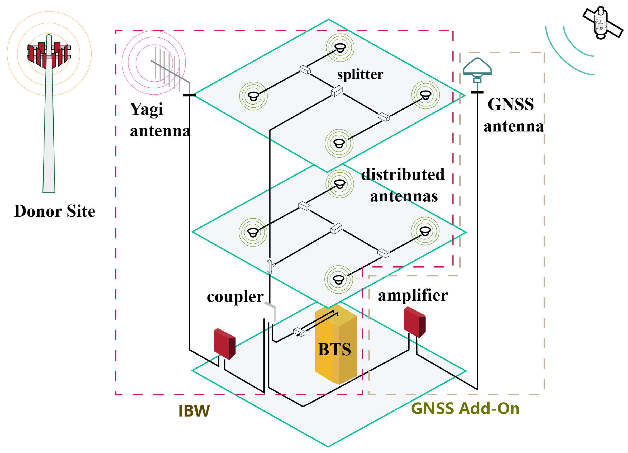
3. Proposed System Structure

The conceptual framework of our localization system is depicted in Figure 1. In this illustration, we consider a typical IBW structure, specifically a passive distributed antenna setup that includes a signal source, couplers, splitters and dome antennas mounted on the ceiling.

3.1. Infrastructure Segment

Originally, the transmitting segment includes a cellular signal source from either a Yagi antenna that captures signals from a remote donor site—routing them through a bi-directional amplifier—or a direct feed from a Base Transceiver Station (BTS). After signal distribution via the couplers and splitters, the dome antennas broadcast the cellular signal throughout the indoor environment. Our primary modification to this existing IBW involves installing GNSS receiving antennas in outdoor areas; these antennas are connected to the couplers positioned between each RF signal source and the IBW head-end unit. Since the satellite signals are inherently below the thermal noise floor and are merely carried passively over the system, this dual-purpose signal transmission does not interfere with the original cellular coverage function of the IBW. As a result, satellite signals can be seamlessly integrated into the existing IBW framework through minimal add-ons, enabling the distributed antennas to emit a composite signal that includes both cellular service signals and amplified replicas of outdoor GNSS satellite signals.

3.2. User Segment

The receiving segment comprises standard GNSS- and cellular-capable devices such as smartphones, connected vehicles, or internet-of-things terminals equipped with integrated chipsets and antennas. These devices are further expected to support raw signal acquisition to extract essential observables such as pseudoranges, Doppler shifts, and CSI packets. They receive time-delayed replicas of the same GNSS and cellular signals, re-radiated via multiple indoor distributed antennas. Once the dominant signal source is identified, the device extracts positioning observables from the composite signal stream, enabling indoor localization without hardware modifications.

3.3. Anchor Modeling and Signal Characterization

Since components in IBW are passive, the signals transmitted through different indoor distributed antennas are identical at the data level. Embedding unique digital identifiers into the signals emitted by each antenna is therefore impractical. Instead, each distributed antenna effectively serves as a GNSS anchor by introducing a distinct propagation delay, determined by the length of the coaxial cable connecting it to the outdoor GNSS antenna. As a result, the receiver captures multiple copies of the same satellite signal from different anchors, each arriving at slightly different times.
Given the civil coarse/acquisition (C/A) code’s 1.023-Mcps chip rate and its corresponding code period of 1023 chips, it is statistically unlikely for a signal to arrive with a delay greater than one full code period (approximately 293 m). Thus, only the signal from the nearest anchor significantly contributes to the correlation peak, while copies from more distant anchors manifest primarily as multipath-like background noise. Benefiting from the low skewness and high kurtosis characteristics of Line-of-Sight propagation, the influence of these secondary signals on the main lobe of the Gold code autocorrelation function is minimized. This characteristic facilitates the identification of specific anchors and mitigates the near-far effect typically encountered in indoor propagation. Moreover, the physical separation and distinct cable delays between antennas, especially when deployed across multiple rooms or floors, further reduce the likelihood of signal overlap, thereby enhancing spatial separability and suppressing background interference.

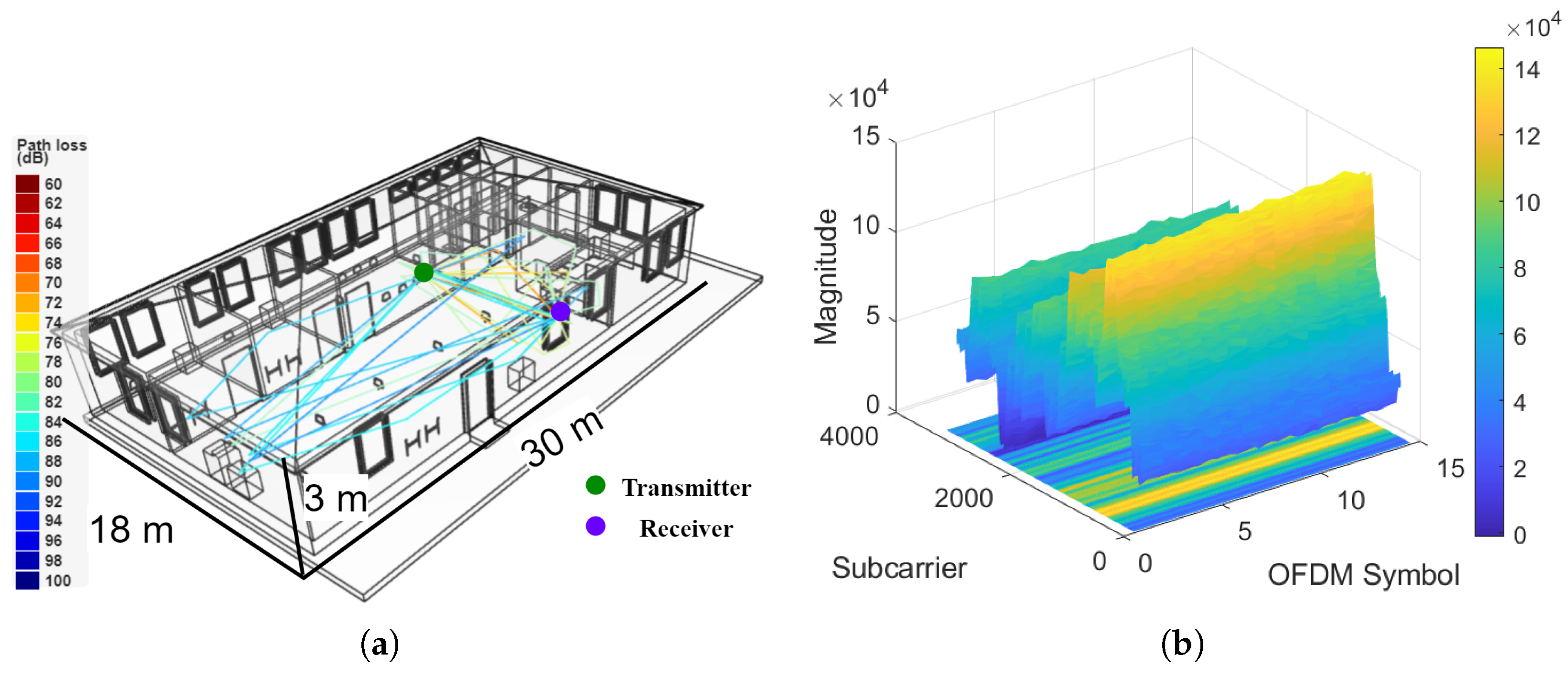
4. Localization Measurements of the System

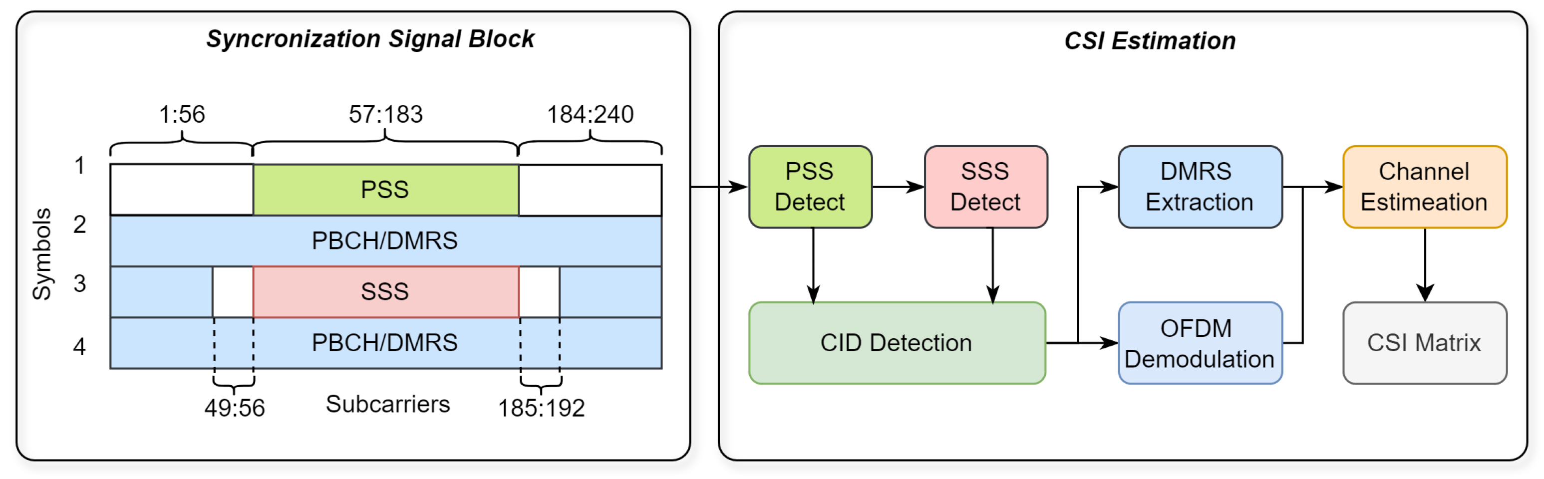
4.1. Anchor Identification and ToA Estimation

The proposed architecture utilizes raw GNSS observations to facilitate anchor identification and determine ToA to the serving anchor. The process begins by separating pseudorange and pseudorange rate into outdoor and indoor contributions.
When the delay lock loop within the signal processor identifies the point of maximum correlation with a satellite signal via relay through the IBW, it generates an observation corresponding to the code phase, effectively marking the signal’s transmit time t T relative to the local receive time t R . Owing to clock offsets relative to GNSS system time, these can be expressed as t T = t s ( i ) + δ t s ( i ) for the ith satellite, and t R = t u + δ t u for the user receiver, where t s ( i ) and t u denote the satellite and user clock times in GNSS time, respectively, and δ t s ( i ) and δ t u represent their corresponding clock biases. The pseudorange observable is then given by the time interval multiplied by the speed of light, expressed as ρ = c · ( ( t u + δ t u ) ( t s ( i ) + δ t s ( i ) ) ) . Based on the complete signal propagation trajectory, the total pseudorange can be conceptually partitioned into two distinct components: the outdoor pseudorange and indoor pseudorange.
The outdoor component, observed between the outdoor GNSS antenna and satellite i, denotes the distance traversed by the signal from the satellite to the rooftop GNSS antenna through atmospheric propagation,
ρ out i = r s i r o δ t s i + δ t iono , trop i + ϵ ρ out i ,
where r s i and r o represent the three-dimensional position vector of the ith satellite and the outdoor GNSS antenna in the Earth-Centered, Earth-Fixed (ECEF) coordinate system, and δ t iono , trop refers to the ionospheric and tropospheric delays. For notational convenience, all time bias terms are implicitly multiplied by the speed of light and expressed as distances. After compensating for the atmospheric delays with differential GNSS technique, all other sources of error induced by propagation path residual or imprecise ephemeris are collectively denoted by ϵ ρ out .
The indoor pseudorange ρ in n is essentially the propagation distance from the outdoor antenna to the nth indoor distributed antenna via coaxial cabling, followed by its transmission through the indoor air interface to the User Equipment (UE). Besides the receiver instrument delay and measurement noise represented by ϵ ρ in , it encompasses the receiver clock bias δ t u , indoor cable electrical length d cable , and propagation distance of the air interface,
ρ in n = d cable n + r a ( n ) r u + δ t u + ϵ ρ in ,
where r a ( n ) represents the location of the nth indoor distributed antenna, and r u the location of the UE.
The carrier tracking loop, governed by the numerically controlled oscillator, reveals the frequency offset between the received and expected signal frequencies. This discrepancy arises primarily from Doppler effects induced by the relative motion of both the satellite and receiver, as well as from clock instabilities on either end. The pseudorange rate is calculated by multiplying the observed Doppler shift by the negative of the carrier wavelength. Similar to the pseudorange, the pseudorange rate can be partitioned into indoor and outdoor components by taking the time derivatives of Equations (1) and (2). This decomposition relies on the assumption that the temporal variation of ionospheric and tropospheric delays, along with other minor error sources, remains sufficiently small to be ignored:
ρ ˙ out i = r s i r o δ t s i + δ t iono , trop i + ϵ ρ out i t
= v s i 0 fixed outdoor antenna · I out i δ f s i , ρ ˙ in n = d cable n + r a i r u + δ t u + ϵ ρ in t = 0 fixed distributed antenna v u · I in n + δ f u ,
where we use v s i and v u to denote the velocities of the satellite and the receiver, respectively, and δ f s i , δ f u to signify the clock drift in meters per second for the satellite and receiver. Additionally, I out ( n ) = r s ( i ) r o r s ( i ) r o is the direction vector from the outdoor antenna to the satellite, while I in ( n ) = r a ( n ) r u r a ( n ) r u is the direction vector of the indoor air interface from the receiver to the distributed antenna.
The cumulative receiver clock bias term, δ t u in Equation (2), can quickly overshadow other relevant components due to the frequency drift inherent in the receiver’s local oscillator over time. To address the challenge, the indoor pseudorange rate from Equation (4), which provides an imperfect yet valuable approximation of the actual clock drift, can be integrated over time to effectively compensate for the internal clock bias,
Δ ρ in = ρ in n t ρ ˙ in n d t δ t u 0 = d cable n + r a ( n ) r u + t v u · I in n d t + ϵ ρ in ,
where δ t u 0 represents the initial clock bias of the receiver which can be pre-calibrated since the pseudorange residual simplifies solely to the initial clock bias when measured outdoors.
Assuming the UE velocity v u is small, as is often the case in indoor environments, the calculated pseudorange residual can be regarded as the combined effect of the cable’s electrical length and the air interface distance. Hence, the antenna identity N AID and ranging estimation d ( N AID ) can be derived by correlating the indoor pseudorange residuals with the actual electrical lengths of the indoor cables corresponding to the N anchor nodes,
N AID = min n Δ ρ in d cable n , n 1 , N , d ( N AID ) = Δ ρ in d cable N AID .
Differentiating between signal source antennas and performing ranging estimation relies on the fundamental premise that differences in cable lengths among various antennas substantially exceed the corresponding over-the-air distances. With an appropriate layout design, anchor identification can be effectively employed for localization within partitioned sub-areas, such as across different floors or among discrete rooms on the same level.

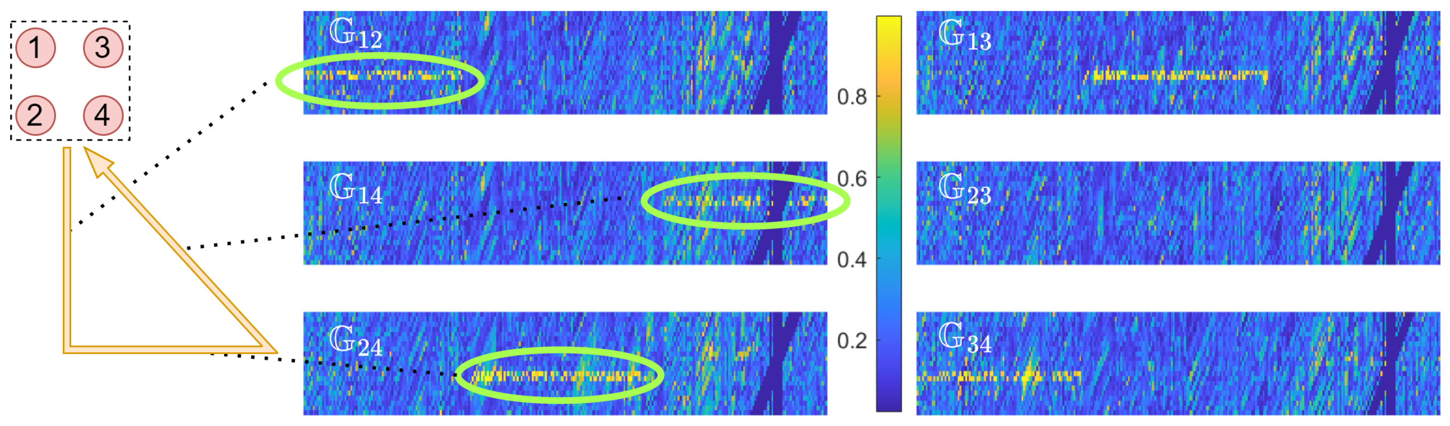
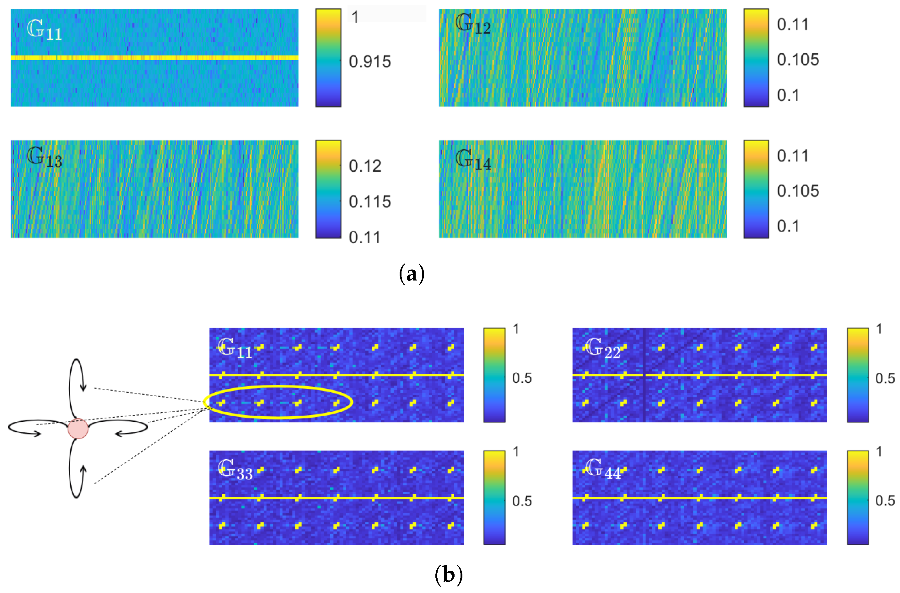
4.2. NR CSI Acquisition and DoA Estimation

Once the serving anchor is identified and ToA measurements are obtained, their integration with both the azimuth and elevation angles of arrival enables the determination of the position of the UE. We exploit the CSI derived from the Demodulation Reference Signal (DMRS) in the downlink Physical Broadcast Channel (PBCH) of 5G NR commercial cellular networks for direction finding, based on the high-resolution estimation techniques with subspace analysis [28]. This approach is predicated on the observation that cellular signals are transmitted concomitantly with GNSS signals through the identical indoor propagation paths, thereby enabling their natural integration.
In accordance with the 3GPP specifications [29], the Synchronization Signal Block (SSB) is periodically transmitted within a fixed duration, which comprises the Primary Synchronization Signal (PSS), Secondary Synchronization Signal (SSS), DMRS, and PBCH. The starting position of the SSB frame is determined through correlation with the PSS and SSS signals. Subsequently, the frequency-domain symbols within the SSB are obtained by removing the cyclic prefix and performing a Fast Fourier Transform (FFT). The DMRS is then extracted from the designated subcarriers, whose starting index is defined by the cell identities. Using the local replicas of the DMRS and the received DMRS symbols, the CSI matrix H is computed through a least-squares channel estimation algorithm. The overall attenuation and phase shift introduced by the channel/environment at each subcarrier of each antenna are represented by complex CSI values. The time–frequency resources and the CSI acquisition from PBCH-DMRS are illustrated in Figure 2.
The subspace-based DoA algorithm estimates angles by exploiting the orthogonality between the noise subspace and the array steering vector. To accomplish this, it constructs a pseudospectrum—a function defined in terms of the array steering vector and the noise subspace eigenvectors. This pseudospectrum accentuates the peaks corresponding to the directions of arrival of the incoming signals, and it is mathematically expressed as
P ( θ , ϕ ) = 1 a ( θ , ϕ ) · U n U n · a ( θ , ϕ ) ,
where a ( θ , ϕ ) = e j 2 π · Δ d λ · I ( θ , ϕ ) is the array steering vector, in which Δ d denotes the antenna array element spacing, conventionally set to half-wavelength (for the 5.2 GHz band, Δ d = 0.0288 m ). I ( θ , ϕ ) is the unit vector in direction ( θ , ϕ ) , and U n corresponds to the noise subspace formed by the smallest eigenvalues of the array correlation matrix R ¯ = H H , with ( · ) indicating the conjugate transpose operation.
Given that the subspace-based algorithm is formulated under the assumption of noncoherent signal impingement, additional preprocessing techniques are necessary to de-correlate coherent sources, which are prevalent in indoor environments characterized by dense multipath reflections. In this study, we employ the spatial frequency smoothing technique [30] to ensure the full rank in the covariance matrix. It operates by partitioning the antenna array or frequency band into overlapping subarrays or subbands. Each subarray or subband generates its own covariance matrix, and the final covariance matrix is obtained by averaging these individual matrices,
R ¯ sm = 1 K M K N m = 1 K M n = 1 K N H m , n H m , n ,
where K M and K N are the number of overlapping subbands and subarrays, respectively. H m , n represents the CSI matrix of the sub-block.
However, frequency smoothing relies on propagation delay differences induced by variations in subcarrier frequencies, which necessitates incorporating a delay term τ into the search space, resulting in a three-dimensional parameter search for angle estimation, thus imposing an unacceptably high computational cost. In the context of indoor localization, users are typically more concerned with their planar position, as height variations are generally insignificant during most movements. For prominent height changes caused by floor transitions, auxiliary information from anchor identification in different floors can be employed. Therefore, a full three-dimensional search can be performed only at the initial stage to determine the user’s height, after which the localization process can focus solely on the two-dimensional planar coordinates, assuming that the user’s height remains unchanged during movement.
To this end, instead of jointly estimating both the elevation and azimuth angles, we opt to estimate only the broadside angle β , which is related to elevation and azimuth through the following relationship:
β = arcsin ( sin ( θ ) cos ( ϕ ) ) .
Given a fixed user height h and a known estimated distance d between the receiver and transmitter from ranging estimation, the elevation angle can be directly computed by θ = arccos ( h / d ) ; substituting into Equation (9) allows for the calculation of the azimuth angle ϕ . By adopting this approach, the original three-dimensional search over delay, elevation, and azimuth angles is effectively reduced to a two-dimensional space:
P sm ( τ , β ) = 1 a ( τ , β ) · U sm , n U sm , n · a ( τ , β ) ,
where U sm , n represents the noise subspace constructed from the smallest eigenvalues of R ¯ sm . Following the acquisition of the broadside angle, the UE spatial coordinates can be determined through the fusion of ranging estimates with both azimuth and elevation angles.

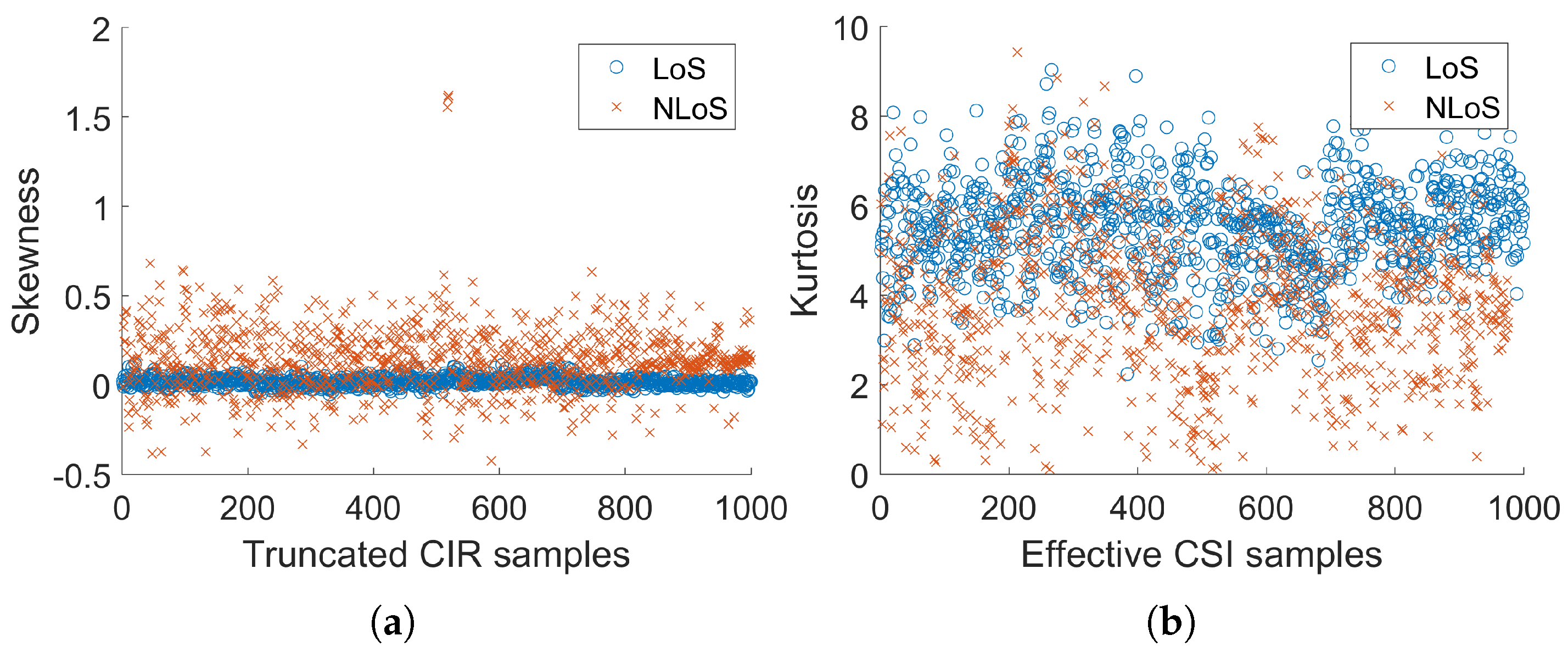
4.3. LoS Identification

Reliable lateration and angulation presupposes the presence of a dominant LoS path, whereas indoor environments, characterized by numerous obstacles, pose significant challenges, as radio waves are subject to various phenomena such as reflection, scattering, and diffraction. We propose utilizing the difference in received signal strength between dual-frequency bands to help in identifying LoS conditions. Theoretical preliminaries derive from the foundational one-slope path-loss model [31], in which the received power is given by
P r x , f = P r x 0 , f 10 η f log 10 d / d 0 ,
where P r x 0 , f is the received power at the reference distance d 0 , which can be estimated using a free space formula, or experimentally, η f is the path loss exponent which is calculated using interpolation.
In [32], a series of experiments were conducted across a broad frequency spectrum, revealing that as frequency increases, the attenuation in NLoS scenarios becomes significantly more pronounced compared to LoS conditions. The frequency dependence of the path loss exponent was found to be linked to the presence of LoS, with slight variations observed in its frequency dependence between LoS and NLoS cases. Specifically, NLoS scenarios exhibited a greater sensitivity to frequency changes as noted in [33]. Thus, we establish an indicator of NLoS severity with the discrepancy between the degree of NLoS obstruction and the attenuation differential between the two bands.
This approach necessitates acquiring the received signal strength in the satellite frequency band. However, satellite signals are typically submerged below the thermal noise floor, rendering this value—along with its inherent ambiguity—generally inaccessible directly from hardware devices. As an alternative, GNSS typically employs the Carrier-to-Noise density ratio (CN0) to quantify the quality of the received signal. The relationship between CN0 and the Signal-to-Noise Ratio (SNR) is expressed as follows: CN 0 = SNR + BW , where BW = 10 log ( b ) , with b representing the front-end bandwidth in Hz. By taking the difference between CN0 of the GNSS signals and the SNR measured in the cellular band, we effectively eliminate the noise power spectral density component, as it remains consistent across frequency bands,
SNR f 1 CN 0 , f 2 = P r x , f 1 N 0 BW f 1 + P r x , f 2 N 0 = Δ P r x 0 B W f 1 10 Δ η f log 10 ( d d 0 ) .
The resulting value represents the difference in received power, augmented by a constant offset, which can be utilized as an indicator for the proposed LoS detection method.
We further enhance the LoS indicator by analyzing the temporal and frequential characteristics of the reference signal’s CSI, which have been shown to correlate with NLoS conditions [34]. In the time domain, the focus is on the skewness of the power associated with the dominant path. This approach facilitates the truncation of the Channel Impulse Response (CIR), denoising the majority of multipath contributions by selecting only the initial samples. The skewness of truncated CIR can be calculated as follows:
s = 1 t r t = 1 t r ( | h ( t ) | | h ¯ | ) 3 1 t r t = 1 t r ( | h ( t ) | | h ¯ | ) 2 3 2 , 1 < t r < T ,
where h ( t ) = F 1 ( H ( k ) ) , F is the FFT operator, t r is the truncated parameter which is set based on the bandwidth and the typical indoor propagation delay, for instance, given 100 MHz bandwidth and typical indoor maximum excess delay of 500 ns [35], at most t r = 50 , are relevant to multipath propagation.
In the frequency domain, we focus on the kurtosis of the effective CSI, which is normalized to the same frequency in order to compensate for the effects of small-scale fading [36]. The kurtosis of the effective CSI can be calculated as follows:
κ = 1 K k = 1 K H eff k H ¯ eff 4 1 K k = 1 K H eff k H ¯ eff 2 2 , H eff ( k ) = f k f c · H ( k ) .
where f c is the central frequency and f k represents the frequency of the subcarrier k.
In general, the skewness feature under NLoS conditions exhibits a larger positive trend. In LoS-dominant scenarios, the rich superposition leads to severe frequency-selective fading; thus, the kurtosis feature is less concentrated when the NLoS path dominates.
The LoS identification problem aims to determine the presence of a direct LoS path amidst multipath propagation for each receiver location, considering all three aforementioned features. In our approach, we adopt a soft-switching mechanism that directly leverages the classifier’s output to generate a LoS confidence indicator, providing a probabilistic measure of LoS availability rather than a strict binary decision.

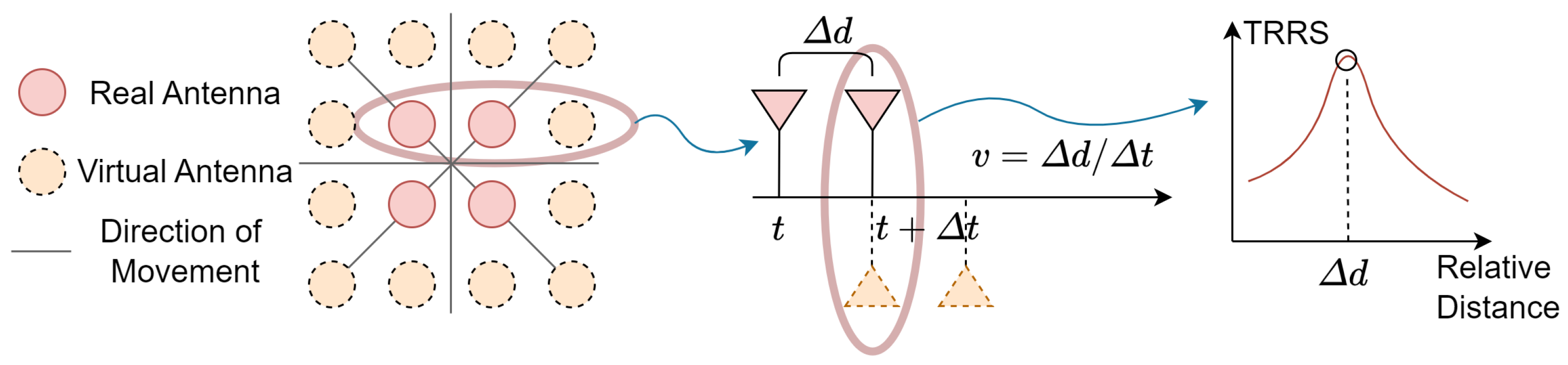
4.4. Inertial Measurements with Virtual Antenna Alignment

To enable continuous positioning in the presence of NLoS conditions, the time-reversal focusing effect is adapted to the 5G NR channel. When the calculated CIR samples are combined with their time-reversed and conjugated counterparts, they constructively interfere at the intended location while exhibiting incoherent behavior elsewhere. Consequently, the Time-Reversal Resonating Signal Strength (TRRS) is introduced as a metric to quantify the effectiveness of the time-reversal focusing effect [37], defined as
τ ( h 1 , h 2 ) = max i ( h 1 g 2 ) [ i ] 2 h 1 , h 1 g 2 , g 2 ,
where * denotes linear convolution, , is the inner product operator, and g 2 is the time-reversed and conjugated version of h 2 , i.e., g 2 [ k ] = h 2 [ T 1 k ] , k = 0 , 1 , , T 1 . Figure 3 illustrates the concept of virtual antenna alignment during motion and the corresponding TRRS value of an antenna pair.
To determine the moving speed and direction, we match the multipath profile of antenna i against those of antenna j throughout a sliding window to pinpoint the precise alignment delay. Considering a window of length 2 W , the TRRS vector is calculated as G i j ( t ) = τ h 1 ( t ) , h 2 ( t l ) , l = W , , W T , where l denotes the time lags. Thus, if the antennas move for a period of T, we obtain a TRRS matrix,
G i j = G i j t 1 G i j t 2 G i j t T .
By calculating such a TRRS matrix for every pair of antennas, the motion parameters are then estimated by identifying the aligned pairs from the TRRS matrices and continuously estimating the time delays, and accordingly the moving speed. For a given time instance, we search through the column of the TRRS matrix corresponding to that time sample to identify the maximum indicator value. The antenna pair associated with the matrix containing this maximum value reflects the movement direction, with the polarity (forward or reverse) determined by whether the maximum value resides in the upper or lower half of the matrix. The movement speed is inferred from the row index of the maximum value within the matrix, which corresponds to the window length. By identifying the time lags associated with these maximum values across the columns of the TRRS matrix, we can determine the alignment delays.
Building upon the TRRS matrix, in addition to velocity and direction estimation, we introduce two supplementary observational mechanisms: zero-velocity updates (ZUPTs) and loop closure (LC) detection.
TRRS-Based Zero-Velocity Updates: When the UE remains stationary, its signal alignment with itself remains unchanged across all antennas. Consequently, each antenna’s self-TRRS matrix G i i maintains a peak value at any time lag within the time window. This characteristic enables the precise identification of the terminal’s stationary state, providing additional observations related to position, velocity, and other system states.
TRRS-Based Loop Closure Detection: If, after a prolonged movement period, the self-TRRS matrix G i i of each antenna exhibits a significant correlation with its earlier states, it indicates that the terminal has returned to a previously visited location, forming a movement loop. Detecting such loop closures offers valuable constraints for position estimation, enhancing localization accuracy over extended trajectories.

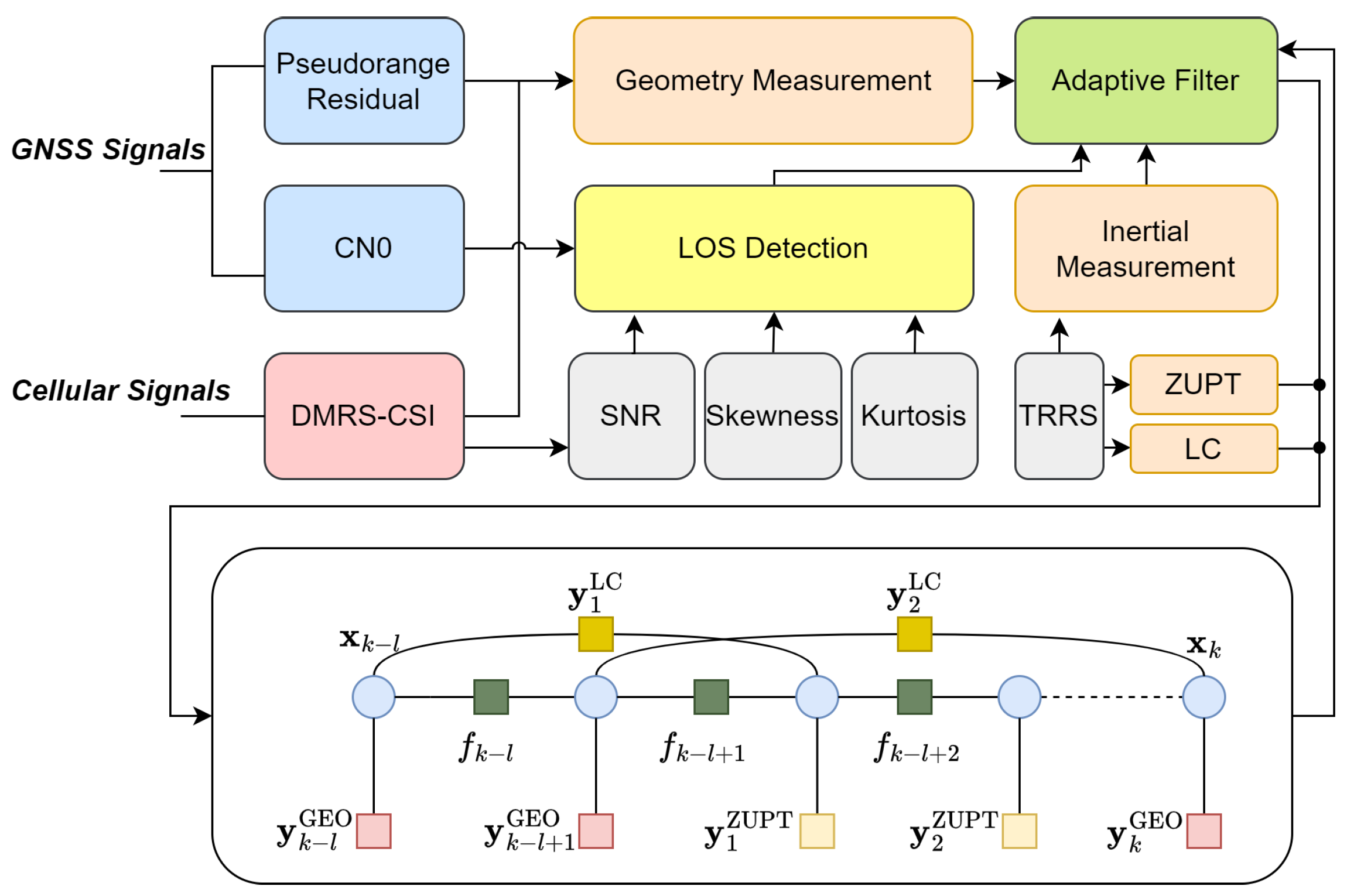
5. Localization Algorithm

In this section, we propose a Hybrid Adaptive Filter-Graph Fusion (HAF-GF) algorithm that synergistically integrates lateration and angulation estimates with inertial measurements while incorporating the predicted LoS conditions. The fusion process is carried out in two stages, an adaptive filter followed by optimizing a factor graph.

5.1. Adaptive Filter

We employ an Adaptive Extended Kalman Filter (AEKF) to enable real-time localization by dynamically adjusting noise parameters based on LoS confidence and system state variations. The AEKF framework is specifically designed to achieve weighted fusion of position estimates derived from geometric measurements and predictions obtained through radio-inertial measurements. The system state vector x k = ( x k , y k , v k , ϕ k ) at time step k is defined as a combination of position and velocity vectors, while the dynamical model follows a constant-velocity mechanization approach, wherein the position is computed as the time integral of velocity, a process widely known as dead reckoning (DR). On the other hand, the observation model incorporates position estimates deduced from geometric measurements,
x k | k 1 = f k ( x k 1 | k 1 ) + u k , u k N ( 0 , Q k ) y k = h k ( x k | k 1 ) + w k , w k N ( 0 , R k )
where y k is the geometric position measurement, u k is the Gaussian process noise, and w k is the Gaussian measurement noise. The dynamics and measurements are specified in terms of the state transition model f k and observation model h k , and the process covariance matrix Q k characterizes the uncertainty in pose increments obtained from pre-integrated velocity and heading measurements.
The key aspect of adaptive adjustment lies in the update the measurement noise based on the LoS confidence score. Notably, the relationship between the LoS confidence and measurement noise is not strictly linear. Instead, when the LoS score remains at consistently high or low levels, small variations within this range should have minimal impact on the measurement noise. To account for this nonlinearity, a sigmoid function is employed to scale the measurement noise,
R k = α c k · R 0 , α c k = α min + α max α min 1 + exp γ c k δ
where c k is the LoS confidence output by a binary classifier, α max , α min represent the scaling coefficient, defining the maximum and minimum values, which are set to 1 and 0, respectively. The parameter γ controls the steepness of the function, with a default value of 1, while δ denotes the confidence midpoint, set to 0.5.

5.2. Factor Graph

The adaptive filter provides rapid recursive state estimation, delivering real-time feedback, which is crucial for navigation and control applications. However, in complex indoor environments characterized by multipath fading, NLoS conditions, and dynamic environmental changes, geometric measurements may become unreliable. Over extended motion trajectories, particularly in highly nonlinear scenarios, accumulated errors can lead to drift and even filter divergence.
To address this challenge, we propose a batch refinement mechanism by constructing a factor graph [38] that systematically corrects AEKF estimates. The refined system state is subsequently fed back as an updated initial condition to the AEKF, thereby maintaining real-time performance while mitigating errors induced by nonlinearities. Initially, the state estimates produced by the AEKF are collected over a sliding window to form the state nodes, denoted as X k = { x k l | k l , , x k | k } . Concurrently, the available measurements—including geometric measurements derived from lateration and angulation, TRRS-ZUPT, and TRRS-LC—are incorporated as corresponding factors within the graph, denoted as Y k = Y k GEO , Y k LC , Y k ZUPT .
The DR data in one update cycle are pre-integrated at the coordinate system, the position increments are obtained through dead reckoning function f, the factor node is represented as the error function that needs to be minimized, and the DR factor node expression is as follows:
J DR X k = i = k l k x i f i x i 1 Q 1 2
where · Q 1 2 denotes the square Mahalanobis distance with covariance matrix Q .
Geometry measurements provide the position information by combining the ranging estimation from Equation (6) and angle estimation from Equation (10), and the error function is expressed as
J GEO X k = i = k l k x i y i GEO R i 1 2 , y i GEO = ( x i GEO , y i GEO ) Y k GEO
ZUPT updates provide the position and velocity information trigger by analyzing the self-TRRS matrix of each antenna, and the error function is expressed as
J ZUPT X k = i Z x i y i ZUPT Z 1 2 , y i ZUPT = ( x i 1 , y i 1 , 0 , ϕ i 1 ) Y k ZUPT
Since ZUPTs enforce velocity and heading constraints during stationary periods, it is crucial to assign high confidence weights when the device is truly motionless. Consequently, the corresponding covariance matrix Z should be set to sufficiently small values to reflect this high certainty.
Similarly, loop closure constraints can offer absolute positional information by aligning self-TRRS matrices over time. These constraints exhibit confidence levels comparable to those of ZUPT, and their associated error function can be formulated as follows:
J LC X k = i L x i y i LC L 1 2 , y i LC = ( x i LC , y i LC ) Y k LC
By exploiting Cholesky decomposition and constructing a nonlinear factor graph using a Gaussian mixture model, the factor graph optimization model is established. Consequently, the state vector estimation process is reformulated as a problem of minimizing a nonlinear function, wherein multiple cost functions are jointly optimized. This optimization problem can be tackled by performing a first-order Taylor series expansion of the cost function and subsequently solving it using the Levenberg–Marquardt algorithm [39].
The detailed workflow of the proposed localization algorithm, as illustrated in Figure 4, is outlined as follows. Initially, raw GNSS observations are collected and processed to derive pseudorange residuals and the CN0 metric. Concurrently, reference signals are extracted from the 5G PBCH channel, and channel estimation is performed to obtain the CSI matrix. This enables the computation of key characteristics, such as SNR, CSI skewness, kurtosis, and TRRS. Following this, LoS detection is conducted based on the disparity in received signal strengths across dual frequency bands and the temporal–frequential characteristics of the CSI. These observations are fused by the AEKF, and the outputs of AEKF are considered state nodes, optimized by multiple factors including ZUPT and loop closures. This two-stage estimation framework aims to enhance positioning accuracy by facilitating the rapid convergence of the factor graph while simultaneously improving the robustness of the AEKF through feedback from the factor graph.

6. Experiments and Results

The proposed scheme assumes the installation of distributed antenna systems and the use of both center frequency at 1.5 GHz (L1 frequency band of GPS) and 5.2 GHz signals in an indoor environment. For the simulation, a geometry-based channel is created by using a ray-tracing method with real spatial information. Figure 5 represents the 3D view of the test case and the ray-tracing visualizations and image of raw CSI data collected at a sample location. Our ray-tracing model follows the terms of the 3GPP specification TR 38.901 [40], setting the maximum order of reflection on a path without diffraction as 2 for reasons of simplicity and simulation speed. Only LoS and specular reflection paths are considered in this work to alleviate the computational burden. We generate 5G NR signals with 100 MHz of bandwidth resources, corresponding to 273 resource blocks and 30 kHz subcarrier spacing. The PBCH-DMRS is adopted as the pilot signal in the downlink direction, in accordance with the previous section. Finally, the received signal at the UE is used to conduct channel estimation, then the CSI matrices are stored as the raw estimation results.

6.1. Analysis of LoS Identification

According to Equation (12), the difference in SNR and CN0 between different frequency bands is highly related to the difference in received signal power. With the same transmission power, this difference corresponds to the variation in path loss. In the experiment, we set two central frequencies for the transmission segment, both with a transmission power of 0 dBm. Subsequently, at every 0.1 m interval along the vertical axes within the space, we calculate the signal reception power. Figure 6 illustrates the path loss distribution at 0.5 m height when only one specific distributed antenna is considered at the center of the building. The attenuation difference between the two frequency bands is observed to be more pronounced under challenging NLoS conditions.
The temporal–frequential CSI also indicates the LoS condition. For evaluation, we extract CSI data from 2000 locations measured under typical LoS and NLoS conditions and compute the corresponding CSI characteristics. Figure 7 presents a comparison of the CIR measurement statistics between LoS and NLoS conditions. It is obvious that the skewness of the truncated CIR and the kurtosis of the effective CSI can be utilized to differentiate between LoS and NLoS conditions. Distinct gaps are observed between the two scenarios, and in the majority of cases, LoS and NLoS conditions are linearly separable.
To evaluate the overall performance of the proposed LoS identification features, we present the Receiver Operating Characteristic (ROC) curves, which illustrate the trade-off between detection probability and false alarm probability across varying decision thresholds. A logistic regression model is constructed by integrating all three extracted features, which demonstrates significantly improved discrimination capability compared to using each feature individually. The logistic regression model and individual binary decision thresholds are trained, in which the transmitter is centrally located. For evaluation, the transmitter is repositioned to different environments—specifically, inside the conference room and at a corner of the hall—to prevent overfitting and assess the robustness of the features and detection algorithm under environmental variation.
The ROC curves corresponding to the two test scenarios are illustrated in Figure 8. The results confirm that the proposed model offers superior capability in distinguishing between LoS and NLoS conditions, even under varying transmitter placements. When constrained to a fixed false positive rate of 10%, models relying solely on either the dual-frequency received power difference or CSI kurtosis achieve detection accuracies of approximately 60% to 70%. In contrast, the combined feature model significantly outperforms individual features, attaining detection accuracies of 91.7% and 90.6% in the two respective cases.

6.2. Analysis of Inertial Measurement

We employ a rectangular antenna array to verify the feasibility of inertial observables from virtual antenna alignment, with orientation measurements constrained to the directions defined by parallel antenna pairs. This configuration inherently restricts the direction measurements to eight distinct orientations. As illustrated in Figure 9, the TRRS matrix, computed from pairwise antenna combinations, captures the trajectory of the test antenna array along a triangular path. While observation noise introduces occasional ambiguities during directional transitions, the overall capability to discriminate between different antenna pair directions is evident. Discrepancies between the true motion heading and the orientation of the antenna pair introduce additional errors in estimation. These directional mismatches can be effectively mitigated by enhancing the geometric diversity of the antenna layout, for instance, adopting a hexagonal array configuration.
Speed estimation is the core of the DR procedure, as orientation has been defined by parallel antenna pairs. To emulate natural human mobility, the receiver moved randomly at speeds below 2 m/s for a duration exceeding five minutes. Figure 10a,b present the comparison between true and estimated speeds. While errors in antenna pair discrimination occasionally lead to significant speed estimation deviations, the approach demonstrates high fidelity to the true movement speed. The error distribution of speed estimation is shown in Figure 10c,d. Notably, 90% of the estimated speeds exhibit an error margin of less than 0.14 m/s.
We further evaluate the use of the TRRS matrix for stationary state detection and loop closure identification. As illustrated in Figure 11, the visualizations of the TRRS matrix under both scenarios exhibit distinct temporal correlation patterns. When the receiver remains stationary for a sustained period, the elements within the corresponding self-TRRS matrix window exhibit consistently high temporal correlation (typically exceeding 0.8), while the TRRS values between different antenna pairs remain low (typically below 0.2), effectively indicating a stationary state. In loop closure experiments—where the UE traverses back and forth along four directions and repeatedly returns to the origin, this behavior is clearly reflected in the self-TRRS matrix, which displays prominent correlation peaks at corresponding time intervals.

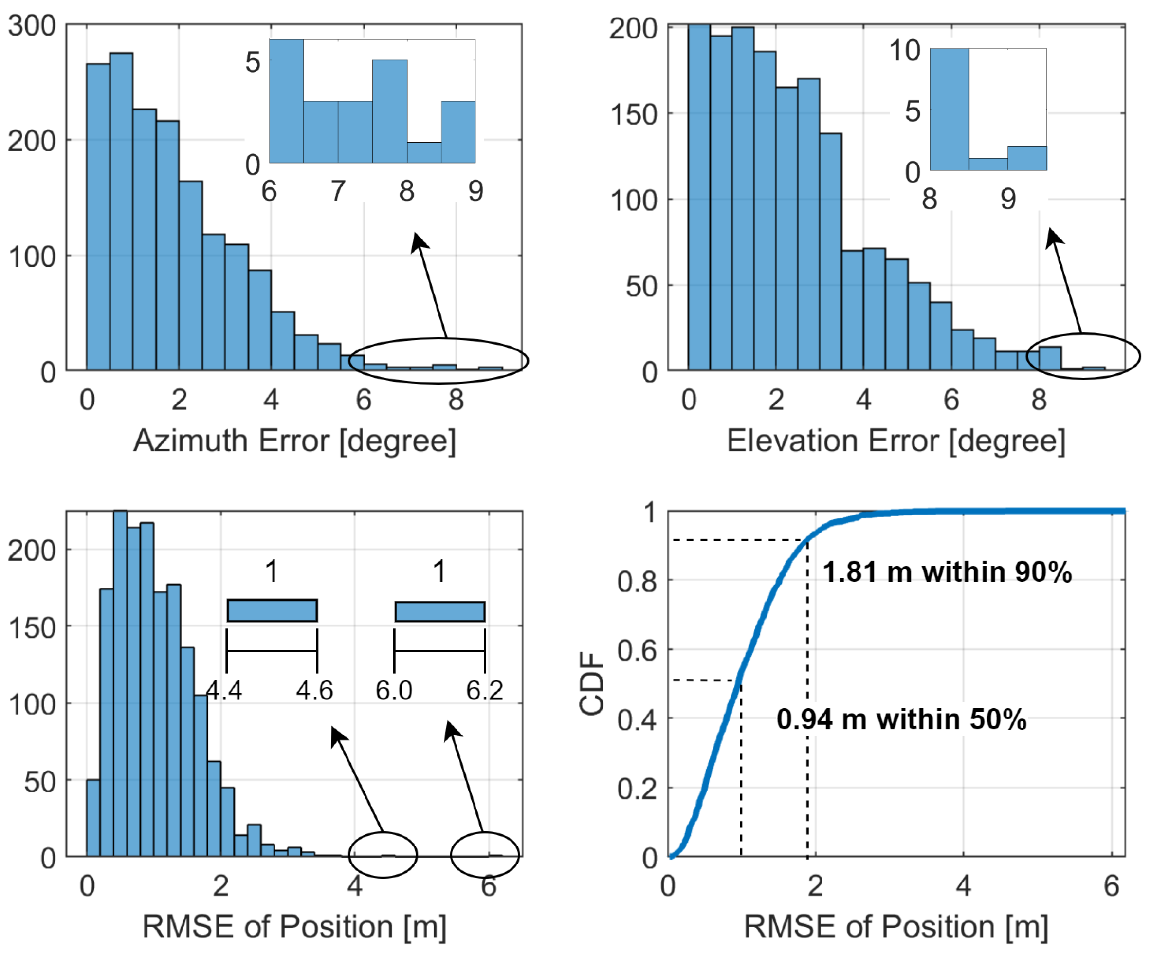
6.3. Analysis of Static Positioning

Static point positioning using the proposed method is feasible only under LoS conditions, where the accuracy depends on the precision of both distance and angular measurements. Under static conditions, the integral term in Equation (5) vanishes, leaving the range measurement error primarily influenced by pseudorange errors, characterized by the User Equivalent Range Error (UERE). UERE is defined as the square root of the sum of the squares of the individual biases, many of which can be compensated through differential correction techniques. Referring to the error budget of a practical receiver as outlined in [41], we assume a standard deviation of UERE with 1 m, accounting for factors such as receiver noise and resolution, multipath effects, and inter-channel biases.
Angular estimation errors also lead to deviations in position estimates. To assess the performance of angle estimation, we collect CSI matrices at 1800 locations under LoS conditions and perform pseudospectrum-based direction searches with an angular grid resolution of 0.5 degrees. The resulting histograms of elevation and azimuth estimation errors are illustrated in the upper part of Figure 12, revealing that even under strong LoS scenarios, the maximum angular error can reach up to about 9 degrees. By fusing range observations with directional estimates, the Root Mean Square Error (RMSE) distribution of the resulting position estimates is depicted in the lower part of Figure 12. Despite the presence of outliers caused by angular deviations, 90% of the direct localization errors remain within 1.81 m.
For further comparison with conventional positioning methods, we train a convolutional neural network (CNN) as a fingerprinting baseline using the database constructed by sampling CSI channel fingerprints at multiple known locations, following the approach in [42]. In addition, triangulation-based positioning [43] is conducted using three anchors deployed within the hall. It should be noted that both baseline methods require the ability to distinguish between different anchors for successful localization, which is only available in our GNSS-aided IBW.
The positioning error statistics are summarized in Table 1, encompassing key metrics such as Mean Absolute Error (MAE), RMSE, and Circular Error Probable (CEP) at the 75% and 90% confidence levels. As reflected in the results, all three approaches demonstrate comparable overall localization performance; however, their error distributions exhibit distinct characteristics, which are further visualized through representative positioning samples in Figure 13. The triangulation-based method is notably influenced by the spatial distribution of the UE, with accuracy degradation in regions affected by unfavorable dilution of precision (DoP). In contrast, the performance of the fingerprinting method is contingent on the quality and spatial resolution of the pre-constructed signal database. The proposed approach generally maintains robust performance but may experience significant deviations in cases where DoA estimation errors are pronounced. Nevertheless, the proposed approach achieves localization using DoA and ToA measurements from at a single anchor, significantly enhancing deployment efficiency by at least threefold. The trade-off, however, lies in its inability to benefit from additional anchors—unlike triangulation or fingerprinting approaches—and relies on the presence of a clear LoS path.

6.4. Analysis of Dynamic Positioning

To analyze the dynamic accuracy of our proposed technique, we verify the proposed HAF-GF algorithm, on the basis of a comparative analysis with traditional EKF, and the AEKF. The EKF adopts a hard-switching mechanism according to the binary classification results from the LoS detection, while the AEKF is simply the proposed HAF-GF without the further corrections and feedback from factor graph optimization. To specifically account for changes in the channel environment, we also simulate variations in the distributed antenna deployment, placing it at different locations including the center of the building, inside a single conference room, and at the corner of the hall. The fingerprint-based methods generally cannot be applied without a new site survey, and the robustness of the proposed localization can be verified in this scenario. While the dynamic positioning relies on the inertial measurements, the performance is affected by the consistency between the antenna alignment and the true motion heading. To simulate this potential error while moving, random heading bias with zero mean and 1 ° uncertainty is added to the true trajectories. Table 2 presents the parameter configurations used in our experiments. The DR noise covariance parameters are identical for all three algorithms, while the remaining two parameter sets are specific to the HAF-GF algorithm.
The test trajectories of the evaluated algorithms under all three scenarios are depicted in Figure 14. The results demonstrate that incorporating direct positioning observations significantly reduces the susceptibility of inertial tracking to large deviations from the ground truth trajectory. Although direct positioning methods based on ranging and angulation may exhibit fluctuations—particularly in environments with suboptimal transmitter deployment—the integration of inertial trajectory estimation contributes to a notable enhancement in overall accuracy compared to static positioning. Furthermore, assuming a fixed height during movement helps mitigate vertical errors.
It is also evident that the EKF based on hard switching suffers from catastrophic errors in position estimation when the LoS state is misclassified, particularly when NLoS conditions are erroneously identified as LoS. In such cases, severely biased angle measurements can critically distort the results. Conversely, when true LoS conditions are misclassified as NLoS, the trajectory can typically still be tracked based on motion prediction. Both AEKF and HAF-GF mitigate the adverse effects of geometric measurement biases through adaptive filtering. However, compared to EKF, they also introduce minor fluctuations under NLoS conditions due to noise adaptation. The HAF-GF further optimizes system states over a time window and leverages additional observations such as ZUPT and loop closures, effectively compensating for drift in dead-reckoning estimates. As a result, regardless of the anchor deployment configuration, it demonstrates the highest consistency with the ground-truth trajectory across all three evaluated cases.
From the error evolution plots over time in Figure 15, it is observed that the proposed HAF-GF achieves faster convergence during the initial phase compared to conventional filters and effectively mitigates the drift accumulated through dead reckoning. The dynamic positioning performance of all three fusion methods, along with an ablation analysis of the HAF-GF framework, is summarized in Table 3. The full HAF-GF configuration, incorporating both ZUPT and LC observations, delivers the highest localization accuracy, achieving a mean positioning error of 0.38 m, with 90% of errors falling within 0.69 m. This represents a 30% improvement over the baseline AEKF method. The ablation study results indicate that LC effectively mitigates long-term drift errors, particularly during periods where DR dominates the trajectory prediction. In contrast, the benefit of ZUPT is comparatively limited, as velocity estimates remain near zero during stationary phases even in its absence. Nevertheless, ZUPT significantly reduces computational complexity: instead of computing pairwise-TRRS matrices across antennas for velocity estimation, ZUPT relies solely on self-TRRS from individual antennas. For a 2 × 2 antenna array, incorporating ZUPT reduces TRRS computation to 1 6 during stationary intervals.

6.5. Complexity Analysis

To evaluate the computational burden of the proposed localization framework, we conduct a comparative analysis against conventional approaches. Table 4 summarizes the complexity analysis of various localization algorithms, including those enhanced with inertial fusion for dynamic positioning.
For static positioning, unlike triangulation-based algorithms that require multi-source angle estimation and repeated intersection computations, the proposed method estimates only the direction of a single signal source, followed by a two-dimensional grid search over delay and angle domains on antenna pairs. This results in a computational complexity of O ( G τ G β H 2 ) , where H denotes the number of antennas in the array, making the DoA estimation module of the proposed system at most one-third as computationally intensive as that of conventional triangulation. Anchor identification and ranging involve calculating pseudorange residuals and matching them against known cable lengths from distributed antennas, which incurs a negligible cost of O ( N ) . In contrast, the complexity of fingerprinting-based methods largely depends on the underlying model architecture. While training is computationally expensive, inference is typically more efficient, with a complexity of O ( D 2 L ) , where D represents the dimensionality of the feature vector, and L denotes the total number of layers.
For dynamic positioning, the system incorporates modules such as LoS detection, TRRS-based inertial measurement processing, and data fusion. The inertial estimation is of the complexity of O ( W K H 2 ) . The self-TRRS-based ZUPT and LC processes are subsumed within it, with reduced complexity, O ( W K H ) . While both triangulation and fingerprinting frameworks can be augmented with inertial and fusion modules, fingerprinting methods typically bypass the LoS identification stage, avoiding its associated O ( K log ( K ) ) cost from IFFT, where K is the number of subcarriers. The key computational discrepancy thus lies in the data fusion approach. Fusion techniques such as hard-switching EKF and AEKF exhibit a complexity of O ( n 2 + n 3 ) , where n is the state dimension, and the O ( n 2 ) term corresponds to Jacobian evaluation and linearization, while O ( n 3 ) accounts for matrix inversion during Kalman gain computation. Factor graph optimization further enhances accuracy by jointly optimizing a window of temporally interrelated states, with a back-end complexity O ( n 2 g 2 l ) , where g is the average number of edges per node, and l denotes the window length.
We also conduct runtime experiments to evaluate the average computational time required to solve floating-point solutions for different localization methods, both with and without TRRS-based inertial fusion, on an Intel Core i5-10210U CPU. For static positioning, the proposed method achieves an average processing time of 0.08 s per epoch. In comparison, the fingerprinting approach employing a 7-layer CNN, with convolutional layers using 3 × 3 kernels and 256 filters, requires approximately 0.125 s per inference, while the triangulation-based method, which performs multiple 2D grid searches, incurs the highest cost at 0.224 s per epoch.
When incorporating TRRS-based inertial measurements, the EKF exhibits relatively low computational overhead. The primary increase in time consumption originates from the construction of the TRRS matrix. With TRRS fusion, the average computational time per epoch for triangulation and fingerprinting methods rises to 0.292 s and 0.187 s, respectively.
In the case of HAF-GF, we adopt a sliding window of length l = 10 . The resulting average runtime reaches 0.427 s per epoch, approximately 2 to 3 times that of the EKF-based approach. At certain time steps, the computational cost of HAF-GF may exceed half a second. For latency-sensitive applications, this necessitates additional optimization strategies, such as sliding-window pruning to limit optimization to recent states and ensure bounded runtime. Alternatively, the use of advanced sparse graph representations or dedicated hardware acceleration may further enhance computational efficiency.

7. Conclusions and Future Work

In this study, we proposed a GNSS-aided indoor localization framework that repurposes existing IBW infrastructure to retransmit GNSS signals indoors. This hybrid architecture minimizes additional hardware requirements and leverages pre-installed IBW systems, significantly lowering the cost and complexity of deployment. By injecting GNSS signals through outdoor antennas and distributing them across passive dome antennas, the system facilitates simultaneous GNSS and cellular signal propagation without disrupting normal communication services.
The core methodology utilizes indoor GNSS raw measurements to perform anchor identification and precise range estimation via pseudorange residual analysis, while downlink CSI-based DoA estimation supplements directional information for localization. A LoS detection mechanism based on CSI statistical patterns and dual-signal strength disparities enhances resilience under multipath-rich and NLoS conditions. The resulting LoS confidence scores dynamically inform a HAF-GF algorithm, which combines an adaptive filter with batch-based factor graph optimization that incorporates motion constraints such as ZUPT and loop closures for robust state estimation.
Ray-tracing-based simulations in an office complex show that the system achieves static localization accuracy of 1.81 m (90th percentile) and improves to 0.69 m under dynamic movement. In contrast to conventional triangulation and fingerprinting approaches—which typically demand dense transmitter deployments and extensive calibration efforts—the proposed method significantly reduces infrastructure requirements while achieving superior positioning performance.
The current research still presents certain limitations that warrant further investigation. Future work will primarily focus on the following key directions: (1) While simulation results demonstrate the theoretical feasibility and accuracy of the proposed method, real-world deployment remains essential to fully assess challenges such as cable-induced dispersion and interference among repeated GNSS signals. A real-world trial using commercial-grade hardware is under planning to validate the system’s robustness in practical environments. (2) As the accuracy of geometry-based measurements is inherently limited by the spatial configuration of distributed antennas, the design of adaptive antenna deployment algorithms tailored to heterogeneous environments is crucial. Unlike conventional DoP-driven designs, this presents a novel class of optimization problems that account for mutual interference between nodes rather than their cooperative potential. (3) Although factor graph optimization offers improved positioning accuracy, its batch processing nature introduces significant computational overhead, posing challenges for real-time deployment on mobile or resource-constrained devices. Future work will explore low-complexity variants to support efficient localization on such platforms.

Author Contributions

Conceptualization, S.Z., X.C. and Z.L.; methodology, S.Z. and X.C.; validation, S.Z.; investigation, S.Z.; writing—original draft preparation, S.Z. and X.C.; writing—review and editing, X.C. and Z.L. All authors have read and agreed to the published version of the manuscript.

Funding

This research was funded by Beijing Natural Science Foundation (No. L222047).

Data Availability Statement

The data that support the findings of this study are available from the corresponding author upon reasonable request.

Conflicts of Interest

The authors declare no conflicts of interest.

References

  1. Farahsari, P.S.; Farahzadi, A.; Rezazadeh, J.; Bagheri, A. A survey on indoor positioning systems for IoT-based applications. IEEE Internet Things J. 2022, 9, 7680–7699. [Google Scholar] [CrossRef]
  2. Kong, X.; Wu, C.; You, Y.; Yuan, Y. Hybrid indoor positioning method of BLE and PDR based on adaptive feedback EKF with low BLE deployment density. IEEE Trans. Instrum. Meas. 2022, 72, 1–12. [Google Scholar] [CrossRef]
  3. Wang, C.; Luo, J.; Liu, X.; He, X. Secure and reliable indoor localization based on multitask collaborative learning for large-scale buildings. IEEE Internet Things J. 2021, 9, 22291–22303. [Google Scholar] [CrossRef]
  4. Santoro, L.; Nardello, M.; Brunelli, D.; Fontanelli, D. UWB-based indoor positioning system with infinite scalability. IEEE Trans. Instrum. Meas. 2023, 72, 1–11. [Google Scholar] [CrossRef]
  5. Lu, X.; Chen, L.; Shen, N.; Dai, Y.; Zhou, T.; Chen, R. Indoor Positioning with Smartphone by Using Doppler Observations From Asynchronous Pseudolite System. IEEE Internet Things J. 2024, 12, 11904–11916. [Google Scholar] [CrossRef]
  6. Li, X. A GPS-based indoor positioning system with delayed repeaters. IEEE Trans. Veh. Technol. 2018, 68, 1688–1701. [Google Scholar] [CrossRef]
  7. Madhani, P.H.; Axelrad, P.; Krumvieda, K.; Thomas, J. Application of successive interference cancellation to the GPS pseudolite near-far problem. IEEE Trans. Aerosp. Electron. Syst. 2003, 39, 481–488. [Google Scholar] [CrossRef]
  8. Adjiashvili, D.; Bosio, S.; Li, Y.; Yuan, D. Exact and approximation algorithms for optimal equipment selection in deploying in-building distributed antenna systems. IEEE Trans. Mob. Comput. 2014, 14, 702–713. [Google Scholar] [CrossRef]
  9. Moerman, A.; Van Kerrebrouck, J.; Caytan, O.; de Paula, I.L.; Bogaert, L.; Torfs, G.; Demeester, P.; Rogier, H.; Lemey, S. Beyond 5G without obstacles: MmWave-over-fiber distributed antenna systems. IEEE Commun. Mag. 2022, 60, 27–33. [Google Scholar] [CrossRef]
  10. Loyez, C.; Bocquet, M.; Lethien, C.; Rolland, N. A distributed antenna system for indoor accurate WiFi localization. IEEE Antennas Wirel. Propag. Lett. 2015, 14, 1184–1187. [Google Scholar] [CrossRef]
  11. Liu, Z.; Chen, L.; Zhou, X.; Jiao, Z.; Guo, G.; Chen, R. Machine learning for time-of-arrival estimation with 5G signals in indoor positioning. IEEE Internet Things J. 2023, 10, 9782–9795. [Google Scholar] [CrossRef]
  12. Papp, Z.; Irvine, G.; Smith, R.; Mogyorósi, F.; Revisnyei, P.; Töros, I.; Pašić, A. TDoA based indoor positioning over small cell 5G networks. In Proceedings of the NOMS 2022–2022 IEEE/IFIP Network Operations and Management Symposium, Budapest, Hungary, 25–29 April 2022; pp. 1–6. [Google Scholar]
  13. Zhou, X.; Chen, L.; Yan, J.; Chen, R. Accurate DOA estimation with adjacent angle power difference for indoor localization. IEEE Access 2020, 8, 44702–44713. [Google Scholar] [CrossRef]
  14. Stahlke, M.; Feigl, T.; García, M.H.C.; Stirling-Gallacher, R.A.; Seitz, J.; Mutschler, C. Transfer learning to adapt 5G AI-based fingerprint localization across environments. In Proceedings of the 2022 IEEE 95th Vehicular Technology Conference: (VTC2022-Spring), Helsinki, Finland, 19–22 June 2022; pp. 1–5. [Google Scholar]
  15. Wang, C.; Jin, X.; Xia, C.; Xu, C.; Sun, Y.; Duan, Y. 5G1M: Indoor Fingerprint Positioning Using a Single 5G Module. IEEE Sens. J. 2024. [Google Scholar] [CrossRef]
  16. Liu, C.; Tian, Z.; Zhou, M.; Yang, X. Gene-Sequencing-Based Indoor Localization in Distributed Antenna System. IEEE Sens. J. 2017, 17, 6019–6028. [Google Scholar] [CrossRef]
  17. Shin, B.; Lee, J.H.; Kim, C.; Jeon, S.; Lee, T. LTE RSSI Based Vehicular Localization System in Long Tunnel Environment. IEEE Trans. Ind. Inform. 2023, 19, 11102–11114. [Google Scholar] [CrossRef]
  18. Zhang, L.; Chu, X.; Zhai, M. Machine learning-based integrated wireless sensing and positioning for cellular network. IEEE Trans. Instrum. Meas. 2022, 72, 1–11. [Google Scholar] [CrossRef]
  19. Jee, G.I.; Choi, J.H.; Bu, S.C. Indoor positioning using TDOA measurements from switching GPS repeater. In Proceedings of the 17th International Technical Meeting of the Satellite Division of The Institute of Navigation (ION GNSS 2004), Long Beach, CA, USA, 21–24 September 2004; pp. 1970–1976. [Google Scholar]
  20. Im, S.H.; Jee, G.I.; Cho, Y.B. An indoor positioning system using time-delayed GPS repeater. In Proceedings of the 19th International Technical Meeting of the Satellite Division of The Institute of Navigation (ION GNSS 2006), Fort Worth, TX, USA, 26–29 September 2006; pp. 2478–2483. [Google Scholar]
  21. Vervisch-Picois, A.; Samama, N. Interference mitigation in a repeater and pseudolite indoor positioning system. IEEE J. Sel. Top. Signal Process. 2009, 3, 810–820. [Google Scholar] [CrossRef]
  22. Xu, R.; Chen, W.; Xu, Y.; Ji, S. A new indoor positioning system architecture using GPS signals. Sensors 2015, 15, 10074–10087. [Google Scholar] [CrossRef]
  23. Li, X. Gnss repeater based differential indoor positioning with multi-epoch measurements. IEEE Trans. Intell. Veh. 2021, 8, 803–813. [Google Scholar] [CrossRef]
  24. Gucciardo, M.; Tinnirello, I.; Dell’Aera, G.M.; Caretti, M. A flexible 4G/5G control platform for fingerprint-based indoor localization. In Proceedings of the IEEE INFOCOM 2019-IEEE Conference on Computer Communications Workshops (INFOCOM WKSHPS), Paris, France, 29 April–2 May 2019; pp. 744–749. [Google Scholar]
  25. Malmström, M.; Skog, I.; Razavi, S.M.; Zhao, Y.; Gunnarsson, F. 5G positioning-a machine learning approach. In Proceedings of the 2019 16th Workshop on Positioning, Navigation and Communications (WPNC), Bremen, Germany, 23–24 October 2019; pp. 1–6. [Google Scholar]
  26. Abdallah, A.A.; Jao, C.S.; Kassas, Z.M.; Shkel, A.M. A pedestrian indoor navigation system using deep-learning-aided cellular signals and ZUPT-aided foot-mounted IMUs. IEEE Sens. J. 2021, 22, 5188–5198. [Google Scholar] [CrossRef]
  27. Guo, T.; Chai, M.; Xiao, J.; Li, C. A hybrid indoor positioning algorithm for cellular and Wi-Fi networks. Arab. J. Sci. Eng. 2021, 47, 2909–2923. [Google Scholar] [CrossRef]
  28. Roy, R.; Kailath, T. ESPRIT-estimation of signal parameters via rotational invariance techniques. IEEE Trans. Acoust. Speech Signal Process. 1989, 37, 984–995. [Google Scholar] [CrossRef]
  29. 3GPP. Physical Layer Procedures for Control; Technical Report; 3rd Generation Partnership Project (3GPP): Sophia Antipolis, France, 2022. [Google Scholar]
  30. Bazzi, A.; Slock, D.T.; Meilhac, L. On spatio-frequential smoothing for joint angles and times of arrival estimation of multipaths. In Proceedings of the 2016 IEEE International Conference on Acoustics, Speech and Signal Processing (ICASSP), Shanghai, China, 20–25 March 2016; pp. 3311–3315. [Google Scholar]
  31. Retscher, G.; Tatschl, T. Indoor positioning using Wi-Fi lateration—Comparison of two common range conversion models with two novel differential approaches. In Proceedings of the 2016 Fourth International Conference on Ubiquitous Positioning, Indoor Navigation and Location Based Services (UPINLBS), Shanghai, China, 2–4 November 2016; pp. 1–10. [Google Scholar]
  32. Cepeda, R.; Thompson, W.; Beach, M.; McGeehan, J. On the measurement and simulations of the frequency dependent path loss and MB-OFDM. In Proceedings of the 2009 IEEE International Conference on Ultra-Wideband, Vancouver, BC, Canada, 9–11 September 2009; pp. 321–325. [Google Scholar]
  33. Wang, Y.; Wang, X.L.; Qin, Y.; Liu, Y.; Lu, W.j.; Zhu, H.b. An empirical path loss model in the indoor stairwell at 2.6 GHz. In Proceedings of the 2014 IEEE International Wireless Symposium (IWS 2014), Xi’an, China, 24–26 March 2014; pp. 1–4. [Google Scholar]
  34. Nkrow, R.E.; Silva, B.; Boshoff, D.; Hancke, G.; Gidlund, M.; Abu-Mahfouz, A. NLOS identification and mitigation for time-based indoor localization systems: Survey and future research directions. ACM Comput. Surv. 2024, 56, 1–41. [Google Scholar] [CrossRef]
  35. Jin, Y.; Soh, W.S.; Wong, W.C. Indoor localization with channel impulse response based fingerprint and nonparametric regression. IEEE Trans. Wirel. Commun. 2010, 9, 1120–1127. [Google Scholar] [CrossRef]
  36. Wu, K.; Xiao, J.; Yi, Y.; Chen, D.; Luo, X.; Ni, L.M. CSI-based indoor localization. IEEE Trans. Parallel Distrib. Syst. 2012, 24, 1300–1309. [Google Scholar] [CrossRef]
  37. Wu, C.; Zhang, F.; Fan, Y.; Liu, K.R. RF-based inertial measurement. In Proceedings of the ACM Special Interest Group on Data Communication, Beijing, China, 19–23 August 2019; pp. 117–129. [Google Scholar]
  38. Yang, L.; Wu, N.; Li, B.; Yuan, W.; Hanzo, L. Indoor localization based on factor graphs: A unified framework. IEEE Internet Things J. 2022, 10, 4353–4366. [Google Scholar] [CrossRef]
  39. Dellaert, F. Factor Graphs and GTSAM: A Hands-On Introduction; Georgia Institute of Technology: Atlanta, GA, USA, 2012. [Google Scholar]
  40. 3GPP. Study on Channel Model for Frequencies from 0.5 to 100 GHz; Technical Report; 3rd Generation PartnershipProject (3GPP): Sophia Antipolis, France, 2022. [Google Scholar]
  41. Medina, D.; Gibson, K.; Ziebold, R.; Closas, P. Determination of pseudorange error models and multipath characterization under signal-degraded scenarios. In Proceedings of the 31st International Technical Meeting of the Satellite Division of the Institute of Navigation, ION GNSS+ 2018, Miami, FL, USA, 24–28 September 2018. [Google Scholar]
  42. Wang, X.; Gao, L.; Mao, S.; Pandey, S. CSI-based fingerprinting for indoor localization: A deep learning approach. IEEE Trans. Veh. Technol. 2016, 66, 763–776. [Google Scholar] [CrossRef]
  43. Shao, H.J.; Zhang, X.P.; Wang, Z. Efficient closed-form algorithms for AOA based self-localization of sensor nodes using auxiliary variables. IEEE Trans. Signal Process. 2014, 62, 2580–2594. [Google Scholar] [CrossRef]
Figure 1. System model of the GNSS-aided in-building wireless. Outdoor GNSS signals are captured by a rooftop antenna and injected into the IBW via couplers. Each distributed antenna passively rebroadcasts a delayed copy of the GNSS signal alongside the cellular service signal.
Electronics 14 02079 g001
Figure 2. Procedure of 5G NR CSI acquisition through the PBCH-DMRS.
Electronics 14 02079 g002
Figure 3. An illustration of virtual antenna alignment and TRRS between two antennas. When the antenna array moves, the real antenna will be spatially aligned with a virtual antenna at a particular location. The moving speed can thus be estimated as v = Δ d / Δ t .
Electronics 14 02079 g003
Figure 4. Localization procedure of the proposed HAF-GF algorithm. In the factor graph formulation of the problem, state nodes are shown as circles, and factor nodes (measurements) are shown as squares.
Electronics 14 02079 g004
Figure 5. (a) The 3D map and ray-tracing visualizations of the test environment. (b) The estimated CSI of a sample location.
Electronics 14 02079 g005
Figure 6. Path loss map on the 0.5 m height plane for a centrally deployed distributed antenna at different frequency bands. (a) 1.5 GHz band. (b) 5.2 GHz band.
Electronics 14 02079 g006
Figure 7. (a) Truncated CIR and (b) effective CSI statistics under NLoS/LoS conditions.
Electronics 14 02079 g007
Figure 8. Overall LoS identification performance of the features and their combination where the transmitter is placed (a) in the conference room, and (b) at the corner of the hall.
Electronics 14 02079 g008
Figure 9. TRRS matrix between antenna pairs when a 2 × 2 antenna array moves in a triangular trajectory with constant velocity.
Electronics 14 02079 g009
Figure 10. Comparison of true speed and estimated speed during a trace of 5 min. (a) Speed estimation results. (b) Estimation error in m/s. (c) The histogram of speed error. (d) The cumulative error probability of absolute speed error.
Electronics 14 02079 g010
Figure 11. (a) TRRS matrix for ZUPT updates: When the UE remains stationary, the entries of the self-TRRS matrix exhibit consistently high values across all window indices. (b) Self-TRRS matrix for loop closures: When the UE revisits a previously traversed position, the corresponding entries in the self-TRRS matrix display elevated values at the relevant window indices.
Electronics 14 02079 g011
Figure 12. Histograms and cumulative distribution function (CDF) plot of the absolute angular error and static position’s RMSE.
Electronics 14 02079 g012
Figure 13. Static positioning errors of compared methods; anchors are indicated by circles with bold outlines. (a) Triangulation method. (b) Fingerprinting method. (c) Proposed method.
Electronics 14 02079 g013
Figure 14. Dynamic positioning results of compared algorithms with distributed antenna tested at varying locations: (a) Test case #1—anchor placed at center. (b) Test case #2—placed at conference room. (c) Test case #3—placed at hall corner. Color coding follows CAD standards: light blue (spatial boundaries), dark blue (internal walls), orange (furniture), green/pink (special zones).
Electronics 14 02079 g014
Figure 15. Dynamic positioning errors over time of compared algorithms. (a) Test case #1. (b) Test case #2. (c) Test case #3.
Electronics 14 02079 g015
Table 1. Static positioning performance of the compared methods.
MethodNumber ofMAERMSECEP75CEP90
Anchors(m)(m)(m)(m)
CSI-fingerprinting41.101.231.401.96
CSI-triangulation31.021.431.442.03
Proposed method11.071.581.371.81
Table 2. Covariance matrix parameter settings for the tested positioning algorithms.
ParameterDescriptionComponentsValues
Q DR process noise diag ( σ x 2 , σ y 2 ) diag ( 0.1 2 , 0.1 2 )
Z ZUPT constraint noise diag ( σ x 2 , σ y 2 , σ v 2 , σ ϕ 2 ) diag ( 0.03 2 , 0.03 2 , 0.01 2 , 0.1 ° )
L LC constraint noise diag ( σ x 2 , σ y 2 ) diag ( 0.05 2 , 0.05 2 )
Table 3. Dynamic positioning performance and ablation study results of the algorithms.
AlgorithmMAERMSECEP75CEP90
(m)(m)(m)(m)
hard-switching EKF0.931.291.572.16
soft-switching AEKF0.570.860.851.05
HAF-GF w/o ZUPT0.400.410.560.69
HAF-GF w/o LC0.450.680.670.85
HAF-GF w/o ZUPT and LC0.460.700.670.85
HAF-GF with ZUPT and LC0.380.410.550.69
Table 4. Computational complexity and time cost comparison of positioning methods.
MethodDoANetworkLoSTRRSFusionAverage Time
EstimationInferenceDetectionComputationAlgorithmCost (s)
CSI-triangulation O ( G τ G β H 2 ) 0.224
+EKF O ( G τ G β H 2 ) O ( K log K ) O ( W K H 2 ) O ( n 3 ) 0.292
CSI-fingerprinting O ( D 2 L ) 0.125
+EKF O ( D 2 L ) O ( W K H 2 ) O ( n 3 ) 0.187
Proposed Method O ( G τ G β H 2 ) 0.080
+HAF-GF O ( G τ G β H 2 ) O ( K log K ) O ( W K H 2 ) O ( n 2 g 2 l ) 0.427
Disclaimer/Publisher’s Note: The statements, opinions and data contained in all publications are solely those of the individual author(s) and contributor(s) and not of MDPI and/or the editor(s). MDPI and/or the editor(s) disclaim responsibility for any injury to people or property resulting from any ideas, methods, instructions or products referred to in the content.

