1. Introduction
Localization has always played a critical role in engineering applications, including wheeled robots, drones, autonomous vehicles, and human motion tracking. Mobile robots require localization primarily for navigation or task execution. The localization problem has been extensively researched in industrial manufacturing [
1], domestic environment [
2], hospitals [
3,
4], agriculture [
5,
6], forestry [
7], and nuclear facilities [
8]. Autonomous vehicles operate without drivers, making accurate and reliable localization a crucial task [
9,
10]. The same applies to autonomous drones [
11,
12]. Human activities, such as navigating a city or a complex building, are also supported by modern localization services [
13,
14].
Localization can be classified into two types: absolute and relative. Absolute localization, also called Global Localization (GL), refers to a global non-moving inertial frame. It can exploit landmarks, maps, beacons, radio signals, or satellite signals. Relative localization, also called position tracking or local pose tracking, estimates the relative position and orientation with respect to a previous reference point. It typically relies on inertial sensors, encoders, vision sensors, or sensor fusion combining multiple modalities [
15].
Localization systems are based on different techniques such as Received Signal Strength Indicator (RSSI), Channel State Information (CSI), Sound-acoustic, Inertial Navigation System (INS), Odometry-based System, Global Navigation Satellite System (GNSS), Light Detection and Ranging (LiDAR), Laser Imaging Detection and Ranging (LADAR), and Visual Sensors.
The aforementioned technologies have advantages and disadvantages regarding range, size, cost-effectiveness, and convenience. Furthermore, not all techniques are suitable for the same environment, as their performance depends on specific conditions and may degrade in others. For example, satellite-based localization fails in indoor environments because signals are shielded by the building structures. Moreover, indoor robot applications require precision in the order of decimeters or less [
16].
For this reason, it is important to distinguish between indoor and outdoor localization techniques, as they must be managed differently, not only based on the environment type, but also on the performance required for the task. Some techniques can be used standalone, but the results can be unsatisfactory in complex environments. This results in sensor fusion solutions that combine multiple sources of information, integrating different techniques and/or technologies to enhance performance. Furthermore, multi-sensor fusion approaches execute Bayes filter algorithms such as Kalman Filter (KF), Extended KF (EKF), and Particle Filter (PF) [
17]. Such algorithms rely on probabilistic filtering techniques, such as KF [
18] and particle filters [
19], which enable recursive state estimation under uncertainty. In parallel, neural network-based methods, such as in [
17,
20], have recently gained traction for their ability to model nonlinear dynamics and fuse multimodal sensor data in data-driven frameworks.
Localization techniques can be classified into two main categories: infrastructure-free and infrastructure-based. The former exploits the existing infrastructures, such as Wi-Fi, Frequency Modulation (FM), Global System for Mobile Communication (GSM), and sound signals. The latter requires dedicated electromagnetic sources, such as Radio Frequency Identification (RFID), infrared (IR), Bluetooth, visible lights, or dedicated ultrasound sources [
21].
In the literature, many works have been proposed as review localization papers; however, they do not offer a comprehensive overview of the proposed technologies or algorithms; for example, references [
22,
23] do not consider or investigate deeply relative localization solutions (based on odometer or basic sensors such as accelerometer, gyroscope, and magnetometer), reference [
24] is focused only on indoor environments, and reference [
25] considers only robot localization.
Unlike previous works in the literature, this paper aims to provide a thorough review of the main localization technologies and algorithms for both indoor and outdoor applications. It classifies the most widely adopted approaches, explains their underlying principles, and compares their accuracy and performance. Furthermore, the main adopted algorithm for localization purposes, such as KF and PF, are emphasized. Additionally, the paper includes summary tables highlighting the key characteristics of current state-of-the-art techniques.
The rest of the paper is organized as follows. In
Section 2, the main sensors and techniques used in the field of localization are presented;
Section 3 presents the algorithms for position estimation and the main algorithms adopted in fusion-based systems, including Neural Networks (NN), which are used for different purposes;
Section 4 reports the summary tables, which include the obtained accuracies of the investigated technologies and their environmental application;
Section 5, which reports the conclusions.
2. Technologies
This section aims to provide a state-of-the-art overview of localization techniques and sensors for indoor and outdoor systems. For each technique, the applications, main idea, model, and/or approach are described, along with highlighting current research progress, typical challenges, and available solutions.
The taxonomy of localization technologies discussed in this review is summarized in
Figure 1.
2.1. Odometry
Odometry is the use of motion sensors such as encoders or optical flows to determine the robot or vehicle’s change in position relative to some previously known position. Despite its simplicity and independence from external references, it is prone to cumulative errors, which recent research seeks to mitigate through sensor fusion and adaptive filtering.
2.1.1. Encoder
The encoder is an often-used technology in industrial automation, because it can determine the exact position, speed, and distance travelled by a wheeled or legged robot. However, it has a limitation due to the cumulative measurement error caused by factors such as inaccurate wheel diameter measurements, variations in wheel sizes, and counting errors in systems using drive shaft encoders, and so on. Due to integration, this error increases over time. Several studies propose combining encoder data with absolute measurements (e.g., GPS, IMU) to correct drift and improve long-term accuracy [
26]. Consequently, encoder data is primarily used to estimate relative position. In mobile robotics, encoders are essential for odometry calculations, enabling robots to navigate predefined paths with high accuracy. However, to prevent excessive error buildup, encoder data is typically fused with other sensors or systems that periodically provide an absolute position reference.
The model that represents the position of a two-wheeled mobile robot is given as [
25]:
where
is the estimated position;
and
are the coordinates of the previous position;
is the orientation;
and
the distances travelled by the right and left wheel, respectively; and
is the distance between the wheels.
2.1.2. Optical Flow
Optical flow odometry is a technique used to estimate the relative 2D translation (relative localization) of an object such as a robot or PC mouse. It exploits a miniaturized camera that captures consecutive images which are reflected from an irregular surface that is illuminated by an LED. These images are processed by comparing consecutive frames through autocorrelation to estimate the direction and magnitude of movement. This technique is especially useful in GPS-denied environments, and recent developments explore the use of multiple sensors to increase robustness. To determine both the relative position and orientation of the object, two optical flow sensors are needed. To reduce errors, it is possible to adopt an array of optical flow sensors and average the output information as proposed in [
27], where the authors proposed a system with eight optical flow sensors. This reflects ongoing efforts to develop low-cost and accurate odometry solutions for indoor localization.
The final model for a system composed of two optical flow odometry sensors, installed at distance D from each other, is given as [
28]:
where
and
are the absolute positions at the time
,
and
are the previous absolute positions at the time
,
and
are the orientations at the times
and
, and
,
, and
are the variations of
,
and
, respectively.
2.2. Radio Signal-Based Localization Techniques
Radio signal-based localization methods estimate position and orientation by extracting information from signals received from specific sources. Recent advancements in this domain target improving robustness in complex environments and reducing sensitivity to interference and multipath. This information can be derived from signal characteristics such as power, channel model, Time of Arrival (TOA), or Angle of Arrival (AOA) of the signal. Moreover, radio sources can exploit either existing infrastructure or dedicated hardware, including networks such as Ultra-Wide Band (UWB), ZigBee, Wi-Fi, cellular networks, and satellite systems. Among these, UWB is considered the best technology for precise indoor positioning systems [
29] thanks to its high time resolution and low interference, although its adoption may be limited by hardware cost and deployment complexity.
Radio signal-based localization techniques typically rely on either geometric mapping or the fingerprinting approach [
30]. These two methods improve the robustness in dynamically changing environments and are very popular in literature. Their principles and algorithms are discussed in
Section 3.1.
2.2.1. RSSI-Based Localization
RSSI is one of the earliest indicators used and is suitable for both indoor and outdoor GL systems. Some of its main applications include indoor localization, asset tracking, or Internet of Things (IoT)-based location services. The RSSI exploits the attenuation of radio signals during propagation. Essentially, it is a measurement of how well a device can receive a signal from a source. The MAC layer of widely used network technologies, such as UWB, ZigBee, Wi-Fi, and cellular networks, provides access to signal power measurements, which can be leveraged for localization. Furthermore, to determine the position of a target, RSSI-based techniques typically require at least three radio frequency sources with known positions, known as anchors [
31]. By exploiting the Log-normal Distance Path Loss (LDPL), the distance between each anchor and the target is extracted and then the position is obtained by trilateration [
30]. The LDPL model is given as:
where
is the path loss (reduction of the power) in decibels,
is the length of the path,
is the average path loss at the reference distance
, and
is the path loss exponent.
The LDPL is the most widely used model in RSSI-based localization. The accuracy of these techniques depends on the path loss exponent, which is not always well known [
30]. To estimate this parameter as accurately as possible, algorithms such as Maximum Likelihood Estimation (MLE) or Linear Least Square (LLS) are commonly used. However, a major drawback is that these methods introduce a set of nonlinear equations that are challenging to solve.
In general, on a large scale, the received signal attenuates monotonically from the transmitter to the receiver due to the dissipative nature of the channel. However, on a small scale, two phenomena affect the signal: shadowing caused by objects and obstacles in the environment, and multipath propagation [
32]. The combined effects of these phenomena give rise to a non-monotonic trend of propagation. Both geometric and fingerprinting methods are affected by small-scale signal variations, significantly impacting accuracy and matching. Recent efforts focus on developing adaptive algorithms and hybrid models to compensate for these variations in real time. Additionally, noise and interference may arise due to human activity and/or moving objects within the localization area.
RSSI-based localization can achieve submeter-level accuracy in simple indoor environments. However, this performance degrades significantly in complex environments due to multipath fading and temporal dynamics [
33]. These limitations are particularly relevant in low-power wide-area network (LPWAN) technologies such as the Long-Range Wide Area Network (LoRaWAN). In systems like these, the accuracy of pinpointing locations is low, because the RSSI-based localization is strongly affected by dynamic propagation conditions and environmental attenuation [
34]. On top of that, the TDoA-based methods require precise time synchronization between gateways and are highly sensitive to multipath effects, especially in urban or indoor environments [
35].
The primary challenges of this technique stem from its susceptibility to temporal fluctuations, which make the measurements both inconsistent and coarse-grained in complex settings [
36]. To address these challenges, the authors of reference [
37] proposed advanced machine learning techniques for enhancing RSSI-based fingerprinting; they introduced a Bag-of-Features (BoF) framework combined with a k-nearest neighbor (k-nn) classifier to improve localization accuracy in complex indoor environments. Their approach transforms raw RSS data into robust high-dimensional features using k-means clustering, mitigating the impact of multipath and signal variability. Experimental results demonstrate superior performance compared to traditional fingerprinting methods, achieving near-meter accuracy in real-world scenarios. This highlights the potential of machine learning to overcome inherent limitations of RSSI-based systems. Furthermore, an indoor environment that is rich in multipath leads to worsening wireless propagation and gives rise to unreliable results. Nevertheless, improvements can be achieved through better characterization of the propagation channel and realizing multipath effects models at a smaller scale [
38].
Alternatively, better results can be obtained by employing the Channel Impulse Response (CIR) in the time domain. The model is given as:
where
is the amplitude,
is the phase, and
is the delay of the i-th path. This model considers the channel as a temporal linear filter and allows a complete characterization of each single path of the multipath channel [
39]. Moreover, from CIR, it is possible to obtain the Channel Frequency Response (CFR) by Fourier transformation.
In a multipath channel, the signal arrives at a receiver travelling along different paths and each of them introduces a different delay. This brings a frequency diversity in the time domain where different copies of the signal are available, each one with a different phase and amplitude. The Line-Of-Sight (LOS) component can first be identified by extracting the CFR and obtaining the CIR through inverse transformation, followed by eliminating the Non-Line-Of-Sight (NLOS) path components [
39].
Considering the geometric mapping, better results can be obtained using the Multipath Distinguishing (MuD) system, proposed in reference [
40]. The technique exploits the frequency diversities in Orthogonal Frequency Division Multiplexing (OFDM) systems due to multipath channels associated with subcarriers in the sent signal. Each subcarrier is orthogonal to others and each of them can be associated with a CFR or a CIR. This enables us to find as many frequency diversities as the number of subcarriers used and to find for each of them the LOS eliminating NLOS after applying a threshold. The set of the nonlinear equations in the MuD is as follows:
where
is the received power,
denotes the reflection,
is the propagation distance,
is the wavelength, and
, where
denotes the transmitted power,
indicates the transmitter antenna gain, and
is the receiver antenna gain.
As for fingerprint mapping, RSSI cannot be used to distinguish between spatial variations from temporal variations. To overcome this issue, authors in references [
41,
42] used the channel response and normalized the amplitudes and phases extracted from the CIR to evaluate the self-correlation of the channel response at a specific location. The method considers that the correlations of the channel response in a location at different times are stronger than correlations in different locations. Considering the i-th transmitter and the j-th receiver, the formula for the distance between the new N-th measurement
and the history of measurements
is given as:
where
is the measurement history of the temporal link signatures,
is a previous measurement of temporal link signature, and
is the historical average difference between each pair of the N-1 measurements. A location change is decided if the obtained
is greater than a preset threshold.
Reference [
43] proposes a similar CIR-based technique for fingerprinting named Wide Band Neural Network-Locate (WBNN-Locate) for geolocation applications in mines. The method executed area sweeping in a certain number of locations based on channel sounders. At each location, the CIRs are extracted and from each CIR seven predetermined parameters are extracted: the mean excess delay, the Root Mean Square (RMS) delay spread, the maximum excess delay, the total received power, the number of multipath components, the power of the first path, and the arrival time (delay) of the first path. Once a receiver has measured these parameters, the localization is obtained using ANN.
The Precise indoor Localization (PinLoc) technique [
44] directly uses CFRs without inverse transformation to CIRs. It extracts the physical layer information from Wi-Fi systems, including the mean and the variance of phase and magnitude of each subcarrier. These quantities vary over time and environmental mobility, but their means and variances extracted for each training location can be used as fingerprints. Such statistical fingerprints offer improved resilience against environmental changes when compared to raw signal power values. Additionally, these features are modelled using a Gaussian distribution for each subcarrier and training location. Localization is performed by evaluating the probability of belonging to a specific position using the following expression:
where
identifies the location,
identifies the subcarrier,
is the total number of subcarriers,
denotes the variance of the f-th subcarrier at i-th location in the fingerprint database,
is the mean of the f-th subcarrier at i-th location in the fingerprint database, and
is the mean of f-th subcarrier in a generic position. The terms
and
are the vectors that include all subcarriers associated with
and
. The main issues related to channel response are bandwidth limitations and feature selections [
36]. Ongoing research aims to automate feature selection and optimize bandwidth usage to balance resolution and computational efficiency. On the one hand, the bandwidth limitation restricts the ability to extract multipath components with sharp, well-defined peaks, instead resulting in smoother signal representations. Consequently, the LOS may not be distinctly identifiable. On the other hand, the feature selection is fundamental for choosing the most location-dependent features of the channel response [
36]. Additionally, signature data from CIRs and CFRs become impractical in large areas due to computational complexity and calibration issues. Further challenges may arise in the presence of irrelevant phase shift locations [
42,
44].
2.2.2. CSI-Based Localization
RSSI-based techniques have limitations due to environmental variations caused by non-static objects and human presence. This leads to the instability of RSSI techniques that gives rise to spurious localization [
45]. In contrast, CSI addresses these challenges by providing insights into how a signal propagates from transmitters to receivers, revealing effects such as scattering, fading, power decay, and their combinations [
38].
CSI is often used in systems to detect the presence of moving objects. Applied in OFDM systems, this technique derives both the amplitude and phase of each subcarrier from CFRs and these couple of variables constitute the CSI associated with each frequency [
36]. Considering a narrowband flat-fading channel, the model of an OFDM system in the domain of frequency is given as [
38]:
where
is the received vector signal,
is the transmitted vector signal,
is the channel matrix, and
is the additive white Gaussian noise vector. From Equation (8), it is possible to estimate the CSI of all subcarriers by applying the following equation:
The CSI of each subcarrier can be represented as:
where
is the amplitude and
is the phase of each subcarrier.
The CSI techniques are applied in both fingerprint and geometric mapping methods. For example, in reference [
46], authors propose an indoor device-free motion detection system adopting a fingerprinting approach. This system, called Fine-grained Indoor Motion Detection (FIMD), requires dedicated hardware. In this work, the CSIs are expressed and collected in a vector as:
where the
is the i-th CSI that is defined by Equation (10). Defining the CSIs in a sliding temporal window as:
it is possible to obtain a matrix where each column is associated with the correlation ratio of the i-th measurement and the (i + 1)-th measurement, as follows:
where n is the total number of the settled measurements. In static environments, correlations are higher, whereas in dynamic environments with moving objects, correlations are weaker. The feature proposed by the authors of reference [
46] is:
In static environments, the correlations between each column are high, whereas in the case of dynamic environments, the correlations are low and the eigenvalues of the matrix decrease significantly.
On the contrary, authors in reference [
38] adopt the CSI with a geometric mapping approach and exploit the frequency diversities in the OFDM system, which arises from multipath channels associated with subcarriers in the transmitted signal. The proposed system, called Fine-grained Indoor Localization Algorithm (FILA), extracts the signal power corresponding to the LOS path from the CIR using a threshold-based method. The model used to find the distance is as follows:
where
is the velocity of the transmitted wave;
is the central frequency;
is the attenuation factor;
is a coefficient that includes the transmitted power, antenna gains, and all hardware factors; and
denotes the weighted sum of frequency. Moreover,
is given as:
where
is the total number of subcarriers,
is the frequency of the k-th subcarrier,
is the central frequency, and
is the amplitude of the filtered CSI.
2.2.3. Time-Based Localization
Localization based on time is used both in indoor and outdoor applications, and it exploits the TOA technique. Recent research has focused on enhancing time synchronization accuracy and mitigating NLOS errors, which are major challenges for TOA-based systems. In this approach, the radio source transmits a signal that includes a timestamp, allowing the receiver to determine the time taken for the signal to arrive. By knowing the propagation velocity, the distance between the transmitter and the receiver can be calculated. Besides the TOA technique, the TDOA method is also widely used. It determines the distance by calculating the difference between two TOAs. The time of the arrived signals and the speed of propagation are the required information for distance calculation.
To implement a TOA-based localization system, at least three APs or anchors with known locations are required to emit a synchronous signal [
31]. Generally, the positions of the anchors are fixed, but authors in reference [
47] propose a system with movable UWB anchors to control the outdoor swarm flight of Unmanned Aerial Vehicles (UAVs). This highlights ongoing efforts to improve the flexibility and adaptability of TOA-based localization in dynamic environments. The proposed system exploits the TOA and can change, in real time, the UWB anchor position. Moreover, a key advantage is that the single ground control station can dynamically modify the UWB coverage range, also in real time.
TOA-based localization performs best under LOS conditions, and, in general, the accuracy improves with increasing signal bandwidth [
36].
The GNSS operates based on the TOA principle. It is a technology that exploits an artificial satellite constellation that provides positioning, navigation, and timing services on a global or regional basis [
48]. To determine a position on or near the Earth’s surface, a GNSS receiver performs trilateration using timing signals from at least four GNSS satellites. These signals are used to extract TOA or TDOA, enabling the calculation of distances between the receiver and each satellite. The signal frequencies are in two bands: the first one is between 1.164 and 1.300 MHz, while the second one is between 1.559 to 1.610 MHz [
23].
There are different types of GNSS, namely, the Global Positioning System (GPS), which is owned by the United States, the Global Navigation Satellite System (GLONASS), which is supported by Russia, the BeiDou system, which is operated by China, and the Galileo, which belongs to the European Union [
23].
GNSS is a suitable system for outdoor applications. However, in indoor environments, the signal is attenuated significantly and/or shielded by building structures, and, consequently, it cannot be used. Furthermore, shadowing and multipath effects can occur in environments such as mountain-surrounded areas, tunnels, urban canyons (high-rise building clusters), and dense forests. To mitigate these issues, pseudolites can be used, or GNSS data can be fused with other localization technologies such as Inertial Measurement Units (IMUs) [
26], visual odometry systems [
7], or 5G, such as in the GNSS/5G Integrated Positioning Methodology [
49]. Recent studies have also proposed the integration of GNSS with odometry and low-power LPWAN technologies such as LoRaWAN to increase robustness in scenarios where satellite visibility is limited or inconsistent. Such sensor fusion approaches aim to ensure more reliable localization by combining the complementary strengths of each technology during signal degradation or temporary loss [
34].
Standalone GNSS accuracy depends on convergence time; for example, a standalone GPS solution can achieve a 10 cm accuracy after about 30 min, an accuracy less than 5 cm after about 2 h, and a millimeter accuracy after several hours [
50]. Other GNSS systems provide similar, though slightly lower, performance. Furthermore, the accuracy can be improved either by increasing the number of satellites per system or by combining more GNSS systems at the same time. The best performances are achieved when all four GNSS (GPS, BeiDou, GLONASS, and Galileo) are fused, for Precise Point Positioning (PPP). In such a case, the achieved accuracy is 10 cm after several minutes and less than 5 cm after less than 30 min of convergence [
50]. GNSS-based localization applications include autonomous vehicles (e.g., cars, trucks, ships and aircraft), robots in agriculture, and human or animal tracking [
23].
In indoor environments, TOA is based on CIR, and the corresponding time estimation techniques can be classified into two types: (i) methods that evaluate the delay associated with the LOS path from CIR; (ii) methods that execute filters based on cross-correlation evaluations [
36]. To obtain accurate time estimation, the latter requires super-resolution techniques such as the Root MUltiple SIgnal Classification (Root-MUSIC) algorithm [
51] or the Total Least Squares version of the Estimation of Signal Parameters via Rotational Invariance Technique (TLS-ESPRIT) [
36]. Initially, they were applied only to the frequency domain, but later these techniques were applied also for time domain analysis due to a strong resemblance between the CIR Equation (4) and the CFR equation expressed as:
The MUSIC algorithm, for example, estimates the pseudospectrum, which is composed of both signal subspace and noise subspace. By maximizing the MUSIC pseudospectrum, it is possible to obtain the multipath delays, as the optimal solutions in the noise subspace have zero projection [
52].
Other techniques adopt statistical approaches to find the NLOS in the signal. Such statistical methods are increasingly favored for real-time NLOS detection in dynamic indoor scenarios. These methods leverage the variance associated with LOS and NLOS conditions, as the variance tends to be significantly larger in the presence of NLOS [
53].
Besides the traditional TOA and TDOA approaches, some proposals exploit the data-acknowledgement (ACK) round to estimate the time of MAC idle and derive the distance as reported in reference [
54]. This technique, known as CAESAR, i.e., CArriEr Sense-bAsed Ranging, utilizes both the Time of Flight (ToF) of a valid data ACK and the Signal-to-Noise Ratio (SNR) measurements to obtain the distance between two stations. By using SNR measurements, the dispersion generated by the ACK detection time is evaluated to improve the accuracy in the case of multipath environments.
2.2.4. Angle-Based Localization
AOA information from radio signal can also be utilized for localization. These measurements require either more expensive antennas arranged in an array configuration or the use of a rotating directional antenna. This enables the simultaneous estimation of both distance and angle [
55]. Contrary to RSSI-based and time-based techniques, standalone AOA requires at least two anchors, each with multiple antennas, to estimate localization through angulation. However, this technique provides low accuracy when detecting distant objects [
31]. Recent studies aim to mitigate this limitation by refining antenna array calibration and applying adaptive beamforming methods.
The rotating directional antenna method measures the angle associated with the maximum strength of the signal. However, this approach may give false results, as the strongest signal direction does not always align with the actual source direction due to environmental interferences from objects or human presence [
56].
The antenna array method, on the other hand, leverages Multiple-Input Multiple-Output (MIMO) systems, which are integrated into modern wireless protocols. This technique is based on finding the CIRs associated with each antenna, which allows for the estimation of time delays. Using algorithms such as the Maximum Likelihood estimator or a simplified version like the Space-Alternating Generalized Expectation-Maximization (SAGE), the Angle of Arrival (AOA) is estimated [
56]. In addition, the estimation of the AOA
is obtained by minimizing the following equation:
where m is the m-th linearly spaced antennas at half the carrier wavelength, M is the total number of antennas,
is the CIR obtained from the m-th antenna,
is the CIR of the first arrived component, and
is the delay of the signal. The CIR can be investigated with a super-resolution algorithm, as proposed in references [
57,
58], where the authors use the MUSIC algorithm to derive AOA, adopting a configuration with two Access Points (APs) equipped with four antennas, and a receiver with two antennas.
The main drawbacks in AOA estimation stem from the use of directional antennas, which require dedicated hardware, potentially complicating the system setup. Nonetheless, AOA can be combined with other ranging techniques, as direction and distance are orthogonal variables [
36]. A hybrid approach integrating multiple techniques is proposed in reference [
59], where a Taylor series least squares method is applied to a system combining GNSS, 5G TOA, and 5G AOA. Simulation results show that this method effectively mitigates synchronization issues. In other hybrid solutions, such as AOA+RSSI in [
60] or AOA + TOA in [
61], systems are proposed that reduce the hardware requirements while improving localization accuracy.
2.3. RFID Techniques
RFID techniques provide a GL, and they are based on High-Frequency (HF) or Ultra-High-Frequency (UHF) systems. Low-Frequency (LF) RFIDs are unsuitable for localization due to their requirement for near-direct physical contact with the reader. Meanwhile, Super-High-Frequency (SHF) RFID systems exist but lack off-the-shelf hardware [
62].
RFID technology is suitable for localization in different environments, such as industries or hospitals, and applications, such as human motion tracking [
63]. They are characterized by a wide range of available tags (including passive and active types), the contactless feature, identification through a unique ID, a small size, and cost-effectiveness [
62].
2.3.1. RFID Localization Principle
RFID-based localization techniques can be classified into moving-reader-based [
64,
65] systems or moving-tag-based systems [
66,
67]. In the former, the tags are fixed in determined positions and the mobility of readers in the area is exploited. In the latter, the readers are fixed, and the tag moves freely in the workspace. As a result, knowing the positions of the tags (first case) or the readers (second case) enables the obtainment of position measurements.
HF systems rely on inductive coupling, meaning that tags do not require an external power supply. These systems detect the Electronic Product Code (EPC) of a tag within a small localization range (a few centimeters). The technique is based on the reading or not reading of the tags, which usually form a reference square or rectangular grid. Then, positioning is obtained by associating the position with the detected tag in the grid. The accuracy depends on the density of this reference setup [
64].
UHF systems exploit the modulated backscattering principle of electromagnetic waves. In this case, too, the tags do not require a power supply, since they absorb energy from the sent electromagnetic wave. Power supply-free solutions are considered passive, whereas solutions where tags are supplied and broadcast their signal continuously are considered active. An example of active solutions are the LANDMARC [
68] and the SpotON [
69] systems. Additionally, solutions that use batteries only to supply other sensors are considered semi-passive systems [
62].
Generally, the passive UHF RFID techniques can be classified into three types. In the first type, the reader transmits electromagnetic waves, which are modulated by the tag and then scattered back to the reader. Through this modulation, the tag encodes and transmits its EPC within the scattered signal. This case differs from the HF RFID solution, since the signal is scattered back by multiple tags. Consequently, a probabilistic model is required to infer the tag detection [
70].
The second type of UHF RFID technique involves extracting the RSSI from the backscattered signal measured by readers, and the ranging information is usually extracted by adopting dedicated hardware. Several internal factors, such as the tag model, chip sensitivity, orientation, antenna type, and materials used, affect RSSI measurements. Additionally, external factors, including multipath propagation, interference, and shadow zones, further complicate the RSSI model. These complexities make it challenging to develop a reliable RSSI-based localization model [
71].
The third type of UHF RFID principle adopts the phase-based localization technique, where the phase of the backscattered signal is extracted. This approach generally achieves higher accuracy than RSSI-based methods. However, it requires the correct handling of the
phase ambiguity problem, which is typically solved using phase unwrapping techniques or phasor sequence assembling [
72]. Additionally, the phase offset introduces another issue, which can be solved with the Phase Difference of Arrival (PDOA) technique [
73]. TOA or TDOA-based approaches are not suitable for RFID techniques, due to the limited available bandwidth [
74].
Passive RFID systems are highly sensitive to environmental conditions, particularly in the presence of metals or liquids, which can reflect or absorb radio waves, leading to degraded signal quality and localization performance [
75]. This is especially problematic in UHF systems where electromagnetic propagation is more susceptible to interference. To mitigate these limitations, strategies include using on-metal RFID tags designed with shielding or optimized antenna configurations [
76], frequency diversity, or incorporating RFID into hybrid systems that leverage complementary technologies such as UWB or vision systems to enhance reliability and robustness in challenging environments [
62,
66].
In general, the achievable accuracy of RFID-based localization systems varies with factors such as frequency band, tag type (active, passive, or semi-passive), environment, and the localization technique employed (e.g., RSSI, phase-based, or grid-based methods). Passive HF systems, when deployed with dense tag grids in controlled environments, can attain centimeter-level accuracy (5–10 cm) [
64,
77,
78]. Passive UHF systems utilizing RSSI measurements have demonstrated localization errors as low as 5.7 cm in unidimensional setups [
79,
80].
Phase-based localization techniques, leveraging phase difference measurements between antennas, have achieved millimeter-level accuracy under ideal conditions [
81]. Active RFID systems, such as those based on LANDMARC, typically provide 1–2 m accuracy [
68], while hybrid systems can reduce this to the sub-meter range [
82,
83]. However, accuracy drops significantly in environments with high interference or limited tag density.
Some particularly interesting works in the literature are as follows. Authors in reference [
84] propose a robot tracking system that uses a passive RFID solution and exploits a B-spline Surface algorithm to solve the tracking location equations instead of using the Look-up Tables approach. Reference [
65] proposes a system that uses Angle Compensation and KF. In this approach, the RSSIs of the backscatter signal from the nearby RFID tags are measured. In the first step, the algorithm estimates the location of the readers by using a database and neglecting the tag–reader angle-path losses. In the second step, by exploiting the previously estimated location and using trilateration or any other appropriate algorithm, an iterative procedure refines the tag–reader angle-path losses estimation to improve reader position accuracy. In reference [
85], the authors propose a system that uses an EKF and the Rauch-Tung-Striebel (RTS) smoother to solve the wavelength ambiguity of phase measurements. The system state consists of the position, velocity, and phase offsets of the antennas.
2.3.2. Sensor-Fusion with RFID Techniques
The greater the number of tags (or readers, in the case that the tag is in motion), the higher the accuracy of localization. However, this technology must be matched with accuracy and economic constraints. RFID techniques can be used as standalone solutions or integrated into a sensor-fusion framework (giving rise to hybrid RFID-based localization systems). In the latter case, incorporating additional techniques and sensors helps reduce tag density while improving localization performance [
62,
74,
86]. For instance, in reference [
87], a hybrid system that combines Wireless Sensor Networks (WSNs) and RFID technologies to enhance indoor positioning accuracy is presented. The integration leverages the strengths of both systems, with WSNs providing continuous monitoring and RFID offering precise identification. Authors in reference [
88] propose a system that fuses RFID and WLAN to support both accurate indoor positioning and mobility management; the RFID system exploits an anti-collision algorithm named Pure and Slotted Aloha. Authors of reference [
89] demonstrate how combining WLAN fingerprinting and RFID can overcome the limitations of each technique when used independently. Similarly, reference [
90] presents a hybrid RFID-WLAN solution employing textile RFID tags to localize individuals in indoor spaces with improved flexibility. These hybrid approaches address challenges such as multipath interference, shadowing, and limited read range, ultimately leading to more reliable and scalable localization frameworks.
Reference [
62] classifies the localization techniques into three cases: (i) standalone systems that rely only on RFID; (ii) fused systems that merge RFID and proprioceptive sensors; and (iii) fused systems that integrate RFID and exteroceptive sensors. Additionally, proprioceptive and exteroceptive sensors can be used together, forming a fourth category known as a hybrid system.
Proprioceptive approaches often employ IMU [
67] or odometry measurements [
91], typically executed in two steps. First, the proprioceptive data are used to estimate the prior probability distribution of the localization. Then, RFID data are incorporated for correction, refining the posterior probability distribution. These distributions are continuously and recursively calculated in localization algorithms.
In the exteroceptive case, RFID systems are often fused with camera vision systems [
66], Laser Range Finder (LRF) [
92], RF systems (Bluetooth, Wi-Fi, ZigBee, and so on) [
93], and acoustic systems [
94]. Authors in reference [
95] propose a system where RFID technology is fused with two exteroceptive systems. The proposed solution employs an odometry sensor, a laser system, and an ultrasound system, and can detect obstacles and avoid them.
In addition, some particularly interesting proposals or ideas in the literature are the following. The authors in reference [
82] introduce a fusion-based system that integrates an encoder with an Orientation Estimation Algorithm to enhance localization and orientation. The system arranges tags in a triangular pattern rather than a square one, reducing localization error compared to traditional approaches. In reference [
83], the authors propose a hybrid system where they adopt the Weighted Centroid Localization (WCL) algorithm combined with a PF. WCL uses the distance to a tag (or beacon) as a weight, assigning higher importance to nearer tags. The proposed system achieves reduced error with lower computational cost. Reference [
66] proposes a system named TagVision to track a tagged object by exploiting a camera and an antenna. On the one hand, the adoption of an RFID system to track objects has the advantage of being very quick to identify them, but it suffers from false alarm problems. On the other hand, the CV system tracks objects, but does not always achieve satisfactory results. Then, the two systems are fused to improve the total performance. The authors in reference [
96] propose a hierarchical algorithm for Indoor Mobile Robot Localization where RFID techniques are fused with ultrasonic sensors. They define an algorithm for the Global Position Estimation (GPE) that uses RFID information, and a Local Environment Cognition (LEC) process that uses ultrasonic information to recognize the geometric local area near the mobile robot. The GPE and LEC estimations are fused, adopting a hierarchical approach to estimate the position of the robot. The authors in reference [
63] proposed a solution that exploits RFID and 2D LRF to track a moving human body or an object encircled with an RFID tag array. In this work, a person is equipped with four tags placed on the chest, on the back, and on the arms. Adopting a tag array, instead of only one tag, allows for a better identification and understanding of human movements. Their method fuses laser and RFID information in a PF framework. Data from the laser system is processed by the DBSCAN algorithm, which first clusters them and then extracts the distance and velocity information of the object. Data from the RFID system, in particular antenna ID, tag ID, phase, and time stamps, are collected, and then the velocity of each tag is calculated. The calculated velocities are compared, and then the most similar velocities are extracted and given to PF as inputs [
63].
2.4. Ultrasound Techniques
Ultrasonic systems have low power consumption and are usually used for indoor localization purposes. Recent work focuses on improving temporal resolution and reducing interference through coding schemes and synchronized sampling techniques. Their principle relies on measuring the ToF of ultrasound pulses whose propagation speed is known, to estimate the range by determining the TOA or TDOA. The frequency is usually 40 kHz with a bandwidth of about 2 kHz, though narrowband limitations pose challenges for fine-grained distance estimation in complex environments. However, lower sampling frequencies, such as 17.78 kHz or 12.31 kHz, can also be applied with quadrature sampling, allowing phase extraction to provide additional information. Moreover, the Time-Division Multiplexing Access (TDMA) scheme is adopted for access to the ultrasonic channel and to decode the received ultrasonic address codes from different nodes.
Ultrasonic localization systems typically consist of a set of ultrasound-emitting beacons mounted on the ceiling, controlled remotely via radio signals, and receivers placed on the target object. Localization is achieved through trilateration, and the best performance can be achieved under LOS conditions. NLOS conditions remain a major challenge, and recent algorithms attempt to model indirect paths using statistical or geometric compensation. Some studies in the literature, such as [
97,
98], demonstrate millimeter-level accuracy. In particular, reference [
98] reports a root-mean-square error below 2 mm and a standard deviation under 0.3 mm for pseudorange measurements within 2 m and 6 m.
However, ultrasound signals are highly susceptible to multipath interference and attenuation in non-line-of-sight (NLOS) environments, especially in the presence of reflective surfaces (e.g., metals, glass) or absorptive materials (e.g., fabrics, humans) [
99]. To mitigate these limitations, some works fuse ultrasound with complementary sensors such as IMUs (for motion compensation), LiDAR (for environmental mapping), or cameras (for feature matching). For example, reference [
100] exploits an EKF-based system to fuse ultrasound and IMU data to avoid the error divergence problem caused by the recursive integration of acceleration and rate of angular velocity, giving rise to a system with a few centimeters of accuracy. The author of [
101] proposes a system to detect objects (during robot navigation), in which LiDAR and ultrasonic data are fused to overcome the limitation of the LiDAR itself, which struggles with detecting objects that are transparent or absorb infrared light.
In certain applications, ultrasound sources are placed above the target, while receivers are installed on walls or ceilings. This configuration is suitable for localizing objects and humans, as shown in [
102], where an ultrasound-based system assists frail individuals in mobility by leveraging environmental map knowledge.
Beyond small-scale indoor tracking, ultrasound is suitable for large-scale distributed sensor networks due to its low cost and energy efficiency. For example, reference [
103] proposes a distributed TDMA scheduling algorithm tailored for ultrasonic sensor networks, which enables scalable, energy-efficient, and interference-free target tracking across potentially hundreds or thousands of nodes. Similarly, reference [
104] discusses the use of underwater acoustic sensor networks (UASNs) for remote sensing in underwater distributed systems, highlighting the advantages of acoustic communication over radio frequency in dense media due to better propagation characteristics.
Ultrasound technology can also be mounted on robots to detect possible obstacles. In these systems, an ultrasound pulse emitted by a source reflects off obstacles and is detected by a receiver placed near the source.
High-precision ultrasonic localization requires specialized algorithms, such as Ultrasonic Coding and TDOA Estimators. The former determines whether position estimation is feasible based on distance differences, while the latter assesses whether distance difference data can be accurately obtained [
105]. Ultrasonic coding can be categorized into wideband coding, which uses frequency modulation, and narrowband coding, which employs Bit Phase-Shift Keying (BPSK) modulation. TDOA Estimators solve nonlinear equations to determine arrival time differences, utilizing iterative, analytical, and search-based solving methods [
106].
2.5. Laser Systems: LiDAR-Based Techniques
Laser systems operate by emitting a laser beam, which reflects off a surface or obstacle. By measuring the time it takes for the reflected light to return to the sender and knowing the speed of light, the system can calculate the distance to the object or surface.
This is the principle of systems such as LRF or LiDAR. The key difference between them is that LiDAR can detect objects over a 360° field of view. Additionally, LiDAR systems can be classified into 2D or 3D, which provide a surface scan and a space scan, respectively.
These systems are suitable for both outdoor and indoor environments, though they can be affected by excessive sunlight in certain outdoor applications [
107]. LiDAR-based systems are mainly classified into point-based, feature-based, and distribution-based methods.
In general, LiDAR technology can be implemented alone, but it is very often combined with other sensors such as IMU, odometry, camera, or even magnetic maps for indoor environments (as in reference [
108]).
LiDAR generates point clouds, which are sets of spatial data points related to a specific pose. By collecting multiple point-cloud scans of an area, it is possible to construct an environmental map. Using point-cloud registration methods, so-called scan matching, it is possible to find a spatial transformation that aligns two point-cloud scans belonging to two adjacent poses. This method enables the obtainment of localization-related data [
109].
LiDAR-based localization methods can be categorized into three approaches: (i) point-based, (ii) feature-based, and (iii) distribution-based (or mathematical characteristics) approaches [
110].
Point-based methods address the correspondences between points of two point clouds. The Iterative Closest Point (ICP) algorithm is commonly used in this approach, minimizing a distance function to find the optimal transformation that aligns the two clouds [
111]. Both low-level attributes (such as geometric features) and high-level attributes (such as intensity, planar surface, and other custom descriptors) are incorporated into this method.
Feature-based methods extract geometric features to obtain a mapping, and then the collected attributes are used to find the correspondences with a previous scan [
112]. However, this method is less effective in environments with limited geometric variation. To improve accuracy and long-term consistency, point-based and feature-based methods are often combined [
113].
The distribution-based method adopts a probabilistic approach where point clouds are registered and associated with sets of Gaussian probability distributions with the Normal Distribution Transform (NDT) [
114]. At each iteration of the algorithm, either point-to-distribution or distribution-to-distribution correspondences are computed to minimize a distance function and determine the spatial transformation between two point clouds.
While ICP algorithms are widely used, they have drawbacks, such as reduced accuracy in dynamic environments and high computational costs. For instance, reference [
113] introduces a segment-based scan-matching framework for six-degree-of-freedom pose estimation and mapping. Their approach eliminates unnecessary point cloud data, such as ground points, to reduce computational demand.
The laser technique is suitable for fusion with other systems, such as in the following references. Authors in [
115] propose a fusion-based system named LiDAR Odometry and Mapping (LOAM), where LiDAR information is fused with an odometry sensor. The system is combined with a Lightweight and Ground-Optimized (LeGO) algorithm for the pose estimation of ground vehicles; the system is suitable for complex outdoor environments with variable terrain. In reference [
108], the authors propose a hierarchical probabilistic method that combines LiDAR technology with a geomagnetic field fingerprint suitable for repetitive and ambiguous indoor environments. The magnetic field map enables us to infer the global position by estimating a coarse localization, and LiDAR allows us to estimate the fine localization. Such multi-modal fusion highlights the trend of using redundant sensory information to compensate for individual sensor weaknesses.
High costs and significant energy consumption have traditionally limited the widespread adoption of LiDAR technology, particularly in IoT applications, where affordability and power efficiency are crucial. However, advancements in solid-state LiDAR technology are addressing these challenges, offering more cost-effective and energy-efficient alternatives. Solid-state LiDAR systems eliminate mechanical moving parts, resulting in increased durability, reduced size, and lower power consumption. These systems can be based on monolithic gallium nitride (GaN) integrated circuits, which provide high-efficiency laser sources for long-range scanning [
116], or on Micro-Electro-Mechanical Systems (MEMS) technology, which uses micro mirrors to steer the laser beams for precise scanning [
117]. These advancements not only reduce costs but also lower energy requirements, making solid-state LiDAR a viable option for IoT applications such as autonomous vehicles, drones, and smart city infrastructure. The compact design further enhances their suitability for integration into various devices and systems where space and power are limited. Incorporating solid-state LiDAR into IoT solutions can thus overcome previous limitations related to cost and energy consumption, facilitating broader deployment across multiple industries.
2.6. Vision-Based Systems
Vision-based systems estimate localization by processing images from monocular or binocular cameras. Advanced computer vision algorithms extract features such as points, lines, contours, and angles. By analyzing consecutive frames, these systems compute the transformation required for alignment, enabling pose estimation. Current research aims to increase robustness through photometric normalization, data augmentation, and resilient feature detection.
These systems are widely used in autonomous vehicles, agricultural robotics, and nuclear facility robots [
8]. In robotics, vision-based solutions serve two primary roles:
To ensure accurate localization, the vision sensing delay must be minimal, and the dynamic model of the mobile platform must be sufficiently precise [
118].
2.6.1. Error Sources and Multi-Sensor Fusion
Vision systems are often affected by disturbances that can be classified into two types:
Sensor noise, which is caused by environmental variations such as illumination conditions, blooming, and blurring.
Sensor aliasing, which originates from a sensor output that can be associated with many states of a robot or vehicle, i.e., the output does not uniquely identify the state. This latter issue can be solved by employing multi-sensor-fusion systems to enhance performance [
118].
Multi-sensor-fusion systems can be divided into two types: (i) loose coupling and (ii) tight coupling systems.
In loose coupling systems (i), the camera sub-system and the other sensors sub-system work independently, and each of them calculates the pose. Their outputs are then fused using a filter such as a KF or an EKF [
119].
On the contrary, in the tight coupling (ii), the camera sub-system and sensors sub-system work as joint modules, and there are two main approaches: (ii-a) filtering (by EKF) and (ii-b) graph-based optimization [
119]. Both methods rely on Gaussian distributions and aim to minimize the reprojection error using a least-squares approach [
120]. The difference between them is that in the filtering approaches (ii-a), the old poses are marginalized, the current one is retained, and features that can be measured again in the next frames are retained too and associated with the current position. Conversely, in the optimization methods (ii-b), a subset of key old poses and their associated features are kept, and the other ones are discarded. Moreover, comparing the graph obtained by optimization with the graph obtained by filtering, the first one has more elements, is interconnected (an advantage for the inference), and is more efficient [
120].
An example of a multi-fusion system is the one proposed in reference [
119], which is based on a tight coupling approach (ii) and executes graph optimization. A mobile robot is equipped with monocular vision, an IMU, and a wheel odometer. The algorithm sets the initial state of the system exploiting a loose coupling method (i) only for initialization, and the camera pose and the feature 3D positions are estimated by the Structure From Motion (SFM) algorithm. As a result, the IMU pre-integration and odometer pre-integration are aligned, and, simultaneously, the velocity associated with each frame, the gravity vector, and the scale parameter factor are calculated. The particularity is that the proper scale parameter is obtained by a dynamic weighted method, which exploits a sliding window of five key-frames selected from ten previous key-frames. In the end, by adopting a Bundle Adjustment (BA) tight coupling method (ii-b), the residuals of all measurement models (IMU, odometer, and 3D feature point reprojection) are minimized to obtain the state variables [
119].
2.6.2. Sensor Fusion with RGB and RGB-D Cameras to Overcome Visual Perception Limitations
Red-Green-Blue (RGB) cameras are widely used due to their affordability, low power consumption, and compact size. However, as monocular systems, they lack intrinsic depth sensing and require additional computational techniques, such as structure-from-motion or SLAM, to infer spatial information. RGB-Depth (RGB-D) cameras extend this functionality by integrating IR-based depth sensing, enabling them to capture both high-resolution color and short-range 3D data. While effective for indoor 3D perception, RGB-D sensors face notable limitations: their performance degrades under strong ambient light (e.g., direct sunlight), and their depth sensing range is typically limited to 3–5 m [
121].
These limitations reduce the effectiveness of both RGB and RGB-D cameras when used independently in outdoor, dynamic, or large-scale environments. To address these challenges, several studies have investigated the fusion of visual data with complementary sensing modalities such as UWB positioning and LiDAR. These multimodal approaches leverage the rich visual context provided by cameras while benefiting from the robustness and scalability of technologies such as UWB, enabling enhanced localization, tracking, and environmental understanding under a wider range of conditions.
One widely explored solution is the integration of RGB-D cameras with LiDAR sensors. LiDAR offers long-range, high-accuracy distance measurements that complement the fine-grained but short-range data provided by RGB-D sensors. Furthermore, by fusing LiDAR with RGB-D data, the adverse effects of ambient light are mitigated, and the mapping accuracy is enhanced, resulting in more robust and versatile perception systems [
109]. This combination enhances environmental perception in dynamic scenarios by improving obstacle detection and mapping accuracy. For instance, in reference [
122], a real-time fusion system of stereo cameras and sparse LiDAR was proposed for outdoor applications, resulting in improved depth estimation and obstacle detection. Similarly, the authors in reference [
123] developed a probabilistic framework that integrates camera and LiDAR data for semantic mapping, effectively addressing uncertainties in dynamic urban settings.
Beyond LiDAR, infrared-based depth sensors can also be complemented by UWB systems and traditional computer vision. These additional modalities offer increased resilience in GPS-denied, dark, or occluded environments. For example, reference [
124] presented a method combining a monocular camera and UWB (by using TOA) for indoor human localization, significantly improving reliability and reducing drift; the method exploits the Oriented FAST and Rotated BRIEF (ORB)-SLAM algorithm for feature extraction. Similarly, in reference [
121], the authors developed a sensor fusion platform that integrates UWB communication with RGB-D cameras to achieve multi-perspective localization. Their system combines UWB-based positioning (by exploiting ToF) with depth sensing and object detection capabilities, enabling accurate 3D mapping and object localization even in challenging environments. The fusion of UWB and RGB-D data enhances the system’s robustness, allowing for effective operation in scenarios with variable lighting and complex spatial configurations.
In environments where the radio signals are not reliable, Visual-Inertial Odometry (VIO) could be the solution. Such systems combine the visual data from cameras with the inertial measurements from IMUs to achieve a relative motion estimation over time. These systems are particularly useful for GPS-denied indoor environments, offering an accurate and drift-resilient pose estimation without external infrastructures [
125].
These multi-sensor approaches enable the development of robust perception systems suitable for diverse IoT, robotic, and smart city applications.
2.6.3. Critical Applications: SLAM and Kidnapped Robot Problem
Vision-based localization is particularly valuable for two critical tasks:
To deal with the SLAM problem, they can be fused with other technology or sensors, such as in references [
127,
128].
In reference [
127], authors propose a versatile multi-sensor suite composed of 10 Hz LiDAR point clouds, 20 Hz stereo frame images, high-rate and asynchronous events from stereo event cameras, 200 Hz inertial readings from an IMU, and 10 Hz GPS signal.
Reference [
128] proposes a collaborative semantic mapping approach where the SLAM from different multi-sensor robots are fused to enhance their understanding of the surroundings; the used robots in their experiments included one or two Unmanned Ground Vehicle (UGV) equipped with 3D LiDAR and a visual camera, and an Unmanned Aerial Vehicle (UAV) with a stereo camera.
2.6.4. Feature Extraction: SIFT and Fiducial Markers
Overall, the Scale Invariant Feature Transform (SIFT) is a widely used algorithm in CV for detecting and matching local features in images, such as points, lines, conics, spheres, and angles. Among these, points are the most commonly used. These features can be considered landmarks because they are invariant to image translation, scaling, and rotation and are less sensitive to variations in illumination or perspective. Feature points are extracted by identifying repeatable points in a pyramid of scaled images of a Difference of Gaussian (DoG) image, which is obtained by subtracting a smoothed image (processed with a Gaussian kernel) from the original one.
Feature locations are then identified by detecting maxima and minima in the DoG pyramid. At this stage, the algorithm assigns a canonical orientation to each feature location by determining the peak in a histogram of local image gradient orientations, sampled over a Gaussian-weighted circular region around the point location [
126]. These selected descriptors remain constant during image rotation, enabling the inference of an object’s new orientation or position by comparing them across two consecutive images.
On the other hand, some systems introduce feature points artificially, referred to as fiducial markers. The most commonly used shapes are squares or circles, and the markers can be either monochromatic or multicolored. To encode additional information, such as an ID number or message, barcodes or QR codes can also be used.
Various algorithms and systems for fiducial marker detection have been proposed in the literature, including ARToolkit, ARTag, April, ArUco, Stag, ChromaTag, VisualCode, and FourierTag. Among these, one of the most used in multi-robot environments is ArUco, a package based on ARTag and ARToolkit. It is employed to identify targets and estimate the position and attitude of objects such as robots, vehicles, and drones, and it is even used in applications for guiding end-effectors [
129].
In general, once feature points are detected, the camera pose is determined by solving the Perspective-n-Point (PnP) problem, where
is the number of the points. If
the problem does not have a solution; if
there are at most four solutions, and only for
is it possible to find a unique solution; the equations of the problem are linear only if
[
130].
2.7. Light-Based Inference Systems
These systems rely on the detection of visible light and utilize Visible Light Communication (VLC) to transmit information. They consist of light sources installed on the ceiling, which transmit signals through a free-space channel to a target object equipped with a receiver, such as a photodiode or a camera. VLC systems are particularly suitable for indoor environments, including public spaces, factories, logistics facilities, shopping centers, airports, train stations, and healthcare facilities [
131].
This technology operates effectively under LOS conditions and can be based on Received Signal Strength, TOA/TDOA, or AOA, using the corresponding algorithms [
131]. Additionally, these techniques can be integrated into fusion-based systems.
Outdoor applications also exist. The authors of [
132] conducted a numerical analysis of a system that combines existing traffic lights with auxiliary LED beacon sources to achieve high-accuracy outdoor navigation. Each light source transmits its own spatial coordinate data using high-speed Intensity Modulation (IM). The receiver employs a lens and an image sensor onto which the light sources are projected. By demodulating the light signals and extracting the coordinates from the image sensor, the position of the target can be determined. Similarly, the authors of reference [
133] proposed a system that was verified by experiment for indoor localization exploiting the principle of Radio Frequency allocation technique to send information with visible light. In contrast, the authors of reference [
134] presented a system that exploits light projections in the workspace. This approach uses a rapidly displayed time sequence of spatial illumination patterns, enabling the target to infer its position. Each projected sequence has a distinct pattern, allowing the receiver to determine localization by analyzing the received sequence.
In general, VLC-based method performance remains sensitive to ambient lighting and occlusions; to tackle such an issue, Hybrid VLC-GPS [
135] or VLC-camera [
136] are proposed to improve robustness.
2.8. Infrared-Based Systems
These systems exploit the sources of IR radiation to estimate the localization of the target and can provide GL. Recent developments focus on improving accuracy under varying thermal conditions and extending range while maintaining privacy and energy efficiency. They can exploit active sources such as LEDs [
137,
138] or passive sources where the natural radiation emitted by any object with a temperature greater than absolute zero is exploited [
139]. For example, in reference [
137], the authors propose a system in which IR LED sources are placed at known positions in an indoor environment. Using a Charge-Coupled Device (CCD) camera, localization and orientation are determined by solving the PnP problem. In reference [
138], a different approach is adopted, utilizing translucent retro-reflective markers placed at known positions on the ceiling and/or walls of an indoor environment. This localization method is particularly suitable for wearable computer users. The target is equipped with IR LED sources that are switched on and off synchronously; the markers reflect the IR signals, which are captured by the camera, and the position is estimated from the difference image. Additionally, the position and orientation of the camera relative to the marker coordinate frame can be determined by exploiting a square mark of known size and applying standard CV techniques. On the contrary, authors in reference [
139] propose a passive system to localize people using the thermal radiation of humans, eliminating the need for additional tags. Two types of sensors can be used in this field: quantum detectors and thermal detectors. The former exploits the photoelectric effect and has fast response times, but is impractical due to its operating temperature of 70 K. The latter, thermal detectors, convert received IR radiation into heat. Among these, the most commonly used sensors are pyroelectric detectors, microbolometer arrays, and thermopiles. The most suitable sensors for human detection are thermopiles, which have a response time between 20 and 50 ms. They are typically arranged in arrays installed along each edge of the detection area. To determine the location of a heat source, two arrays per edge are required, and the position is estimated from the intersection point of the directions corresponding to the pixels with the highest output.
2.9. Magnetic, Angular Rate, and Gravity Sensor-Based Techniques
Accelerometers, gyroscopes, and magnetometers are widely used sensors in localization and orientation. Accelerometers and gyroscopes typically provide information for determining a target’s relative position, while magnetometers can be used to obtain both relative position and GL, depending on the system in which they are integrated. These sensors’ data are often fused to achieve a more accurate estimation. In the global frame, relative orientation is obtained by integrating the angular rate, and the result is used to compute the projections of the acceleration vector in the global frame. By subtracting gravity and performing double integration over time, the position can be determined [
140].
To estimate an object’s attitude from sensor measurements, Wahba’s problem must be solved [
141]. This problem determines the rotation matrix that best estimates the transformation between the previous and current attitude. To address this problem and mitigate drift errors, MARG sensors, which are capable of measuring not only angular rate and acceleration but also the geomagnetic field, have enabled the development of magnetic field observation-based methods such as the Three-axis Attitude Determination (TRIAD) and the Quaternion Estimator (QUEST). The TRIAD method produces suboptimal attitude matrix estimation, exploiting the construction of two triads of orthonormal unit vectors [
142], whilst in QUEST, a quaternion is found, minimizing a quadratic gain function that is based on a set of reference and observation vectors [
143]. In addition, the literature also presents further methods which aim to reduce the computational complexity, such as the Fast Optimal Matrix Algorithm (FOAM) [
144], the Factored Quaternion Algorithm (FQA) [
145], the gradient descent algorithm [
146], the Levenberg Marquardt algorithm [
147], the Gauss-Newton algorithm [
148], and the superfast least square optimization-based algorithm [
149]. Implementing these algorithms requires fusion-based system approaches, which rely on filters such as KF, EKF, PF, and so on.
2.9.1. Sensor Fusion with MARG Sensors
IMUs are devices that are composed of a three-axis accelerometer and a three-axis gyroscope. These sensors are widely used to track the motion and real-time orientation of mobile platforms.
Gyroscopes measure angular rates, which can be used to find the orientation of an object by numerical integration. However, the output signals are affected by temperature bias and noise, which causes cumulative errors in the integration. Accelerometers provide acceleration and are used to find inclination or orientation. In the stationary state, their output signal is reliable, and it clearly provides the gravity acceleration vector. However, in dynamic conditions, accelerometers cannot distinguish between gravitational acceleration and other accelerations, making them unsuitable for such cases [
140]. To tackle this issue, different techniques have been developed to fuse the high-frequency information from the gyroscope with the low-frequency information from the accelerometer or fuse the information from other sensors, such as magnetometers. The most common methods currently fuse high-frequency gyroscope information with the accelerometer and magnetometer low-frequency information, providing smooth signals, producing a stable output in stationary states, and cancelling the drift error [
140]. Furthermore, velocity and position can be determined by integrating acceleration once and twice, respectively, after subtracting the gravitational component.
In the past decade, off-the-shelf IMUs have become widely used in localization applications, particularly MARG (Magnetic, Angular Rate, and Gravity) sensors. MARG sensors, also known as Attitude and Heading Reference Systems (AHRSs), are primarily based on MEMS technology [
150]. In addition to inertial sensors, these systems incorporate magnetometers and, in some cases, other sensors such as thermometers and barometers. They have been applied across various research fields, including robotics [
151,
152], control [
153], healthcare [
154], driving [
155], navigation [
156], and smartphones [
157]. The widespread adoption of MEMS technology is attributed to its low cost, low power consumption, and compact size.
The model of a generic IMU sensor composed of an accelerometer and a gyroscope is given by the following equations [
158]:
where
and
are the vectorial outputs,
and
are two matrices to compensate for the non-orthogonality errors,
and
are the two scale factors matrix,
and
are the acceleration and the angular rate,
and
are the bias vectors, and
and
are the noise vectors of the accelerometer and gyroscope, respectively.
The complete sensor model of a three-axis magnetometer is given by the following equations [
159]:
where
is the vector output of the sensor,
is the magnetic field,
is the non-orthogonality error,
is the scale factor error,
is the soft iron effect,
is the hard iron effect,
is the bias error, and
is the noise.
In the end, the complete model for a MEMS sensor is given by the following equations [
160,
161,
162]:
where the subscript
identifies the
-th sample,
is the output angular rate,
is the scale factor error,
is the misalignment error,
is the true angular rate,
is the non-static bias term that propagates as a random walk process, characterized by a driving noise vector
,
is the measurements noise,
is the output of the accelerometer,
is the accelerometer scale factor error,
is the acceleration misalignment errors,
is the external acceleration vector,
is the gravitational acceleration,
is the acceleration bias term,
is the acceleration noise,
is the output of magnetometer,
is the magnetometer scale factor error,
is the magnetometer misalignment errors,
is a term related to soft iron effects,
is the real value of the magnetic field,
is a term related to hard iron effects,
is the magnetometer bias term, and
is the magnetometer noise.
In recent research, IMU sensors have been integrated with BLE and Wi-Fi technologies to enhance indoor localization performance. Such systems benefit from the wide coverage of Wi-Fi, the motion tracking capabilities of IMUs, and the low energy consumption of BLE. These hybrid configurations offer increased robustness and improved accuracy in com-plex indoor environments, particularly in scenarios where single-sensor methods fail due to multipath effects or signal attenuation [
163]. Moreover, IMU-based motion estimation can be used to interpolate or refine position estimates obtained from Wi-Fi and BLE signals, helping to smooth out sparse measurements and mitigate errors due to signal drop-out or delay.
2.9.2. Magnetometer-Only Approaches
In localization applications for moving objects, magnetometer data are typically used to measure the geomagnetic field, functioning as a compass to provide orientation relative to the global, non-moving inertial frame, also known as the Earth frame. The intensity of the geomagnetic field on the surface of the Earth varies between 25 µT and 65 µT [
164]. However, magnetometers cannot be reliably used in environments where there are hard and soft iron effects that can affect the measurement and provide false predictions. Soft iron effects are caused by an induced field from any ferromagnetic material, whilst hard iron effects are the induced field by any material that can keep a residual magnetization, like a permanent magnet. These effects are very common in indoor environments because they are caused by building structures, furniture, and other objects. Nevertheless, the indoor distorted geomagnetic field is relatively stable, and it can be used for localization purposes as demonstrated in these references [
165,
166,
167]. A common approach involves fingerprinting, where the distorted geomagnetic field is mapped and used for localization [
168,
169,
170]. However, from a general point of view, the presence of hard and soft iron effects that can change their position over time in the work environment of the magnetic sensors does not allow the use of magnetometers in a reliable way in a sensor fusion framework. To tackle such an issue, the authors of reference [
171] propose a compensation method tailored for wheeled robots. The core idea is to model metallic objects as magnetic dipoles, assuming the norm of the Earth’s magnetic field is known. The method employs a detection system (such as LiDAR or a camera) to identify the positions of objects that cause magnetic disturbances. It also uses measurements from an array of four magnetometers and applies an optimization algorithm to solve a fitness function based on the dipole model itself. This function takes the magnetometer measurements as input and estimates the dipole parameters, which are then used to compute the magnetic disturbances and reconstruct the unknown vectorial Earth’s magnetic field.
Beyond hard and soft iron distortions, magnetic sensors are also susceptible to electromagnetic interference caused by any electric and electronic device; if such interferences are significant, it could be difficult to use the magnetometers in a reliable way for localization purposes [
165,
166].
In addition, there are also examples in the literature for indoor applications to localize smartphones that exploit magnetometer information fused with accelerometer data, such as in reference [
13,
172]. In [
172], the authors measure the variation of the magnetic field intensity over a distance as a fingerprint; they use the horizontal and vertical components to find correlations and combine them with accelerometer information; in this way, a better estimation of the attitude of a smartphone was enabled. In [
13], the authors propose a fingerprint distinguishability measurement method called DAME that works properly, even in environments with low discernibility of the magnetic field magnitude.
The authors of the reference [
165] propose a fingerprint method that uses a PF, where the anomalies of the indoor ambient magnetic field are exploited for global self-localization. The method can localize targets along one dimension, and it is suitable to localize targets in environments such as corridors.
The authors of [
173] claim that the traditional magnetic sensor-based positioning methods for indoor applications of smartphones suffer from the following issues:
Magnetic field vector in space varies similarly in near locations;
Different orientations or postures of the smartphone lead to different magnetic field measurements at the same location;
Existing sequence-based fingerprint matching methods are not satisfactory because the magnetic field is easily perturbated by hard and soft iron effects.
To address these issues, they propose an indoor magnetic positioning system that learns sequence-based fingerprints from raw local magnetic field data. Their approach relies on the observation that while individual magnetic field sequences may be distorted temporally and spatially, the overall sequence pattern remains stable. By applying a sequence-matching algorithm that compares the measured sequence with a set of reference sequences, accurate localization can be achieved.
Some solutions exploit the artificially generated magnetic fields [
174,
175], and they consider the source as a dipole [
176], whose model is given as:
where
is the magnetic field at the position
and at time
,
is the free space magnetic permeability,
is the magnetic moment and
its magnitude,
is the vector of the position with
as its magnitude, and
is the frequency of the source.
In reference [
177], the authors propose a technique that uses a magnetometer to localize a metallic vehicle, which is considered to be composed of magnetic dipoles. Localization is estimated by measuring the value of the magnetic field induced by the vehicle and knowing the relative position of the sensors.
The authors of reference [
178] propose a method to monitor traffic along the road using magnetometers installed every 8–15 m on the roadside and along lane boundary lines. They developed a graph-based data association algorithm that tracks each detected vehicle.
In reference [
179], the authors propose an integrated filter method that uses only magnetometer measurements for attitude estimation of small satellites during eclipse phases. The method utilizes magnetic field derivatives to enhance attitude estimation. However, it fails under high angular rates, such as during uncontrolled tumbling.
Magnetometers in array configuration are used also to estimate the inertial velocity exploiting magnetic disturbances, as done in [
180]. The method uses an accelerometer, a gyroscope, and a magnetometer array to estimate velocity in indoor environments. Such configurations are being investigated for enhanced motion tracking in GNSS-denied environments. The dynamic of the magnetic field is described by the following equation:
where
is the magnetic field,
is the angular velocity of the body frame concerning the earth frame,
is the Jacobian matrix, and
is the velocity of the body frame. Estimating the Jacobian matrix improves both the velocity estimation and the inertial navigation system. The method is improved by adopting an EKF to filter out the noise.
3. Algorithms
This section provides an overview of the main algorithms used in the literature to obtain the position after the measurement process, to fuse the information from different sensors or systems, or to manage the collected data. Recent developments focus on balancing computational complexity with real-time constraints and robustness in dynamic environments.
The taxonomy of localization algorithms discussed in this review are summarized in
Figure 2.
3.1. Localization and Position
Localization techniques can be based on geometric mapping or the fingerprinting approach. In the former, relative distances can be obtained by the intensity of a signal, TOA, or AOA measurements. Geometric mapping can be classified as distance-based mapping (also called ranging) and direction-based mapping. Geometric methods are generally fast but sensitive to noise and multipath; ongoing research targets improving estimation under partial or noisy measurements. Distance-based mapping can exploit signal power attenuation due to distance propagation or the measurement of TOA/TDOA [
30]. The measurements are commonly transformed into positions through trilateration or angulation [
30]. For radio signal techniques, direction-based mapping exploits the angle measurements obtained by directional antennas, which are generally not adopted in the most common wireless devices [
36].
The fingerprinting-based mapping approach uses a database that contains location-specific signal features of reliable data, such as RSSI, light intensity, and magnetic field. This database acts as a map of the operational area and is built in an offline phase during which the feature values at predetermined locations are measured and stored. In the online phase, the target measures the features, which are compared with the data stored in the database to obtain the localization. The process of obtaining the database is also called calibration, and it is usually a tedious process that can require a significant amount of time in large areas. In reference [
181], authors propose an algorithm named Adaptive Signal Model Fingerprinting (ASMF) to update the database over time because changes in a dynamic environment can lead to decreased performance. In this proposed system, a mobile robot continues to collect RSSI measurement data within the workspace and the fingerprint database is autonomously updated.
Fingerprint matching can be classified into two types: point-based and sequence-based [
173]. In the first case, localization can be obtained by measuring a feature in a current point such as in [
14,
21,
169], whereas in the second case, localization is obtained by a sequence of features that are measured during the movement of the target, such as in [
13,
43,
172,
173].
3.1.1. Fingerprinting
The most popular algorithms to obtain localization are k-nn, the parametric path loss regression, and the non-parametric path loss regression.
The simplest form of k-nn is the 1-nn algorithm, also known as the one-nearest-neighbor algorithm, which estimates the location
from the RSSI measurements, minimizing the following equation [
21]:
where
are the values of the fingerprints stored in the database that are measured during the offline phase at the position
and related to the n-th AP of the N available, and
is the online measurements by the n-th AP related to the unknown position
.
The error in localization is influenced by the density of the collected fingerprints and is generally equal to the minimum distance between known locations
and the real position. Better results are obtained using the k-nn algorithm that ranks the
positions minimizing the following cost function:
The position is obtained by the mean of the k estimated locations with the highest rank. The k-nn works well in small areas, where not much effort is requested to obtain the database, and a lot of signature points can be collected easily [
21]. Authors of reference [
182] propose an algorithm to reduce the error dependency on the number of access points. In the algorithm, the number k is not fixed but is adapted in agreement with the considered test position. In particular, the code analyses the correlation between the k value and the received Wi-Fi signal strength, and then it adapts the number k for each position.
In large areas, data collection becomes increasingly burdensome due to database growth, leading to greater difficulties and time consumption. To address this, probabilistic and model-based interpolation methods are being integrated into localization pipelines. Nevertheless, a small granularity and more fitted database can be reached by adopting the parametric path loss regression algorithm that considers the LDPL model given in (3). The algorithm is deterministic, and the idea is to get the fingerprint at L training location for each available AP and then find the parameters that best estimate the LDPL models related to each AP. Once the optimized parameters are obtained, Equation (29) can be used to estimate the received RSSI from the n-th AP at any location in the mapped area. The algorithm is based on the Metropolis-Hastings sampling algorithms, which avoids local minima and ensures the choice of the AP that provides the most accurate localization estimate.
Another alternative is to adopt the non-parametric path loss model that is probabilistic. RSSIs are measured at training locations and each RSSI is considered as the sum of the noiseless RSSI and noise, as given by the following equation:
where
identifies the location,
the time, and
the location. Noiseless RSSI is considered a Gaussian Process (GP) with zero mean, and it is possible to find a covariance function between each pair of training locations of the area
. The goal is to collect for each training point related to the
-th AP hyperparameter
where each term is respectively the variance of the noiseless RSSI, the length between the
-th AP and the training location, and the variance noise. Assuming these parameters are known by measurements and considering the marginal distribution over the training location and any generic other location as a joint multivariate Gaussian distribution, the idea is to exploit the rules of conditional probability of Gaussian random variables to find the RSSI at any point of the area and create a complete signature database [
21]. Comparing the performance among k-nn, parametric path loss regression, and non-parametric path loss regression, the latter gives better results than the other two models [
21].
Authors in reference [
183] propose a Bluetooth Low Energy (BLE) beacon system suitable for indoor environments and to track smartphones. It is based on the RSSI fingerprint method and identifies the position with a Least Root Mean Square (LRMS) error-matching algorithm. The position
is estimated by:
where
-th and
-th are the wide and long position, respectively,
identifies the beacon,
is the fingerprint stored in the database related to the position
and is related to the
-th beacon, and
is the measurement of the fingerprint during the online phase.
In reference [
184], the authors propose a system that combines the fingerprint approach with an Extreme Learning Machine (ELM) to localize targets in a multi-floor environment. The work gives three main contributions. First, the localization problem is transformed into a Machine Learning (ML) problem and solved by exploiting the ELM technique, which consists of two phases: the coarse positioning and the refined localization. The first phase is needed for floor-level estimation, and it is transformed into a classification problem. The second one needs to determine the final position, and it is transformed to a regression problem. Second, a Principal Component Analysis (PCA) is adopted to extract a set of linearly uncorrelated variables from the huge amount of correlated RSSI fingerprints and to deal with the very high dimensional fingerprint data. As for classification learning, a multiple ELMs scheme is adopted, and each ELM is independent from the other ones because parameters are generated randomly. Third, a data set partitioning method is used to divide the position fingerprint data sets of each floor into subsets related to the geographical location, aiming to improve the learning performance for position estimation.
3.1.2. Trilateration and Multilateration
Trilateration uses the distances between signal sources and a receiver to estimate the coordinates of the receiver. Despite its simplicity, trilateration is sensitive to range errors and anchor geometry, which limits accuracy in noisy or constrained environments. The surface where the target object lies can be a Euclidean Space or a Spherical Space, used in applications where range information is available, such as the GNSS, radio signal, or acoustic systems. Theoretically, trilateration requires at least three distances to determine the position of the target. However, in GNSS systems, due to the imprecision of the receiver clock, a minimum of four range measurements is needed to achieve an accurate position estimate. When more than three ranges are used, this is referred to as multilateration.
The basic concept behind trilateration is to determine the position by finding the point where three circles (or spheres) intersect. Each circle (or sphere) has its center at the signal source, with the radius corresponding to the range information.
Some issues can emerge when three anchor points (the sources of the signals) are collinear, or when three circles do not intersect at a single point (target node) or do not intersect at any one point due to errors in the distance estimation. To address these issues, the authors of reference [
30] propose an algorithm that exploits a nonlinear error function depending on distances and anchor node positions. The function is given as:
where
and
are the coordinates of the unknown node,
and
are the coordinates of the i-th anchor node (or source), and
is the i-th distance between the node of the target and the anchor node. Furthermore, this function contains a non-linear part that can be approximated at the first order of the Taylor expansion, and, by minimizing it, it is possible to estimate the real distance from the target node and anchor node. The error introduced by truncation can be reduced by iteration.
3.1.3. Angulation
Angulation calculates the position using the AOAs, where the angles are relative to multiple reference points and the target. By knowing at least two AOAs and the distance between the two relative reference points, localization is calculated by exploiting trigonometric rules [
185]. Even if it needs only at least two references, differently from the triangulation, in radio signal techniques, it is not considered as an attractive solution because it requires either directional antenna or array antennas, which are expensive and require a bigger dimension size of the system.
Considering a two-dimensional reference system with two reference points placed in
and
, and knowing the two AOAs
and
related to the first and the second reference point, respectively, the model that provides the coordinate of the target is given as:
3.2. Kalman Filter
The KF is a Linear Quadratic Estimation (LQE) filter that estimates the future states of a system over time, starting from input measurements that are affected by Gaussian random noise. It remains one of the most widely adopted filtering approaches in localization and navigation due to its recursive nature and real-time applicability. The algorithm operates recursively and consists of two phases: prediction and update. In the prediction phase, the current state is estimated based on a series of previous state estimations, using prior knowledge since no observations are available for the current state. Predictions continue until a new observation becomes available. In the update phase, the prior estimation and the current observations (measurements) are joined to get an estimation of the current and next states of the system.
The Kalman Filter is widely used in applications such as system parameter estimation, positioning, target tracking, sensor fusion, signal processing, image processing, earthquake prediction, vehicle monitoring, robotics, and neural system modelling [
18]. The model of KF suitable for linear systems is given as:
where
is the state estimation at time
,
is the state transition model,
is the previous state,
is the control-input model,
is the control vector,
is the noise with zero mean multivariate distribution with covariance
or
, is the matrix related to noise propagation,
is a measurement at time
,
is the observation model, and
is the observation noise, which is assumed to be zero mean. Gaussian white noise with covariance
or
is the matrix related to noise propagation. Defining
as the prior estimation obtained at time
, and defining
as the posterior estimation after the observation, it is possible to calculate the following errors:
where
is the true (real) state at time k.
Basically, the KF aims to minimize the covariance error related to
. The posterior state can be estimated with the following equation:
where
is the Kalman-gain or weighting factor, where
and
are, respectively, the prior and posterior matrix covariance of the error.
In case the considered system is not linear, there are variations of the KF that tackle the problem, and a generic non-linear system is given as:
A variation of the KF suitable for such systems is the EKF, where the dynamic model of the considered system is linearized in each step of estimation as separable functions by using the Taylor series truncated at first order. It is given as:
In general, the process noise covariance matrix and the measurement noise covariance matrix play a critical role in determining the performance of a filter. These matrices are not easily measurable and are typically set based on empirical results and engineering experience, striving to balance estimation accuracy and filter dynamics. Adaptive estimation of
and
remains an open challenge; fuzzy logic, learning-based tuning, and optimization techniques are widely investigated to address this. In reference [
152], the authors propose a Fuzzy-Adaptive Extended Kalman Filter (FAEKF) that exploits quaternions mathematical tool and adopts a fuzzy-adaptive strategy to choose the best ratio between process noise covariance matrix
and measurement noise covariance matrix R. This ratio is adjusted dynamically to reflect the system’s instantaneous behavior and external disturbances. To fuse information, three measurements are needed: (i) the oscillation frequencies, obtained from vibration magnitudes measured by gyroscopes; (ii) external accelerations, measured by accelerometers and compared to reference values; and (iii) magnetic disturbances, measured by magnetometers and compared to the Earth’s geomagnetic field. The average values of external accelerations and magnetic disturbances are calculated over a time window. These values, along with the oscillation frequency, are input into a Fuzzy Inference Machine (FIM), which uses IF-THEN rules to determine the appropriate coefficient K
R which multiplies the R measurement covariance matrix and sets the best ratio between Q and R matrix for the EKF. The experimental data confirm that FAEKF provides good attitude results estimation in very perturbed environments and very dynamic situations [
152].
Despite the advantages, EKF methods require significant computational resources to calculate partial derivatives, and convergence is not always guaranteed. To tackle these issues, Unscented KF (UKF) was developed. While both the EKF and UKF are used for system state estimation, the UKF offers better accuracy, although at the cost of a more complex implementation. The key difference between the two filters is that the EKF propagates Gaussian Random Variables (GRV) analytically through a linearized system, which can introduce large errors. The UKF, however, uses a deterministic sample approach, representing the GRV with carefully chosen sample points that propagate through the nonlinear system. The UKF also reaches the second order of the Taylor series for approximations, while the EKF truncates at the first order. Although both filters share similar computational complexities, the UKF generally provides superior accuracy [
186].
Another variant of the KF is the Robust KF (RKF), which is also suitable for unknown systems with the problem of parameters uncertainty. For example, authors in reference [
187] propose two RKF algorithms for roll and pitch estimation exploiting only IMU data. They introduce two robust-adaptive approaches for tuning the measurement noise covariance matrix, where the external accelerations are compensated adaptively. The difference between the two approaches is that the first tunes a single factor, whereas the other one tunes the covariance, adopting multiple factors for each measurement axis.
For high-dimensional state estimation, the Cubature KF (CKF) has been developed, in which the main idea is to exploit a spherical-radial cubature rule that allows us to compute numerically the multivariate moment integrals that are encountered in the nonlinear Bayesian filter [
188].
In addition, KFs are suitable to fuse complementary information given by sensors installed on MARG devices. The output signal of an accelerometer-magnetometer pair is more accurate at low frequency, whereas the output signal of a gyroscope is more accurate at high frequency in such a way that it is possible to make systems which blend the two complementary spectrums. For example, authors in reference [
189] propose a method for land-vehicle attitude estimation that exploits a cascade of quaternion KFs by fusing magnetic, angular rate, and gravity measurements from MARG sensors and GNSS velocity. It is composed of three indirect KF layers, because there are three different sampling rates, and each of them estimates the attitude quaternion error. However, KFs are not the only adopted solution, and, in the literature, there are examples of proposals in which the two complementary spectrums are blended by exploiting an Extended Complementary Filter (ECF) to estimate orientation with a reduced integration error, such as in references [
147,
190].
While these approaches are effective, there are applications where Kalman Filters may not be suitable. For instance, in the human rehabilitation field, the estimation of motion tracking is required, and it needs to be implemented with as small a computational load a as possible [
146]. In reference [
146], the authors propose a method that exploits MARG sensors to fuse accelerometer, magnetometer, and gyroscope data. It uses quaternion and estimates the orientation with an algorithm that is analytically derived and optimized with gradient descent. It computes the direction of the gyroscope measurement error as a quaternion derivative by exploiting the projection of the magnetic field reference that is obtained by computing the normalized components in the earth frame along the x and z axes. This fusion-based approach offers an alternative to KF-based solutions. Other alternatives include the Non-linear Deterministic Filters or the Non-linear Stochastic Filters, both based on the Special Orthogonal Group
such as in references [
191,
192]; both types of filters have evolved into the Special Euclidean Group
, which is more suitable [
193].
Overall, KF-based sensor fusion strategies are widely recognized for enhancing robustness in localization tasks. By optimally combining information from heterogeneous sensors such as IMUs, GNSS, Wi-Fi, or BLE, these filters can suppress noise, reduce drift, and compensate for signal outages. Especially in dynamic or unpredictable environments, their ability to maintain consistent estimates under uncertainty makes them a fundamental component in robust localization architectures.
3.3. Particle Filter
PFs, also known as sequential Monte Carlo methods, are an alternative to Kalman Filters (KFs) and are well-suited for real-time applications. They are especially suitable for complex systems with strong nonlinearity or when measurement noise cannot be modeled as Gaussian. PFs rely on Bayes’ rule and can handle non-linear models and non-Gaussian noise while maintaining a relatively low computational cost compared to other filtering methods. As for localization purposes, it is supposed that the environment map is known, and the model for each particle is represented by the following equations, which include the model of the system and the related probability:
where
is the state of the system at the time
,
is the model of the system,
is the state of the system at time
,
is the input control at time
,
is white noise, and
is the transition probability of
knowing
and
,
is the observation,
is the observation model,
is white noise, and
is the observation likelihood probability of
knowing
. Basically, a particle is a hypothesis of localization. The state posterior probability density, also called belief, is
, estimated in two phases: prediction and update. In the first step,
is predicted at time k-th, exploiting the previous posterior probability
and knowing the input control
; then, the predictive density probability distribution of the robot state at time k-th is obtained with the equation:
In the second step, to obtain the posterior probability density, the observations are included in exploiting the equation:
where
is a normalizing factor [
158].
In implementations that exploit Monte Carlo localization methods, the posterior density function is approximated as:
where
is the weight of the i-th particle that is
, and
is the Dirac Delta function centred in
. During iteration, the weights related to wrong hypothesis approach zero very quickly.
PFs are suitable for solving two localization problems that are not completely and satisfactorily solved: GL, and local pose tracking [
19]. In GL, the robot’s task is to determine its location in an area without prior tracking information. In local pose tracking, the robot starts with an initial known pose (i.e., both localization and orientation) and continues to track its movement, accounting for noise over time. While the local pose problem can be addressed with unimodal distributions to estimate pose uncertainty, the GL problem typically requires multimodal distributions, as unimodal ones are often inadequate [
194].
Generally, filters such as EKF and PF are commonly used for estimating the local pose by recursively updating the conditional probability distribution over the robot’s state space. However, EKF struggles with GL problems because it relies on a unimodal Gaussian distribution. Recent hybrid approaches seek to combine EKF’s efficiency with PF’s flexibility, but such methods still face complexity and tuning issues. A step forward is seen with the multi-hypothesis KF, though it has limitations in extracting low-dimensional features [
194]. Markov approaches, which discretize the state space into grids associated with pose hypotheses, can solve the GL problem but suffer from high computational costs, particularly when fine-grained grids are used.
PFs are particularly effective in addressing the GL problem by handling non-Gaussian and non-linear issues. However, they require a large number of particles across the state space, which can lead to high memory requirements in large or complex environments [
19]. PFs generally need a diverse set of samples to represent a posterior multimodal distribution, and with the constraint of low computational load, the number of particles must be kept small. To overcome this, adaptive PF methods, such as the Kullback-Leibler Distance (KLD) sampling algorithm and Self-Adaptive Monte Carlo Localization (SAMCL), have been proposed [
19].
Another method to address both the GL problem and local search problems is Particle Swarm Optimization (PSO), which is effective for non-differentiable, non-linear, and multimodal problems. PSO is an optimization algorithm that seeks the globally optimal solution by adjusting the position and velocity of each particle at each iteration. The movement of the particles is influenced by three terms: the particle’s inertia from the previous iteration, its cognitive term driving it toward its best personal solution, and the social term guiding it toward the best global solution. Exploiting the fitness function
, it is possible to determine and classify the best personal solution for each particle as:
and extract from them the maximum one to find the best global solution, shown as:
However, there are cases where the robot’s states are ambiguous, and due to multi-modal distributions, it needs to adopt the multiple swarms’ approaches, as proposed in reference [
195]. In reference [
19], the authors propose an evolution of the PSO and the PF, named the Particle swarm Optimization Filter (POF), which exploits a mobile robot equipped with a 2D laser range finder. The POF algorithm operates in two stages: (i) determining the initial robot pose, and (ii) tracking the robot pose over time until convergence. In the first stage, the first step is to analyze the grid map to measure by a fitness function the similarities between the model and the performed scan. In such a way, instead of increasing the sample set size, as in a traditional PF, a set of samples is adopted to search for the global optimum in the environment-free space. Next, to solve the ambiguity, that can arise from symmetrical situations, a modified PSO is introduced adopting a Euclidean spatial topology. It enables to find the true neighbors of a particle in the swarm and not the social ones. Thanks to particles in the swarm, it is possible to explore the free space of the environment to detect the best regions with optimal solutions; the process is iterative and after a maximum number of cycles each particle has the best values to find the best local solution. By re-sampling, it is possible to understand if the samples in the swarm are in the correct position, and by confronting them with observation data, it is possible to eliminate the wrong ones and keep the ones with a higher probability. During this process, the samples are pushed toward dominant modes, and this gives rise to a multiple pose hypothesis. Thanks to the first stage, a set of poses has been obtained giving rise to a sub-swarm. In the second stage, the PSO algorithm is integrated with a PF to improve the set itself, because there can be cases where the state of the robot is still ambiguous due to the symmetry of the environment. The idea is that the particle weights associated with the wrong place decrease very quickly when the robot begins the motion, whilst the ones near the real position rest high or are enhanced. By re-sampling, only the not negligible particle weights are kept, and the other ones are eliminated. In such a way, only the most important weights in each sub-swarm are transferred to the next step; this helps to find the high-likelihood region in the posterior density distribution and increases the convergence velocity [
19].
Thanks to their probabilistic nature and flexibility, PFs offer a resilient solution for localization tasks where uncertainty is high, and sensor reliability varies over time. By maintaining multiple hypotheses and adaptively reweighting particles, these filters can provide consistent state estimation, even under degraded conditions. As a result, PFs are well-suited for sensor fusion frameworks aiming to improve robustness in dynamic and cluttered environments.
3.4. Artificial Neural Networks
In the field of localization, information is usually fused by adopting Bayes Filters, such as KF (and its variations) or PF, aiming to get an optimal estimation of the pose. In recent years, with the advancement of NNs, researchers have proposed solutions based on these algorithms, leveraging their potential for data fusion, image recognition, and map construction, as seen in references [
17,
20,
196,
197,
198]. Their ability to generalize from noisy, heterogeneous sensor data makes them attractive in real-world localization applications, especially where traditional filters struggle.
NNs are algorithms that mimic the structure of human neural networks and are classified as ML techniques. While powerful, NNs require large and diverse training datasets, and generalization remains a key challenge, particularly in changing or unseen environments. These approaches are particularly effective for complex, non-linear problems and provide scalable solutions for large spaces. Additionally, they can be easily fine-tuned after dataset updates, function as classifiers, and adapt to changing scenarios more effectively than traditional methods [
199].
An NN is structured in layers, each containing nodes (or neurons). From input to output, each node in a layer connects to nodes in the next layer through weights and thresholds. Information is transmitted between two nodes only if the threshold is met, and when it is, it is transmitted with the assigned weight.
NN models are developed in two phases called offline training and online testing. During offline training, the model is trained using known scenarios, whereas in online testing, the ML model is deployed in a real environment without prior knowledge of it, aiming to predict real-world outcomes.
The most common NNs are Artificial NN (ANN), Convolutional NN (CNN), Recurrent NN (RNN), and Deep NN (DNN). In an ANN, also named Feedforward NN (FNN), the information moves only in one direction from the input nodes to the output nodes without cycles or loops; it is suitable to deal with incomplete knowledge, and it is robust against noise and interference [
200]. A particular FNN is the ELM that is suitable for solving Single Hidden Layer FNN (SLFNs). It can learn thousands of times faster than networks trained using the backpropagation technique. The input layer weights W and biases b are set randomly, and they never change during the training phase [
201]. CNN deals with image-based data (even high-dimensional), can extract spatial features, and provides recognition accuracy [
202]. In an RNN, there are nodes connected in a loop, and it is suitable for sequential data that is not very long; it has limited applications due to the vanishing gradient problem during the training phase [
203]. Nevertheless, RNN has a good sequence processing capability, and it is able to self-correct inaccurate predictions during the back-propagation process [
202]. The DNN is characterized by multiple hidden layers, and it is a reliable network suitable for extraction of features and classification avoiding the needs of the human hand; it learns high-level features from a large set of noise samples, it has immunity against signal fluctuations, noise effects, device dependency, and reducing the time-consuming for manual parameter tuning [
204]. This makes DNNs particularly suited for modeling high-dimensional sensor fusion problems, although they may require significant training resources.
Machine learning-based approaches are mainly known for their classification and feature extraction capabilities, but they are also increasingly applied to model location-specific errors and improve the accuracy of the localization estimates. As mentioned before, the EKF usually fails under high nonlinearity. To overcome this limitation, a neural network can be integrated with EKF to enhance the innovation term by modelling errors. This leads to reduced overall estimation errors and improved accuracy [
205].
In addition, some examples are the following. In reference [
20], the authors propose an image-based cross-view geo-localization method for UAV global pose estimation, leveraging georeferenced satellite imagery. Their approach extracts relevant features despite significant viewpoint differences using two Siamese NNs, which share weights and process two different input vectors to produce comparable output vectors. Reference [
196] presents a method to accelerate CNN-based inference for UAV geo-localization from a single aerial image. The authors of reference [
17] propose a system that exploits a Recurrent Convolutional NN (RCNN) and avoids burdensome requirements such as calibration and time synchronization among sensors (which is needed in a classical approach), allowing IMU and laser sensors to operate with different sampling rates. Their algorithm utilizes three NNs: the first is a CNN for feature extraction, addressing the non-linearity of the problem; the second is an RNN for temporal learning, determining whether to retain old IMU data or store new ones; and the third is another RNN, which merges IMU and laser data, compensating for their differing sampling rates. In the end, an ICP algorithm is adopted for better estimation and to reduce the accumulated errors [
17]. The authors of reference [
206] propose a ranking fingerprint positioning system where a genetic algorithm, a CNN, and a k-nn are combined. It is composed of three parts. The first is applied for the selection of the APs using a genetic algorithm that aims to reduce the computational cost. The second part is an RSSI ranking algorithm based on the Kendall Tau Correlation Coefficient (KTCC) and a CNN, where the output is the weighted k-nn classification. Lastly, the third part is the adoption of an EKF to smooth the estimated sequential locations.
3.5. Classification-Based Methods
Classification-based methods rely on ML algorithms to sort, categorize, or classify data into one or more categories. These methods are especially useful for pre-filtering data or resolving ambiguities in measurement conditions, such as NLOS detection or sensor drift. The most commonly used ML are Supervised Learning (which includes Decision Tree, Naive Bayes, and Support Vector Machine), Unsupervised Learning (which includes K-Means Clustering and Principal Component Analysis), Semi-Supervised Learning (which includes Generative Models, Self-training, and Transductive Support Vector Machine), Reinforcement Learning, Multi-task Learning, Ensemble Learning (which includes Boosting and Bagging), NN (which includes Supervised NN, Unsupervised NN, and RNN), and Instance-Based Learning (which includes k-nn) [
207]. Examples of works utilizing classifiers for localization purposes are the following. In reference [
208], the authors propose a system named AdaBoost, capable of identifying the NLOS in a high-resolution Wi-Fi system. It is based on the concept that the signal from the LOS and NLOS have different features, such as kurtosis, energy, mean excess delay, and RMS delay spread, and they can be classified to identify the NLOS. The algorithm is trained to provide a binary output where a signal can be LOS or NLOS. The authors of reference [
209] propose a method for UWB systems, which is based on an algorithm named C-T-CNN-SVM. This algorithm classifies the NLOS and LOS signals, mitigates the NLOS, and improves the communication of the network. The C-T-CNN-SVM is composed of three main parts: (i) a LOS/NLOS classifier based on a Support Vector Machine; (ii) a CNN for NLOS signal recognition and error elimination; (iii) a system of equations solver to provide the final coordinate solution based on the Chan-Taylor algorithm (namely, an algorithm which combines the Chan method to solve hyperbolic system of equations that arise in systems where TOA or TDOA are used, along with the Taylor series expansion). In the end, the proposal in reference [
37] integrates clustering-based feature extraction, BoF, with k-nn classification to refine WLAN fingerprinting. Their method demonstrates how combining traditional ML techniques (e.g., k-means for vocabulary generation) with lightweight classifiers can achieve high accuracy without the computational overhead of deep learning. Such approaches bridge the gap between handcrafted feature engineering and end-to-end neural networks, offering a balance of performance and interpretability.
4. Summary Tables
The following tables summarize the achievable localization accuracies for some of the investigated techniques, methods, and algorithms described in this paper. First, it is necessary to distinguish between accuracy and precision. The former is defined as the distance error
between the estimated position of the target and its real position. The latter is, instead, related to the repeatability of the measurements: the more repeatable the obtained results, the higher the precision [
23]. Precision has not been investigated in this work, and only accuracy has been considered.
As for accuracy, the distance error can be determined by adopting different functions such as Sum of Absolute Difference (SAD), Sum of Squared Difference (SSD), Mean-Absolute Error (MAE), Mean-Square Error (MSE), Root Mean-Square Error (RMSE), Euclidean Distance, and so on [
23]. Additionally, in the following tables, when accuracy is given as a range, it reflects the different scenarios considered by the authors.
Table 1 provides a summary of the accuracy of the radio frequency techniques. They are based on the measurement of a signal’s RSSI, TOA/TDOA, AOA, and/or ACK values. By observing the table, it is possible to note that the best results are obtained by exploiting the TOA/TDOA for both indoor and outdoor (usually GNSS) environments, with an accuracy of the order of a few centimeters and, in some cases, even sub-centimeters. As for GNSS, it can achieve accuracy in the order of 10 cm, but its performance depends on convergence time. Despite its limitations in shadowed areas, GNSS remains the most widely used solution for outdoor localization. However, it fails in indoor environments, requiring alternative techniques.
Among the techniques listed in
Table 1, no single solution significantly outperforms the others when considering performance, required hardware, and operational environment. In some cases, performance could be improved, for example, by increasing the frequency, the band, and/or the resolution of the systems. However, trade-offs between performance and cost must often be considered.
Regarding algorithms, both ranging and fingerprinting methods demonstrate the ability to achieve accuracies on the order of 10 cm. However, fingerprinting has the significant drawback of requiring a periodically updated database, which can be time-consuming. In contrast, ranging provides a more immediate solution.
Overall, the achieved accuracy of radio techniques ranges from about 10 cm to 2 m.
Table 2 and
Table 3 report the accuracy related to RFID-based systems. These techniques are suitable for indoor environments and can leverage EPC information alone or in combination with additional radio signal data to enhance performance. The radio frequency information used is typically related to RSSI, the signal phase, or sometimes both. Other fusion-based RFID systems have been developed exploiting information from other sensors such as an encoder, IMU, camera, or sonar. In general, performance is influenced by the density of tags (or antennas) within the area of interest, with better results achieved by increasing their density. This explains why some approaches based solely on EPC can outperform other RFID-based fusion systems.
Table 2 reports the RFID-standalone and the RFID-signal fusion-based proposals, whilst
Table 3 reports the sensor-fusion-based solutions.
Table 4 presents the accuracies of LiDAR-based systems. In the literature, the errors reported by authors for these systems are often referred to as the Relative Translation Error, which represents the mean or RMS of the differences between the assigned location and the real one (here reported as Average Accuracy), or the Total Translation Error (TTE), which denotes the obtained cumulative error at the end of a predetermined path. Due to this, the performance among different proposals cannot always be compared easily and directly because both error types are not always provided.
Overall, by observing
Table 4, it can be observed that RTE can reach values in the centimeter range when using LiDAR technology. Additionally, accuracy can be influenced by elevation variations and environmental factors, as demonstrated in reference [
115].
Table 5 presents the accuracies of vision-based systems. These systems rely on extracting features (such as points, lines, and corners) from images, and the algorithms attempt to determine the transformation that aligns two sequential images. The main drawback of this technique is its high computational cost. By table observation, it can be observed that the accuracy of this technology can reach the order of a few centimeters. Furthermore, the system’s performance improves when additional sensors are incorporated.
Table 6 reports the accuracies of light-based techniques. These systems can share similarities with radio frequency solutions, as they may rely on RSSI, TOA, and AOA, and can use both ranging and fingerprinting methods. However, they can also leverage distinct techniques, such as spatial modulation [
134]. Light-based techniques are particularly suitable for indoor environments due to the presence of artificial lighting, but they can also be deployed along streets, as simulated in reference [
132] and tested in reference [
133]. The best achieved accuracy is in the order of a few centimeters.
Table 7 reports the accuracies of ultrasound-based techniques, which use TOA and estimate localization through the ranging method, similar to radio frequency techniques. A disadvantage of this approach is that the sensors and sources must be synchronized, requiring an additional electrical communication channel [
97]. These techniques are well-suited for indoor environments and can achieve millimeter-level accuracy.
Table 8 provides the accuracies of magnetometer-based techniques. Most approaches in the literature use the geomagnetic field to construct a map and apply the fingerprinting method for localization. However, some proposals, such as reference [
174], leverage artificial magnetic fields. Magnetometers can also be used as support sensors for accelerometers and gyroscopes to estimate the pose, or they can be used in standalone applications. When employed in fingerprinting systems, a major drawback is the need to collect data for map construction, though the geomagnetic field remains relatively stable over time.
The achievable accuracy ranges from a few centimeters to several meters, depending on the specific system. Additionally, performance improves when the magnetic approach is fused with other sensors or technologies.
Regarding algorithms, different techniques apply distinct methodologies. Trilateration and multilateration are frequently used to solve ranging problems, whereas PFs are commonly applied in fingerprinting approaches. LiDAR and VC techniques require specialized algorithms for image processing and analysis. Light-based techniques, such as those using spatial modulation, also employ specific algorithms. RFID techniques often rely on algorithms derived from radio frequency methods to extract information from backscattered signals.
As for the fusion-based systems, Bayesian filters, such as KFs or PFs, are the most used solutions in the literature in most proposals, even if there are alternative algorithms that can be used, such as complementary filters. Another category of highly promising algorithms in localization is NNs, which offer significant potential and flexibility due to their ability to address challenges related to pattern recognition, classification, and the fusion of asynchronous sensor data.
5. Conclusions
This paper provides an overview of the main techniques, methods, and algorithms for indoor and outdoor localization systems, giving, for each of them, the exploited idea or principle on which they are based.
For outdoor environments, GNSS systems dominate, as they generally perform well and, in some cases, can function as standalone solutions. However, GNSS encounters challenges in shadowed areas, such as urban canyons, forests, and other obstructed environments. To mitigate these limitations, numerous proposals and implementations integrate additional sensors or techniques to enhance performance.
In indoor environments, the localization problem is more complex, making it difficult to establish a universal solution. Over the years, many different approaches have been proposed, but none have emerged as the definitive option. Each solution demonstrates strong performance in specific applications but remains constrained by the available hardware or infrastructure. At present, no single, pervasive indoor localization solution exists, and system selection must be tailored to each specific use case.
The second part of this paper examines key algorithms for positioning and fusion-based systems, including fingerprinting methods, ranging algorithms, KFs, PFs, and NNs. Each algorithm presents unique advantages and disadvantages, particularly in terms of computational cost and complexity. The choice and implementation of a fusion algorithm are critical, as they can significantly enhance or degrade the performance of a localization technique.


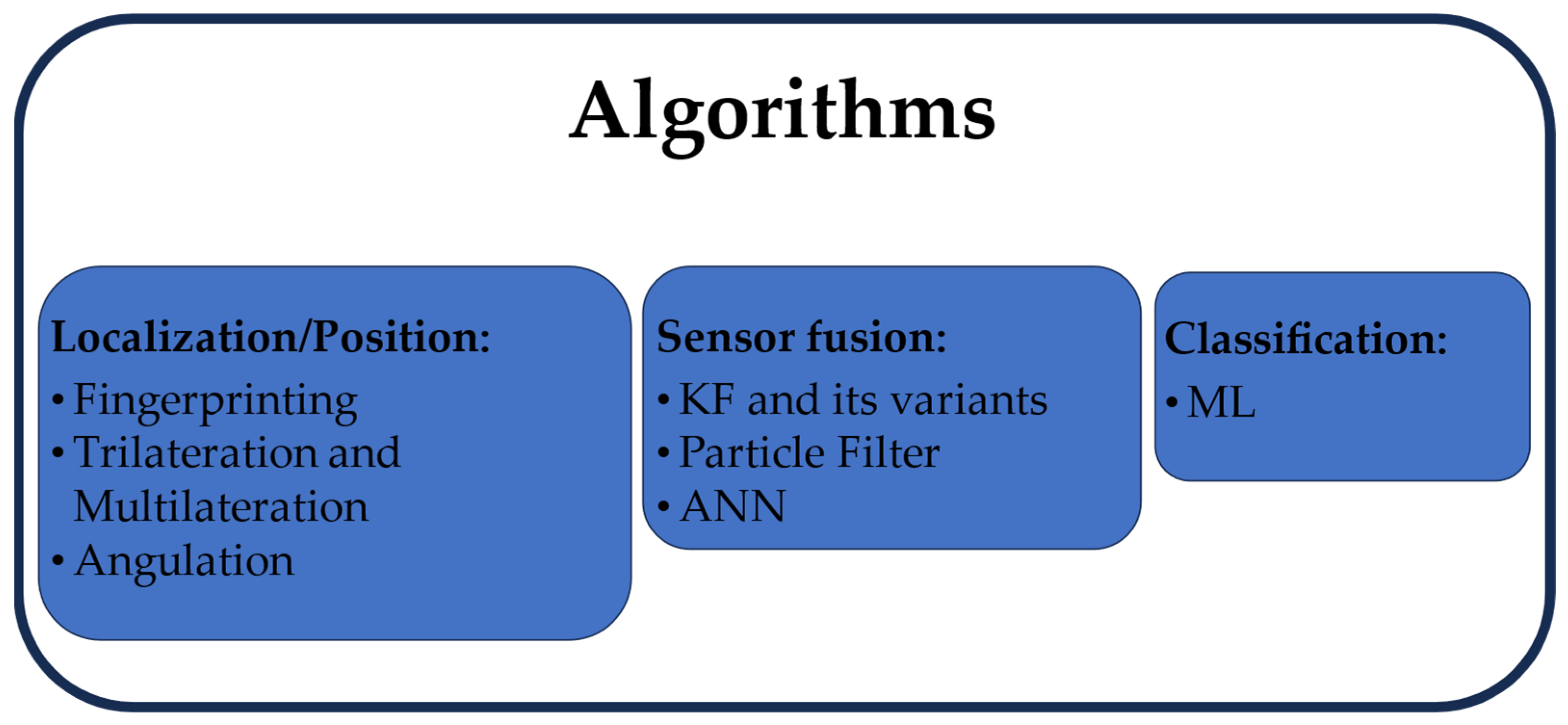
