Article

Classification of Whole-Slide Pathology Images Based on State Space Models and Graph Neural Networks

1
School of Automation, Nanjing University of Information Science and Technology, Nanjing 210044, China
2
College of Information Engineering, TaiZhou University, Taizhou 225300, China
3
Jiangsu Key Laboratory of Intelligent Medical Image Computing, School of Artificial Intelligence, Nanjing University of Information Science and Technology, Nanjing 210044, China
4
Department of Radiology, Nanjing First Hospital, Nanjing Medical University, Nanjing 211112, China
*
Author to whom correspondence should be addressed.
These authors contributed equally to this work.
Electronics 2025, 14(10), 2056; https://doi.org/10.3390/electronics14102056
Submission received: 2 April 2025 / Revised: 8 May 2025 / Accepted: 12 May 2025 / Published: 19 May 2025
(This article belongs to the Special Issue AI-Driven Medical Image/Video Processing)

Abstract

:
Whole-slide images (WSIs) pose significant analytical challenges due to their large data scale and complexity. Multiple instance learning (MIL) has emerged as an effective solution for WSI classification, but existing frameworks often lack flexibility in feature integration and underutilize sequential information. To address these limitations, this work proposes a novel MIL framework: Dynamic Graph and State Space Model-Based MIL (DG-SSM-MIL). DG-SSM-MIL combines graph neural networks and selective state space models, leveraging the former’s ability to extract local and spatial features and the latter’s advantage in comprehensively understanding long-sequence instances. This enhances the model’s performance in diverse instance classification, improves its capability to handle long-sequence data, and increases the precision and scalability of feature fusion. We propose the Dynamic Graph and State Space Model (DynGraph-SSM) module, which aggregates local and spatial information of image patches through directed graphs and learns global feature representations using the Mamba model. Additionally, the directed graph structure alleviates the unidirectional scanning limitation of Mamba and enhances its ability to process pathological images with dispersed lesion distributions. DG-SSM-MIL demonstrates superior performance in classification tasks compared to other models. We validate the effectiveness of the proposed method on features extracted from two pretrained models across four public medical image datasets: BRACS, TCGA-NSCLC, TCGA-RCC, and CAMELYON16. Experimental results demonstrate that DG-SSM-MIL consistently outperforms existing MIL methods across four public datasets. For example, when using ResNet-50 features, our model achieves the highest AUCs of 0.936, 0.785, 0.879, and 0.957 on TCGA-NSCLC, BRACS, CAMELYON16, and TCGA-RCC, respectively. Similarly, with UNI features, DG-SSM-MIL reaches AUCs of 0.968, 0.846, 0.993, and 0.990, surpassing all baselines. These results confirm the effectiveness and generalizability of our approach in diverse WSI classification tasks.

1. Introduction

Pathological analysis serves as the foundation for disease diagnosis, staging, and treatment decision making [1]. Pathologists diagnose and classify various diseases by examining tissue samples under a microscope, particularly in the context of cancer. Early cancer detection relies on the comprehensive interpretation of cellular morphology, tissue architecture, and molecular markers. Traditional pathological analysis methods primarily depend on visual inspection and pathologists’ expertise. Although these methods have been refined over many years, they remain time-consuming and susceptible to variability due to individual experience, technical proficiency, and subjective bias, which can affect the accuracy and consistency of diagnoses [2,3].
In recent years, with the widespread adoption of whole-slide images (WSIs), the field of pathology has gradually transitioned toward computer-aided diagnosis (CAD) [4]. The digitization of WSIs allows tissue samples to be captured in high resolution, facilitating automated and large-scale analysis. However, WSI analysis poses two major technical challenges for conventional deep learning models: (1) the gigapixel resolution of WSI exceeds the computational capacity of standard hardware for end-to-end processing [5], and (2) supervised learning tasks such as image segmentation typically require pixel-level annotations, which are labor-intensive, costly, and often unavailable in clinical datasets [6].
To address these challenges, multiple instance learning (MIL)—a weakly supervised learning paradigm—has emerged as a core method in computational pathology. MIL assumes that a WSI (i.e., a “bag”) is labeled positive if it contains at least one diseased region (i.e., a “positive instance”) and negative if all regions are normal. This formulation closely aligns with clinical practice, where slide-level diagnoses (e.g., “cancer” or “normal”) are commonly available, but fine-grained annotations (e.g., tumor boundaries) are rarely provided. Deep learning further enhances the power of MIL by automating feature extraction and capturing complex patterns. For instance, convolutional neural networks (CNNs) can extract discriminative features from image patches (instances), while graph neural networks (GNNs) model spatial relationships among patches [7].
Typically, image patches are transformed into low-dimensional features using a pretrained model, and the features of all patches within the entire WSI are then aggregated for further analysis [8]. Under this paradigm, MIL reformulates the WSI classification task as a long-sequence modeling problem. Since the instance aggregation process directly affects the discriminative power of bag-level features—and consequently impacts model performance—many MIL frameworks focus on improving this aggregation step. For example, ABMIL [9] incorporates an attention mechanism to selectively focus on the most relevant instances, enhancing MIL task performance. The CLAM [10] model introduces clustering constraints on instances to reduce reliance on large-scale data. DTFDMIL [11] adopts a pseudo-bag strategy to alleviate overfitting caused by the limited number of WSIs. DSMIL [12] employs a dual-stream architecture to simultaneously capture instance-level and bag-level information, addressing the decision boundary shift problem caused by the imbalance between positive and negative instances in MIL. However, the above methods treat each instance as independent and identically distributed, ignoring the contextual relationships among instances. To address this, models such as TransMIL [13], MCAT [14], and Dt-MIL [15] leverage Transformer [16] to explore interinstance correlations and model long-range dependencies.
Building on these insights, we propose the Dynamic Graph and State Space Model-Based MIL (DG-SSM-MIL) framework. This MIL architecture combines GNNs with the Mamba model, fusing the local information captured by the GNN with the global context encoded by Mamba for whole-slide image classification. The Mamba model, introduced by Gu et al. [17], is centered on a selective state space model (selective SSM) mechanism. This mechanism dynamically adjusts the state transition parameters, enabling the model to selectively focus on critical information based on the input content, thereby significantly improving the efficiency and performance of long-sequence modeling. This capability is particularly valuable for multi-instance analysis of pathological whole-slide images, where lesion regions are often discontinuous and spatially dispersed, posing challenges for reliable prediction. Previous studies have shown that preserving fine-grained details in pathology images is crucial and directly contributes to improved diagnostic accuracy [18]. Consequently, we employ the Mamba model as our long-sequence encoder to capture long-range contextual information across patches and enhance diagnostic reliability.
DG-SSM-MIL divides the patch feature sequences extracted by a pretrained model into two parallel paths: one path retains the original features, while the other path uses a GAT to extract spatial and local information from the image patches. These two paths are then input into a Dynamic Graph and State Space Model (DynGraph-SSM) module, and the updated features are subsequently fed into the MIL module for aggregation and image classification. Notably, Hayat et al. emphasized that, in medical image analysis, preserving fine-grained details and modeling global structures are equally important, and their integration contributes positively to classification performance [19]. The DynGraph-SSM module consists of a dynamic graph structure and a Bidirectional State Space Model for Vision (Bi-SSM-vision) module. The outputs from the two paths are integrated within the dynamic graph module to incorporate spatial and local information into the original feature sequence. This attention-based fusion process helps effectively address the issue of dispersed lesion distribution in pathological images and mitigates, to some extent, the limitation of Mamba’s unidirectional scanning. The updated features are then passed into the Bi-SSM-vision module. To better adapt to image classification tasks, we replace the 1D causal convolution used in the original Bi-SSM [20] with standard 1D convolution, allowing effective extraction of global information in both forward and backward directions. Additionally, we create a symmetric branch without SSM to extract local features from the updated representations further. Finally, the output of the DynGraph-SSM module is sent to the MIL module for final aggregation and image classification. The main contributions of this paper can be summarized as follows:
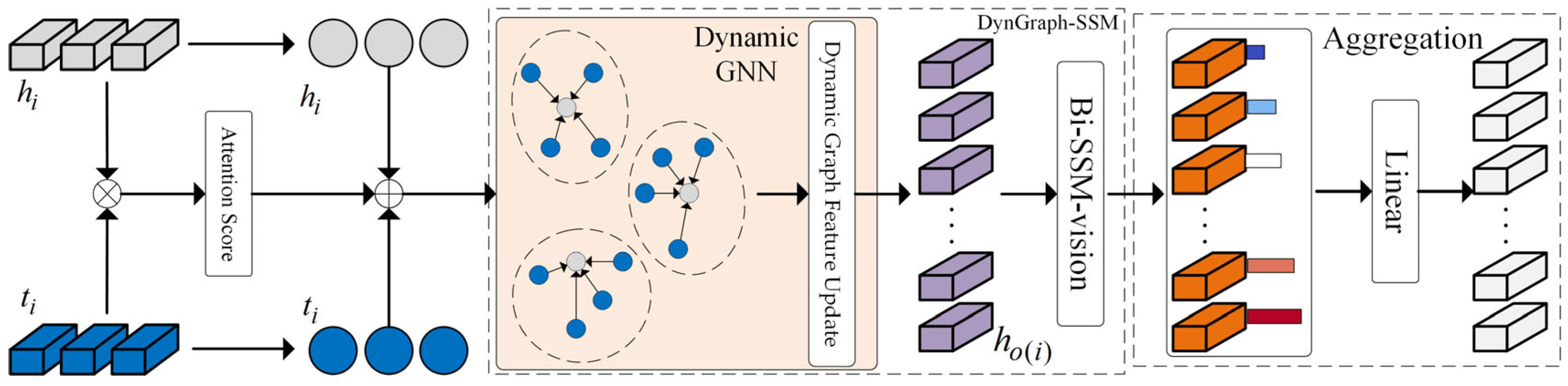
  • We propose the DG-SSM-MIL framework, which consists of two parallel paths. The input feature vectors are separately fed into the DynGraph-SSM module as original features and GAT-processed features. This design enables more effective fusion of local and global information, allowing the model to better capture the spatial structure and interrelationships of image patches, thereby enhancing the multidimensional expressiveness of features and significantly improving their completeness and robustness.
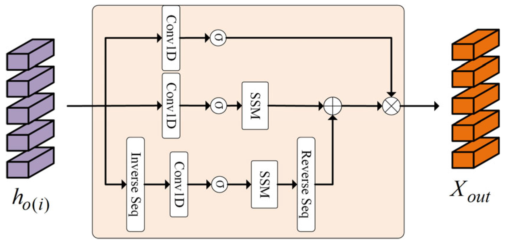
  • We combine static and dynamic graph structures, enabling the model to more effectively capture correlations among positive regions and alleviate the limitation of Mamba’s unidirectional scanning, thereby improving classification performance. Meanwhile, we propose the Bi-SSM-vision module, an improved version of Bi-SSM tailored for image tasks. In this module, the original 1D causal convolutions are replaced with standard 1D convolutions to enhance compatibility with image processing. Additionally, we introduce an extra convolutional branch to extract local features from the dynamically updated representations, enabling joint modeling of local patterns and Mamba’s long-sequence modeling capabilities.
  • We validate the model’s superior performance across multiple challenging tasks and datasets. Through extensive experiments on several public medical image datasets, including BRACS [21], NSCLC, RCC, and CAMELYON16 [22], our model demonstrates strong robustness and broad applicability. The results show that the improved model can leverage local and global information more effectively to enhance predictive performance.

2. Related Works

2.1. Graph Neural Networks

A graph is a data structure that represents a set of objects (nodes) and the relationships (edges) between them. In recent years, due to its strong capacity to model complex systems across various domains, graph-based deep learning has attracted increasing attention [23]. These domains include the social sciences (e.g., social networks), natural sciences (e.g., physical systems and protein–protein interaction networks), knowledge graphs, and other research areas. Many real-world problems can be naturally modeled as graphs, where nodes denote entities and edges capture the relationships or interactions between them [24]. For example, a molecule can be represented as a graph where nodes correspond to atoms and edges represent chemical bonds. Similarly, a biomedical knowledge graph can connect hundreds of thousands of genes, drugs, and diseases, where each is a node in the graph [25]. A graph is typically denoted as G = V , E , where V is the set of nodes and E is the set of edges. For two adjacent nodes u and v, the edge between them is denoted as e = u , v . Edges can be either directed or undirected: in the former case, the graph is called a directed graph; in the latter, it is referred to as an undirected graph [26].
To effectively learn from graph-structured data, graph neural networks (GNNs) have emerged as a powerful deep learning paradigm. Unlike traditional models, GNNs leverage a message passing mechanism, where information from neighboring nodes is iteratively aggregated to compute node- or graph-level representations. This enables GNNs to capture rich topological and relational structures within the graph [27]. Typical tasks supported by GNNs include node classification, link prediction, and graph classification.
In recent years, various GNN variants have been proposed to accommodate different tasks and scenarios. For instance, graph convolutional networks (GCNs) simplify graph convolution through spectral methods; graph attention networks (GATs) enhance model flexibility by incorporating attention mechanisms; and dynamic graph neural networks (e.g., EvolveGCN) are designed to handle graphs whose structures evolve over time [28,29]. Additionally, sampling and pooling modules have enabled GNNs to scale to large-scale graph data.
To transform a pathological image into a graph structure, as illustrated in Figure 1, the process involves dividing the WSI into multiple image patches and representing each patch as a node in the graph. The connections (edges) between nodes are typically established based on spatial proximity, feature similarity, or other contextual information. For example, Shi et al. [30] treated the WSI as a graph, where each patch serves as a node and edges are constructed based on spatial positions using the k-nearest neighbors (k-NN) algorithm. This approach enables the model to capture spatial relationships between patches, thereby improving classification performance, and it is the method we adopt for GAT-based graph construction in our experiments. Guan et al. [31] proposed a node-aligned graph convolutional network that constructs directed graphs to enhance interactions between patches and employs a global clustering strategy to establish node correspondences across different WSIs, enabling more effective WSI representation and classification. Adnan et al. [32] modeled the WSI as a fully connected graph, where the adjacency matrix was learned in an end-to-end fashion. They combined graph convolutional networks with attention-based pooling to perform representation learning, achieving efficient subtype classification of lung cancer.
The GNN has been widely applied in diverse domains such as social networks, knowledge graphs, molecular modeling, and traffic prediction. Despite significant progress, challenges remain in areas such as ultra-large-scale graph processing, dynamic graph modeling, and theoretical understanding —highlighting the vast potential for future research [33].

2.2. Application of Multiple Instance Learning in WSI Classification

Clinical practice heavily relies on pathologists to manually annotate and analyze pathological images, a traditional approach that is time-consuming, labor-intensive, and prone to subjective variability. To address these challenges, multiple instance learning (MIL) has emerged as a prominent method for whole-slide image (WSI) classification, particularly under weakly supervised settings [34]. WSI typically consists of high-resolution tissue slides containing numerous local image regions (i.e., “instances”), which exhibit significant heterogeneity and complexity. Traditional supervised learning methods are difficult to apply in this context, as they usually require precise pixel-level annotations, which are often unavailable in WSIs. MIL offers a solution by training models using only bag-level labels [35].
The application of MIL in WSI classification can be broadly categorized into two types. Instance-level approaches aim to infer pseudo-labels for individual instances based on bag-level supervision. These methods train an instance-level classifier to score each instance and then aggregate the top-k highest-scoring instances to produce the final bag-level prediction. The advantage of this approach lies in its ability to focus directly on critical regions, such as tumor areas with high diagnostic value. However, instance-level methods have limitations—they typically require large amounts of WSI data for training, as only a small number of instances per slide contribute to learning [36].
On the other hand, embedding-level approaches map each instance to a fixed-length embedding space and aggregate these embeddings (e.g., via max or average pooling) to represent the entire bag. These methods often incorporate trainable attention mechanisms to assign weights to each instance, thereby enabling more accurate and informative aggregation. Additionally, feature clustering methods represent the entire bag by computing the cluster centers of all instance embeddings, reducing noise and improving classification performance [37].
Despite the strong adaptability of MIL for WSI classification, several challenges remain. Instance-level approaches are susceptible to the influence of misclassified instances and require large datasets. While embedding-level methods better handle data heterogeneity, they still struggle to capture complex, long-range dependencies between instances. To overcome these limitations, recent studies have introduced new techniques such as non-local attention mechanisms and self-supervised contrastive learning to enhance model robustness. With these advancements, the performance of MIL methods in WSI classification tasks continues to improve [38].

2.3. Mamba: Evolution of State Space Models Based on Selective Mechanisms

A state space model (SSM) is a mathematical model used to describe dynamic systems with inputs, outputs, and internal states. In an SSM, the behavior of the system is defined by a set of linear or non-linear equations that describe the temporal evolution of the system’s state and how the output is derived from it [39]. The state space representation is widely used in control theory, signal processing, time series analysis, and various engineering applications. It maps a one-dimensional input signal x t to a one-dimensional output signal y t , as defined in Equation (1):
h ( t ) = A h ( t ) + B x ( t ) y ( t ) = C h ( t )
where A R N × N is the state matrix, and B R N × 1 and C R N × 1 are projection parameters. This representation enables the model to capture complex relationships between the input x t and output y   t through the latent state h t . State space models (SSMs) were originally designed for continuous signals. However, in most model applications, the inputs are discrete (such as text sequences), which necessitates discretizing the model. To achieve this, the zero-order hold (ZOH) technique is applied. Each time a discrete input is received, its value is held constant until the next discrete input arrives. The symbol Δ represents the discretization step, indicating the time interval between samples. This process effectively generates a continuous signal from the discrete inputs.
To adapt the model to deep learning scenarios with discrete inputs, various discretization rules can be applied to the parameters in Equation (1) using the step size Δ , which represents the sampling interval of the continuous input x t . This process transforms the continuous parameters A and B into discrete counterparts A ¯ and B ¯ . These discrete parameters are typically computed using the ZOH rule, as shown in Equation (2):
A ¯ = exp ( Δ A ) B ¯ = ( Δ A ) 1 ( exp ( Δ A ) I ) · Δ B
The discretized parameters enable the SSM to be used for autoregressive inference in a recurrent manner, with the computation defined as shown in Equation (3):
h t = A ¯ h t 1 + B ¯ x t y t = C h t
However, the recurrent formulation is suboptimal for training, as it processes tokens sequentially. Therefore, researchers aim to parallelize the computation as much as possible to ensure high efficiency, similar to how the Transformer model operates. Fortunately, state space models also offer a convolutional form, which can be expressed as shown in Equation (4):
K = ( C B ¯ , C A ¯ B ¯ , , C A ¯ M 1 B ¯ ) y = x K
Building upon traditional SSMs, the structured state space sequence model (S4 model) leverages the HiPPO framework to encode historical information into a low-dimensional state, allowing it to capture long-term dependencies in continuous-time settings. However, its time-invariant nature limits its adaptability to different inputs [40]. Specifically, Mamba introduces selection mechanisms that allow the model parameters to depend on the input features. At the same time, it utilizes hardware-aware parallel algorithms to optimize computational efficiency. This selection mechanism enables Mamba to selectively propagate or forget information during sequence modeling based on the characteristics of the current input, significantly improving the efficiency of handling long sequences. The combination of Mamba’s selective state space approach, hardware-aware algorithms, and simplified architecture makes it a powerful and versatile option for a wide range of sequence modeling tasks.
Since the parameters in Mamba are time-varying, it cannot use convolution for computation, which prevents it from performing fully parallel computation. The only viable approach is a recurrent formulation [41]. However, the Mamba model addresses this limitation by introducing a parallel scan algorithm, which allows its recurrent computations to be parallelized. This parallel scan algorithm defines a new computational operation, as shown in Equation (5):
( A t , B t x t ) ( A t + 1 , B t + 1 x t + 1 ) = ( A t A t + 1 , A t + 1 B t x t + B t + 1 x t + 1 )
In addition, Mamba incorporates a hardware-aware algorithm to accelerate computation, leveraging three classic optimization techniques: parallel scan, kernel fusion, and recomputation. Through these enhancements, the Mamba framework demonstrates outstanding performance in tasks that require efficient processing of long-sequence data, such as natural language processing, time series forecasting, and pathology image analysis. The model can capture long-range dependencies at a relatively low computational cost and effectively addresses the challenges posed by large-scale data [42]. Therefore, this paper uses Mamba to extract global information from feature vectors instead of using a transformer.

3. Methods

3.1. Framework Overview

Figure 2a illustrates the overall feature extraction pipeline. First, to eliminate irrelevant regions, the Otsu thresholding algorithm [43] is applied to detect and remove background areas in the WSI. In a large-scale WSI (gigapixel images), failure to exclude the background regions may result in significant computational overhead. Next, the WSI is divided into 512 × 512 pixel patches at 20× magnification. These patches are then processed using pretrained ResNet-50 [44] and UNI [45] models to extract 1024-dimensional feature vectors. This process generates an instance feature sequence X = x 1 , x 2 , x 3 , , x L , where x i R D represents an instance feature, L is the sequence length, and D is the feature dimension. Subsequently, X undergoes linear projection for dimensionality reduction. Finally, the processed low-dimensional features are fed into the DG-SSM-MIL framework to generate a bag-level representation for downstream classification tasks.
Unlike typical visual modalities, WSIs contain sparse and scattered positive patches with weak spatial correlation. This makes them well-suited for Mamba’s powerful sequence modeling capabilities. Mamba is designed for long-range dependency modeling and is renowned for its computational efficiency based on state space models (SSMs), excelling at capturing global contextual information effectively. We propose the DG-SSM-MIL framework to fully leverage Mamba’s strength in modeling global context while incorporating the advantages of GNNs in capturing local and spatial information. In this framework, the feature sequence extracted by a pretrained model is fed into two separate paths. The first path maintains the original sequence structure, while the second rearranges the sequence according to the spatial layout of the WSI and constructs it into a graph, where each patch is treated as a node. Edges in the graph are constructed using the k-nearest neighbors (k = 8), with Euclidean distance between nodes as the similarity metric (Figure 2c). Neighboring patches provide contextual cues to each other and share information. A graph neural network is then applied to extract local features and spatial structural information from this graph-based representation.
The feature vectors generated from the two paths are subsequently fed into our proposed DynGraph-SSM module, as illustrated in the schematic diagram in Figure 2d. This module consists of two components: a dynamic graph module and a Bi-SSM-vision module. First, the dynamic graph module takes as input the outputs from both paths and integrates the features extracted by the GAT module from the second path into the original feature sequence, thereby effectively embedding local and spatial structural information into the original features. The updated feature vectors are then passed into the Bi-SSM-vision module, which extracts features in both forward and backward directions, enabling it to capture global contextual information and sequential dependencies across long sequences. In addition, a non-SSM branch is incorporated to further extract local information from the updated features using a convolutional network. Although the Bi-SSM-vision module mitigates the limitations of unidirectional scanning to some extent through the use of bidirectional feature extraction, each individual scanning direction (forward or backward) remains inherently unidirectional and cannot perceive “future” information during its pass. To address this issue, the preceding dynamic graph module employs an attention mechanism to select the k most important neighboring nodes, allowing information from future patches to be integrated into the current patch in advance, while also helping to alleviate the issue of dispersed tumor regions. This mechanism helps to alleviate the shortcomings of purely sequential modeling. Finally, the output feature sequence from the Bi-SSM-vision module is passed into a lightweight MIL module, as shown in Figure 3, where it is further aggregated into a bag-level representation for WSI classification.

3.2. Graph Attention Network (GAT) Module

In this study, we employ a graph attention network (GAT) to perform initial local feature extraction. GAT utilizes an attention mechanism to dynamically learn the relative importance of neighboring nodes, allowing the network to focus on the most semantically relevant regions. As illustrated in Figure 2c, each patch feature vector is modeled as a node within a graph, with edges constructed using the k-nearest neighbors (k-NN) algorithm. Following the methodologies of Ding et al. [46] and Chen et al. [47], we set k = 8 to emulate the local receptive field of a 3 × 3 convolutional kernel in CNNs, thereby enabling the capture of local contextual information. These studies have shown that adjacent patches can provide valuable context for one another and effectively share informative features. To preserve spatial coherence, nodes are arranged according to their original spatial locations in the WSI, which facilitates efficient message passing between anatomically adjacent regions.
In the constructed GAT network, each node is connected to its eight nearest neighbors based on Euclidean distance. GAT applies a self-attention mechanism to perform weighted aggregation of neighboring nodes for each target node, generating updated node representations. By dynamically adjusting the aggregation based on relative importance between nodes, GAT offers high flexibility and can effectively capture local information—such as spatial dependencies—without relying on global structural information.
Specifically, the WSI is divided into 512 × 512 pixel patches at 20× magnification. These patches are passed through a pretrained model to extract a 1024-dimensional feature sequence X . After dimensionality reduction via a linear layer, the resulting features H are rearranged based on their original spatial layout in the WSI, with each patch corresponding to a node in the graph. Then, each node is connected to its eight nearest neighbors using Euclidean distance, forming the edges and completing the graph structure. This graph is subsequently fed into the GAT network for feature updating, producing the enhanced feature sequence T .

3.3. Dynamic Graph and State Space Model (DynGraph-SSM) Module

As shown in Figure 2b, the feature sequence H extracted by the pretrained model and the feature sequence T , which has been enriched with local features and spatial information through the GAT module, are processed by the DynGraph-SSM module after computing attention scores. The processed features are then fed into the MIL module, where they are aggregated into a bag-level representation for image classification. The DynGraph-SSM module consists of two main components. The design of its dynamic graph component draws inspiration from the attention-aware graph structures introduced by Li et al. [48] and Xiang Wang et al. [49], which emphasize adaptive message propagation based on internode relevance. First, the sequences H and T are passed through a dynamic graph structure, where each feature vector h i and t i is treated as an individual node in the graph. The purpose of this dynamic graph is to facilitate sufficient interaction between the two feature sequences, allowing the local and spatial information in T to be effectively integrated into H through attention-based message passing. Next, the updated sequence h O i is fed into the Bi-SSM-vision module, a key component of the framework. This module leverages the Mamba model’s capability to effectively model long-range dependencies. Taking as input the feature vectors that have already incorporated local and spatial information, Bi-SSM-vision processes the sequence in both forward and backward directions to capture sequential dependencies and long-range contextual information. In addition, a non-SSM branch is introduced to further enhance local feature extraction. Through this design, the module achieves more effective integration of local and global features, enabling more accurate and robust image classification.

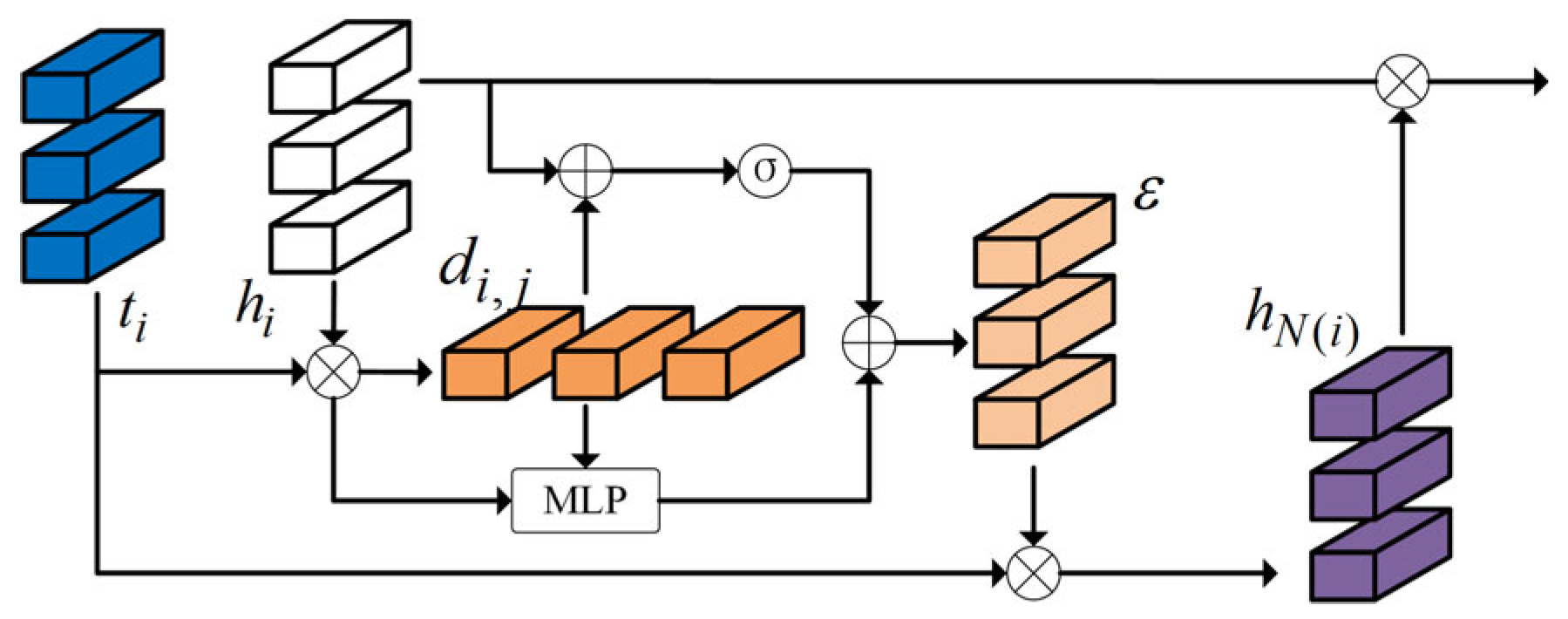
3.3.1. Dynamic Graph Structure

First, the sequences H and T are passed through a dynamic graph structure, where each feature vector h i and t i is treated as an individual node in the graph. This dynamic graph facilitates sufficient interaction between the two sequences, allowing the local and spatial information contained in T to be effectively integrated into H through attention-based message passing. At the same time, this mechanism also helps to address the issue of dispersed tumor regions, allowing future information to be incorporated into the current feature vectors to some extent. This enables the subsequent Bi-SSM-vision module to capture both sequentially dependent features and order-independent features, which helps alleviate the limitation of unidirectional information flow in the Bi-SSM-vision module to some extent.
Specifically, the dot-product similarity is first computed between each pair of feature vectors from H and T , followed by a softmax function to calculate the normalized similarity between h i and t j . The computation is illustrated in Equation (6):
ω i , j = exp ( h i T t j ) j = 1 N exp ( h i T t j )
where h i denotes the i t h feature vector in the feature sequence H and t j denotes the j t h feature vector in the feature sequence T . The term ω i , j represents the similarity score between h i and t j . Subsequently, the feature vectors from H and T , along with their corresponding attention scores, are fed into the dynamic graph structure of the DynGraph-SSM module, where h i and t j serve as the nodes in the graph. For each original feature vector h i (corresponding to a patch), the top-k most similar feature vectors from T are selected as its neighboring nodes based on the similarity scores. The selection is as shown in Equation (7):
N ( i ) = j V : ω i , j T o p k ω i , j j = 1 N
where V represents the total number of feature vectors in the feature sequence T and T o p k ω i , j j = 1 N denotes the top-k similarity scores selected from all ω i , j between h i and t j . N i represents the index set of the k most similar nodes to h i , i.e., the top-k nodes in T with the highest similarity scores; by definition, N i = k . In our experiments, k is set to 6. The feature update process of the dynamic graph is illustrated in Figure 4. In this structure, directed edges are assigned edge features, which are computed based on h i and t j as shown in Equation (8):
d i , j = ω i , j t j + ( 1 ω i , j ) h i
where d i , j represents the edge feature from the j t h feature vector in sequence T to the i t h feature vector in sequence H , and each j belongs to the set N i . This equation also defines how the edges are constructed in the dynamic graph: an edge is established from t j to h i , indicating a directed connection from t j to h i . Afterward, the feature vectors are updated through message passing between nodes, leading to the final output. The weighted aggregation of neighbor information is computed as shown in Equation (9):
h N ( i ) = j N ( i ) θ ( h i , d i , j , t j ) t j , ( i j )
where θ is a weight score that determines the contribution of each neighboring node to the update of h i , and h N i is the aggregated feature representation obtained from the k neighboring nodes corresponding to h i . The weight score θ is normalized by ε, which is computed as shown in Equation (10):
ε ( h i , d i , j , t j ) = ( 1 λ ) t j T tanh ( h i + d i , j ) + λ M L P ( h i , d i , j , t j )
Subsequently, the ε is normalized using the softmax function:
θ ( h i , d i , j , t j ) = exp ( ε ( h i , d i , j , t j ) ) j N ( i ) exp ( ε ( h i , d i , j , t j ) )
By adopting the above neighbor node aggregation method, h i can capture information from its neighboring nodes effectively. Finally, the aggregated neighbor information is fused with the original feature vector h i through element-wise multiplication and summation operations to obtain the final output vector of the dynamic graph. The specific computation is as shown in Equation (12):
h O ( i ) = α ( w 1 ( h i + h N ( i ) ) ) + β ( w 2 ( h i h N ( i ) ) )
where h O i is the updated feature vector of h i after processing through the dynamic graph structure, α and β denote activation functions, and w 1 and w 2 are learnable transformation matrices. Through the feature aggregation in the dynamic graph, h O i integrates local and spatial information on top of the original feature representation. Subsequently, h O i is used as the input sequence to the Bi-SSM-vision module.

3.3.2. Bidirectional State Space Model for Vision (Bi-SSM-Vision) Module

The output h O i generated by the dynamic graph structure is used as the input to the Bi-SSM-vision module. Within the DynGraph-SSM module, Bi-SSM-vision serves as a critical component that fully leverages the Mamba model’s capability to capture global relationships and long-range dependencies across a large number of instances. This module extracts features from both the forward and backward directions of the sequence, resulting in global sequential dependencies in both directions. However, such sequential scanning conflicts with the inherently dispersed distribution of lesions in pathological images. Fortunately, the preceding dynamic graph module has already embedded future information into the original features in advance. As a result, when Bi-SSM-vision processes the updated feature sequence, it can still learn non-sequential dependencies, thereby enabling more accurate localization of spatially scattered lesions. As illustrated in Figure 5, the Bi-SSM-vision module consists of a bidirectional SSM path and a non-SSM convolutional path. The non-SSM convolutional path performs local feature extraction on the updated h O i , and the resulting features are combined with the global features captured by the bidirectional SSM path. This design enhances the interaction between local and global features, ultimately improving classification performance. The computation process is illustrated in the pseudocode of Algorithm 1.
Algorithm 1 Bi-SSM-vision Module Process
Input: instance sequence h O i :(B,S,D)
Output: instance sequence X o u t :(B,S,D)
 # B: batch size, S:instance number, D: dimension
h O i :   ( B , S , D )     LayerNorm ( h O i )
 #Forward Sequence: for
X f o r   :   ( B , S ,   D   )     L i n e a r x 0 h O i
 #Backward Sequence: back
X b a c k   :   ( B , S ,   D   )     F l i p x 1 X f o r
 # Convolutional Path: conv
X c o n v : ( B , S ,   D   )     X f o r
for o in {for,back} do
Z o :   ( B , S ,   D   )     SiLU ( L i n e a r z ( X ))
   X o : ( B , S ,   D   )     SiLU ( C o n v 1 d o ( X ))
   B o : ( B , S , N )     L i n e a r B X o
   C o : ( B , S , N )     L i n e a r C X o
   Δ o : ( B , S ,   D   )     softplus ( L i n e a r Δ X o )
   A o ¯ : ( B , S ,   D   , N )     d i s c r e t i z e A Δ , A o
   B o ¯ : ( B , S ,   D   , N )     d i s c r e t i z e B Δ , A o , B o
   y o : ( B , S ,   D   )     SSM ( A o ¯ , B o ¯ , C o ) ( X o )
end for
y f o r :   ( B , S ,   D   )     y f o r SiLU ( Z f o r ) ,   y b a c k :   ( B , S ,   D   )     y b a c k SiLU ( Z b a c k )
y c o n v :   ( B , S ,   D   )     SiLU ( Conv 1 d ( X c o n v ))
X o u t :   ( B , S , D )     Linear ( y f o r + y b a c k + y c o n v )
return X o u t
In this work, the proposed Bi-SSM-vision module is built upon the original SSM architecture. To better adapt it to vision tasks, the original 1D causal convolution is replaced with a standard 1D convolution. The output of the dynamic graph module serves as the input to this module, as shown in Equation (13):
X f o r = h O ( i ) X c o n v = h O ( i ) X b a c k = F l i p ( h O ( i ) )
where X c o n v represents the forward feature input of the first path in the Bi-SSM-vision module, X f o r denotes the forward feature input of the second path, and X b a c k denotes the reverse feature input of the third path. Subsequently, these inputs are processed as shown in Equation (14):
X f o r = S S M ( s i l u ( C o n v 1 D ( L i n e a r ( X f o r ) ) ) ) X c o n v = s i l u ( C o n v 1 D ( L i n e a r ( X f o r ) ) ) X b a c k = S S M ( s i l u ( C o n v 1 D ( L i n e a r ( X b a c k ) ) ) )
where X f o r represents the output of the forward feature X f o r after being processed by the selective state space model, X c o n v denotes the result of applying a 1D convolution to the forward feature X f o r , and X b a c k represents the output of the reverse feature X b a c k after passing through the selective state space model. S S M refers to the internal computation formulas of the Mamba model introduced in the Related Works section, detailed in Algorithm 1. These three outputs are then aggregated to obtain a new feature sequence, as defined in Equation (15):
X o u t = L inear ( X f o r + X b a c k + X c o n v )
where X o u t is the final output of the Bi-SSM-vision module, obtained by adding X f o r , X b a c k , and X c o n v and passing them through a linear layer, resulting in the final output of the DynGraph-SSM module.

4. Experiments and Analysis

4.1. Experimental Setup

An early stopping strategy was adopted, and the experiments were conducted on a workstation running Ubuntu 22.04.4 LTS with an NVIDIA RTX 4090 GPU (NVIDIA Corporation, Santa Clara, CA, USA). The model was trained for 200 epochs. During training, we used the Adam optimizer with a learning rate of 2 × 10⁻⁴ and a weight decay of 1 × 10⁻⁵. For feature extraction, we employed ResNet-50 pretrained on ImageNet-1K, as well as UNI, a backbone model pretrained on over 100,000 Hematoxylin and Eosin (H&E)-stained WSIs.

4.2. Datasets

To validate the effectiveness of our proposed method, we conducted cancer detection and subtype classification experiments on four datasets, all of which were obtained through legitimate sources and are open access. The dataset links are provided at the end of the paper. To assess the generalization and robustness of our approach, we extracted two sets of features using ResNet-50 pretrained on ImageNet [50] and UNI, a backbone model pretrained on over 100,000 H&E-stained WSIs.
We evaluated our method on the CAMELYON16, BRACS, TCGA-NSCLC, and TCGA-RCC datasets for cancer diagnosis and subtype classification tasks. CAMELYON16 is a dataset for breast cancer metastasis diagnosis, containing 399 WSIs, classified into two categories: Normal and Tumor. TCGA-NSCLC includes two non-small cell lung cancer (NSCLC) subtypes: Lung Adenocarcinoma (LUAD) and Lung Squamous Cell Carcinoma (LUSC). Specifically, LUAD consists of 541 slides from 478 patients, and LUSC contains 512 slides from 478 patients. BRACS comprises 545 WSIs collected from 189 patients, divided into seven categories: Normal (N), Pathological Benign (PB), Usual Ductal Hyperplasia (UDH), Flat Epithelial Atypia (FEA), Atypical Ductal Hyperplasia (ADH), Ductal Carcinoma In Situ (DCIS), and Invasive Carcinoma (IC). TCGA-RCC is divided into three classes: Kidney Chromophobe (TCGA-KICH), Kidney Clear Cell Carcinoma (TCGA-KIRC), and Kidney Papillary Cell Carcinoma (TCGA-KIRP). This dataset contains a total of 884 diagnostic WSIs, including 111 KICH slides from 99 patients, 489 KIRC slides from 483 patients, and 284 KIRP slides from 264 patients.

4.3. Evaluation Metrics

For cancer diagnosis and subtyping tasks, we adopted 10-fold Monte Carlo cross-validation, splitting the data into training, validation, and test sets in a ratio of 8:1:1. To evaluate the performance of our method on these tasks, we used area under the curve (AUC) and accuracy (ACC) along with their standard deviation (std). These metrics provide a robust evaluation approach that is less sensitive to class imbalance. In statistics and machine learning, the AUC is widely used to evaluate the performance of binary classification models. It represents the area under the receiver operating characteristic (ROC) curve, which plots the false positive rate (FPR) on the x-axis and the true positive rate (TPR) on the y-axis. The ROC curve was originally used during World War II in electrical and radar engineering for military target detection tasks [51]. Since then, it has been widely adopted in fields such as psychology, medicine, and machine learning for model performance evaluation.
In medical image classification tasks, the ROC curve depicts the trade-off between TPR and FPR across different decision thresholds, enabling clinicians to select an operating point that best matches specific clinical requirements. For instance, physicians often wish to know the FPR when the sensitivity—i.e., TPR—reaches 95%; the ROC curve provides a direct visual aid for such decisions and is therefore more informative and interpretable than the single-value AUC alone. Furthermore, the ROC curve can expose latent performance deficiencies. In some cases, a model with a high AUC may still produce a ROC curve that is jagged, contains multiple inflection points, or shows local performance drops, indicating instability for certain data distributions or threshold regions. These fine-grained details are essential for diagnosing model weaknesses and guiding further architectural improvements. The formulas for calculating FPR and TPR are as shown in Equation (16):
F P R = F P F P + T N T P R = T P T P + F N
where FP represents false positives, referring to the number of negative samples that are incorrectly classified as positive; TN represents true negatives, which are the number of samples correctly classified as negative. FPR is the proportion of negative samples that are incorrectly classified as positive. TP stands for true positives, referring to the number of samples correctly classified as positive, while FN represents false negatives, referring to the number of positive samples incorrectly classified as negative. TPR is the proportion of positive samples that are correctly classified as positive. The AUC value ranges from 0 to 1, with higher values indicating better model performance.

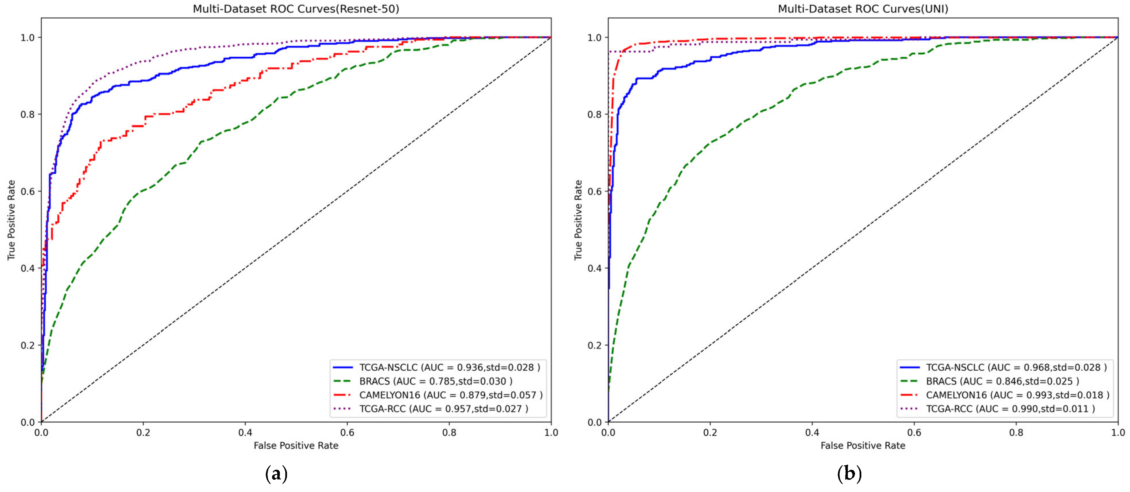
4.4. Results Analysis

Table 1 and Table 2 present the cancer diagnosis and subtype classification performance of the baseline models ResNet-50 and UNI on the TCGA-NSCLC, BRACS, CAMELYON16, and TCGA-RCC datasets. Across all four datasets, we compared our method against several representative or high-performing models proposed in recent years. The experimental results demonstrate that our model outperforms other multiple instance learning (MIL) algorithms. Specifically, when using ResNet-50 as the backbone feature extractor, our model achieved improvements of 2.3% in ACC and 2.9% in AUC over the state-of-the-art MambaMIL on the TCGA-NSCLC dataset. On the BRACS dataset, ACC and AUC improved by 2.4% and 0.7%, respectively. On the CAMELYON16 dataset, our model outperformed MambaMIL by 4.1% in ACC and 3.3% in AUC. On TCGA-RCC, our model achieved the highest ACC and AUC. Our method consistently achieves the best performance compared to all baseline methods across all datasets. Although DG-SSM-MIL uses the same aggregation and classification methods as ABMIL, our model still significantly outperforms ABMIL in both ACC and AUC. The ROC curves are shown in Figure 6a.
When using UNI as the backbone for feature extraction, the performance gap between models becomes noticeably smaller compared to using ResNet-50, which may be attributed to the more comprehensive features extracted by UNI. However, as shown in Table 2, our model still achieves strong results. On the TCGA-NSCLC and TCGA-RCC datasets, our model achieves the best performance in both ACC and AUC, with ACC values of 0.912 and 0.947 and AUC values of 0.968 and 0.990, respectively. On the BRACS and CAMELYON16 datasets, our model achieves the highest ACC and the second-best AUC, both outperforming ABMIL. This indicates that the proposed DynGraph-SSM module contributes to the improvement of classification performance to a certain extent. The ROC curves are shown in Figure 6b.

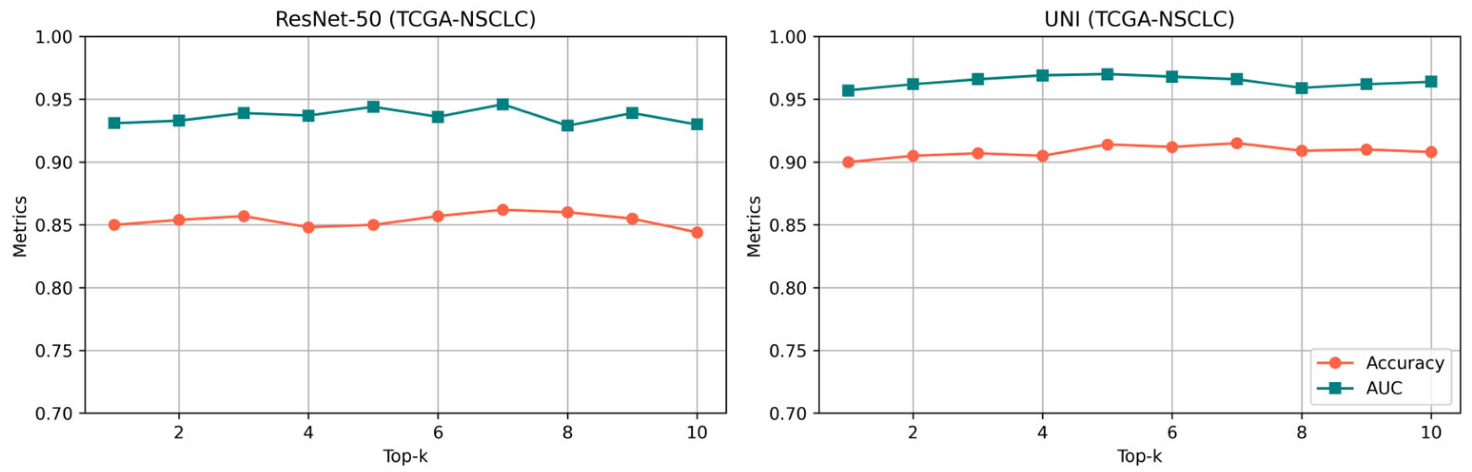
4.5. Sensitivity Analysis of the Hyperparameter

We conducted sensitivity analysis experiments on the number of neighbors k in the k-NN graph construction of the GAT path. Table 3 presents the classification ACC and AUC scores on the TCGA-NSCLC dataset when k is set to 4, 8, 12, and 16, respectively. It can be observed that the model performance fluctuates within a small range as the number of neighbors changes, indicating that the GAT path is relatively robust to the choice of k . Notably, the best performance is achieved when k = 8 , which is therefore adopted in our final model configuration.
We also conducted a sensitivity analysis on the T o p k parameter in the dynamic graph module, which controls the number of most relevant nodes selected based on attention scores. Figure 7 illustrates the variation in classification performance (ACC and AUC) on the TCGA-NSCLC dataset as the T o p k value increases from 1 to 10. The results show that the model performance remains relatively stable across different values of T o p k , demonstrating the robustness of the dynamic graph aggregation.

4.6. Ablation Study

We conducted ablation studies on two downstream tasks using the CAMELYON16 and TCGA-NSCLC datasets to evaluate the effectiveness of the proposed modules. Specifically, the CAMELYON16 dataset was used for a cancer diagnosis task, where the model determines the presence or absence of cancer, while the TCGA-NSCLC dataset was used for a cancer subtype classification task. For both tasks, the evaluation metric reported in Table 4 is the area under the ROC curve (AUC). We used the attention-based multiple instance learning framework ABMIL as the baseline model (Model A) and progressively introduced the proposed modules to assess their impact on model performance. As shown in Table 4, the abbreviations used in the results are as follows: DP—dual path; DG—dynamic graph; BS—Bi-SSM; CR—convolution refinement.
Impact of the Dual-Path Strategy. To evaluate the effectiveness of the dual-path strategy, we introduced it into Model A to create Model B. This strategy integrates the output vectors from two separate paths, one being the original feature vector and the other being the feature vector processed by GAT. These two feature vectors are used as inputs to the Mamba model to enhance feature interaction. As shown in Table 4, when using ResNet-50 as the backbone for cancer diagnosis and subtype classification, Model B achieved performance improvements of 0.8% and 1.6% over Model A, respectively. This suggests that the dual-path strategy can significantly improve performance, especially in the absence of a strong feature extractor. When using the UNI model, the performance gain was more modest, but Model B still outperformed Model A in both tasks, validating the effectiveness of the dual-path approach.
Impact of the Dynamic Graph Strategy. To assess the effectiveness of the dynamic graph (DG) strategy, we incorporated it into Model B to construct Model C. Specifically, the dual-path outputs of Model B were used as inputs to the dynamic graph, and the output of the dynamic graph was subsequently fed into the MIL module. For cancer subtype classification using ResNet-50, Model C outperformed Model B by 0.8% in both cancer diagnosis and subtyping tasks. These results suggest that integrating the dynamic graph helps enhance performance, likely due to the selective fusion of local and spatial information through the graph structure, highlighting the importance of this optimization technique in DG-SSM-MIL.
Impact of the Bi-SSM Module. We constructed Model D by feeding the output of the dynamic graph in Model C into the Bi-SSM module. When using ResNet-50 for subtype classification, Model D outperformed Model C by 0.6% in AUC. With the UNI backbone, Model D also showed improvements of 0.2% in AUC over Model C. These results indicate that the Bi-SSM module consistently outperforms the original Mamba model in classification tasks. This may be attributed to the fact that Mamba, similar to RNNs, processes sequences sequentially, whereas the Bi-SSM module mitigates this limitation by incorporating bidirectional context.
Impact of the 1D Convolution Strategy. To better adapt the model to vision tasks, we replaced the causal 1D convolution in the Bi-SSM module with standard 1D convolution. Also, we added a symmetric non-SSM path to further enhance local feature extraction. The resulting model (Model E) was compared with Model D. Although the 1D convolution strategy did not lead to a significant overall performance boost, Model E still showed consistent improvements over Model D, demonstrating its positive contribution to the final architecture.

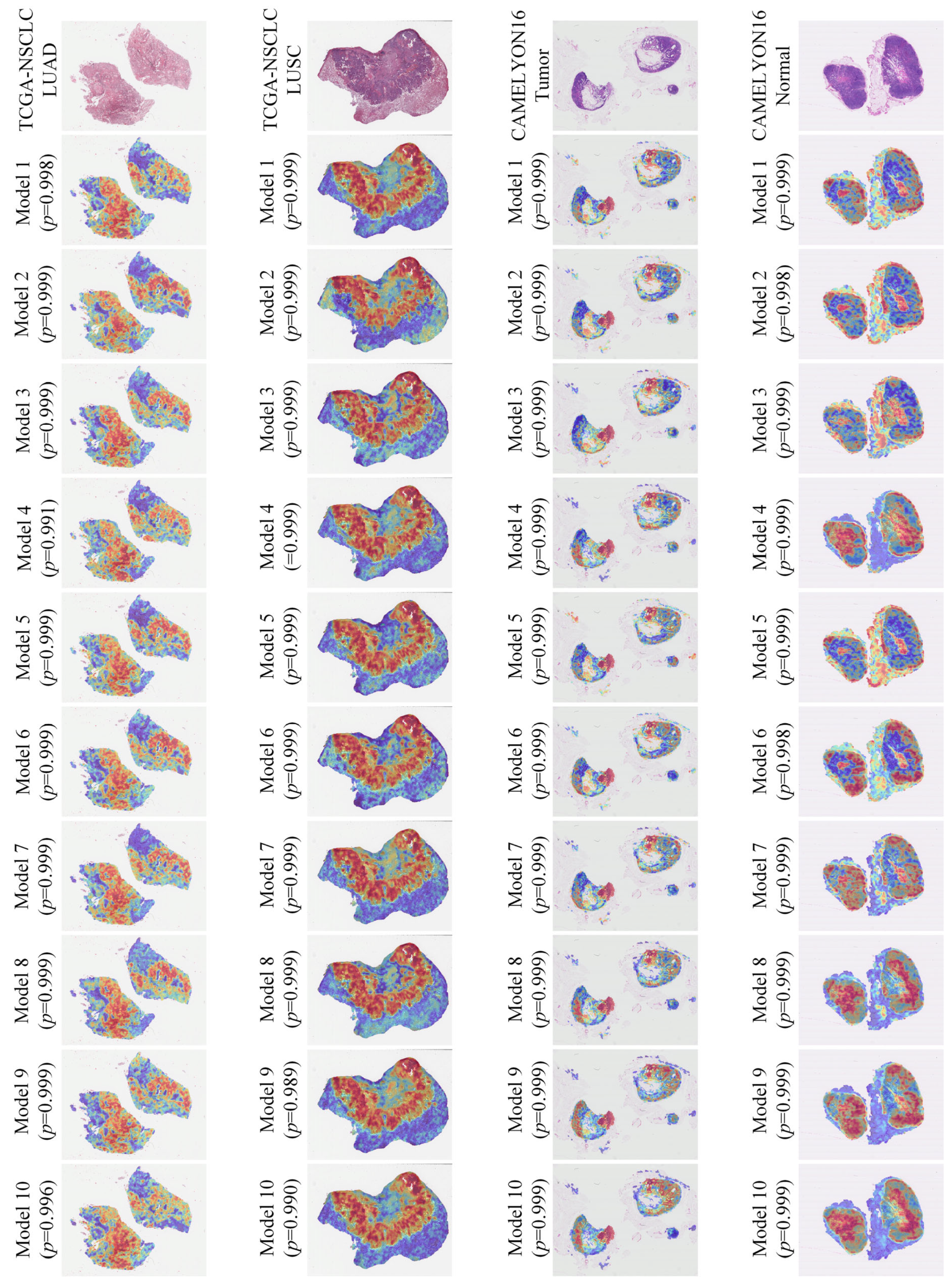
4.7. Interpretability and Attention Visualization

To illustrate the interpretability of the proposed model, we visualized the attention scores of individual patches in the WSI as heatmaps. These heatmaps highlight the most discriminative and important regions. Following the approach of Cai et al. [52], we generated attention heatmaps by converting the attention scores predicted by the model into percentiles and mapping the normalized scores back to their corresponding spatial locations in the original WSI. As shown in Figure 8, we selected the TCGA-NSCLC dataset for cancer subtype classification and CAMELYON16 for cancer detection as examples. The heatmaps shown were predicted using models obtained through 10-fold Monte Carlo cross-validation. In Figure 8, p represents the model’s confidence in making a correct prediction. It is evident that the model can accurately predict the class and localize cancer-relevant regions, demonstrating that DG-SSM-MIL offers strong interpretability and visualization capability in WSI-based cancer diagnosis and subtype classification—attributes that are of potential clinical significance.

5. Discussion

In this study, we propose an innovative multiple instance learning framework—DG-SSM-MIL—along with the design of a specialized module called DynGraph-SSM, tailored for classification tasks in whole-slide image (WSI) analysis. This module integrates a dynamic graph structure with a bidirectional state space model to effectively capture both local spatial patterns and global contextual dependencies. By combining graph neural networks and Mamba-based models, our approach achieves the effective fusion of local and global contextual information. Experimental results demonstrate that the proposed method achieves superior performance across multiple datasets, highlighting its strong capability in modeling both spatially localized features and long-range dependencies in WSI data.
This work bridges the gap between the local modeling capabilities of GNNs and the long-sequence modeling power of the Mamba architecture. Specifically, the framework introduces a dual-path strategy: one path retains the original feature vectors extracted from the image, while the other feeds spatially and locally enriched features updated by a GAT. These two feature streams are then fused through a dynamic graph, which not only integrates local and spatial information into the original sequence but also helps alleviate the challenge of dispersed tumor regions. Moreover, by constructing the dynamic graph with attention scores, the model implicitly incorporates future information, thus mitigating the limitation of Mamba’s unidirectional scanning. The updated graph features are fed into the Bi-SSM-vision module, which leverages the Mamba model’s capability for long-sequence modeling to capture global context. To better adapt to image data, we replace the 1D causal convolution in the original Mamba with a standard 1D convolution.
Experimental results on four datasets—BRACS, TCGA-NSCLC, CAMELYON16, and TCGA-RCC—demonstrate that DG-SSM-MIL outperforms most existing MIL models. By integrating a dual-path strategy, undirected and directed graph structures, and other advanced techniques, the model gains strong representational power, enabling it to effectively capture both local and global patterns in pathological data for improved classification performance.
Nevertheless, this study has certain limitations. Although attention heatmaps provide valuable insights into the regions of focus within WSIs—offering interpretability and potential assistance for clinical diagnosis—the lack of pixel-level annotations in the public datasets we used limits our ability to fully validate the model’s decision basis. Future research will involve collaboration with pathologists to obtain expert annotations on private datasets for more rigorous validation. Additionally, integrating WSI data with genomic biomarkers or clinical information holds great promise for further improving subtype classification accuracy, especially in cases with ambiguous morphological features.

6. Conclusions

The main contribution of this study lies in the effective fusion of local and global information by leveraging the complementary strengths of graph neural networks and the Mamba model. The proposed DG-SSM-MIL framework incorporates local and spatial information into feature vectors through a dynamic graph structure and utilizes attention mechanisms to address the challenge of dispersed tumor regions. Additionally, it helps mitigate the unidirectional scanning limitation of the Mamba model. The Bi-SSM-vision module is employed to extract global features from image sequences, enabling accurate and robust cancer diagnosis and subtype classification.
Experimental results on multiple datasets, including TCGA-NSCLC, BRACS, CAMELYON16, and TCGA-RCC, demonstrate that DG-SSM-MIL outperforms existing multiple instance learning models, achieving strong performance in both cancer detection and subtype classification tasks. In summary, DG-SSM-MIL offers a promising solution for WSI analysis, providing not only high classification accuracy but also good interpretability. With further optimization, this framework has the potential to become a valuable clinical tool to assist pathologists in more accurate and efficient cancer diagnosis and classification.

Author Contributions

Conceptualization, F.D. and C.C.; Data curation, F.D.; Formal analysis, F.D.; Funding acquisition, J.X.; Investigation, F.D.; Methodology, F.D. and C.C.; Software, F.D.; Supervision, Y.J. and J.X.; Validation, F.D.; Visualization, F.D.; Writing—original draft, F.D.; Writing—review and editing, C.C., J.L., M.L., and Z.W. All authors have read and agreed to the published version of the manuscript.

Funding

This work was supported by the National Key R&D Program of China (No. 2023YFC3402800), National Natural Science Foundation of China (Nos. 82441029, 62171230, 62101365, 92159301, 62301263, 62301265, 62302228, 82302291, 82302352, 62401272), Jiangsu Provincial Department of Science and Technology’s major project on frontier-leading basic research in technology (No. BK2023200).

Institutional Review Board Statement

All subjects gave their informed consent for inclusion before they participated in the study. Ethics approval is not required for this type of study. The applicable regulation can be found in Article 32 at the following link: https://www.gov.cn/zhengce/zhengceku/2023-02/28/content_5743658.htm (accessed on 2 April 2025).

Data Availability Statement

The datasets used in this study are publicly available as follows: TCGA-NSCLC and TCGA-RCC: available from The Cancer Genome Atlas (TCGA) via the Genomic Data Commons (GDC) portal: https://portal.gdc.cancer.gov (accessed on 2 April 2025). BRACS: available athttps://www.bracs.icar.cnr.it/ (accessed on 2 April 2025). CAMELYON16: available at the CAMELYON Challenge website: https://camelyon16.grand-challenge.org (accessed on 2 April 2025).

Conflicts of Interest

The authors declare no conflicts of interest.

References

  1. Cui, M.; Zhang, D.Y. Artificial intelligence and computational pathology. Lab. Investig. 2021, 101, 412–422. [Google Scholar] [CrossRef] [PubMed]
  2. Gurcan, M.N.; Boucheron, L.E.; Can, A.; Madabhushi, A.; Rajpoot, N.M.; Yener, B. Histopathological image analysis: A review. IEEE Rev. Biomed. Eng. 2009, 2, 147–171. [Google Scholar] [CrossRef]
  3. Bera, K.; Schalper, K.A.; Rimm, D.L.; Velcheti, V.; Madabhushi, A. Artificial intelligence in digital pathology—New tools for diagnosis and precision oncology. Nat. Rev. Clin. Oncol. 2019, 16, 703–715. [Google Scholar] [CrossRef] [PubMed]
  4. Li, X.; Li, C.; Rahaman, M.M.; Sun, H.; Li, X.; Wu, J.; Yao, Y.; Grzegorzek, M. A comprehensive review of computer-aided whole-slide image analysis: From datasets to feature extraction, segmentation, classification and detection approaches. Artif. Intell. Rev. 2022, 55, 4809–4878. [Google Scholar] [CrossRef]
  5. Afonso, M.; Bhawsar, P.M.; Saha, M.; Almeida, J.S.; Oliveira, A.L. Multiple Instance Learning for WSI: A comparative analysis of attention-based approaches. J. Pathol. Inform. 2024, 15, 100403. [Google Scholar] [CrossRef]
  6. Fang, Z.; Wang, Y.; Zhang, Y.; Wang, Z.; Zhang, J.; Ji, X.; Zhang, Y. Mammil: Multiple instance learning for whole slide images with state space models. In Proceedings of the 2024 IEEE International Conference on Bioinformatics and Biomedicine (BIBM), Lisboa, Portugal, 3–6 December 2024; pp. 3200–3205. [Google Scholar]
  7. Zhao, L.; Xu, X.; Hou, R.; Zhao, W.; Zhong, H.; Teng, H.; Han, Y.; Fu, X.; Sun, J.; Zhao, J. Lung cancer subtype classification using histopathological images based on weakly supervised multi-instance learning. Phys. Med. Biol. 2021, 66, 235013. [Google Scholar] [CrossRef]
  8. Zhao, W.; Guo, Z.; Fan, Y.; Jiang, Y.; Yeung, M.C.; Yu, L. Aligning knowledge concepts to whole slide images for precise histopathology image analysis. npj Digit. Med. 2024, 7, 383. [Google Scholar] [CrossRef]
  9. Ilse, M.; Tomczak, J.; Welling, M. Attention-based deep multiple instance learning. In Proceedings of the International conference on machine learning, Stockholm, Sweden, 10–15 July 2018; pp. 2127–2136. [Google Scholar]
  10. Lu, M.Y.; Williamson, D.F.; Chen, T.Y.; Chen, R.J.; Barbieri, M.; Mahmood, F. Data-efficient and weakly supervised computational pathology on whole-slide images. Nat. Biomed. Eng. 2021, 5, 555–570. [Google Scholar] [CrossRef]
  11. Zhang, H.; Meng, Y.; Zhao, Y.; Qiao, Y.; Yang, X.; Coupland, S.E.; Zheng, Y. Dtfd-mil: Double-tier feature distillation multiple instance learning for histopathology whole slide image classification. In Proceedings of the IEEE/CVF conference on computer vision and pattern recognition, New Orleans, LA, USA, 18–24 June 2022; pp. 18802–18812. [Google Scholar]
  12. Li, B.; Li, Y.; Eliceiri, K.W. Dual-stream multiple instance learning network for whole slide image classification with self-supervised contrastive learning. In Proceedings of the IEEE/CVF conference on computer vision and pattern recognition, Nashville, TN, USA, 20–25 June 2021; pp. 14318–14328. [Google Scholar]
  13. Shao, Z.; Bian, H.; Chen, Y.; Wang, Y.; Zhang, J.; Ji, X. Transmil: Transformer based correlated multiple instance learning for whole slide image classification. Adv. Neural Inf. Process. Syst. 2021, 34, 2136–2147. [Google Scholar]
  14. Chen, R.J.; Lu, M.Y.; Weng, W.-H.; Chen, T.Y.; Williamson, D.F.; Manz, T.; Shady, M.; Mahmood, F. Multimodal co-attention transformer for survival prediction in gigapixel whole slide images. In Proceedings of the IEEE/CVF international conference on computer vision, Montreal, BC, Canada, 11–17 October 2021; pp. 4015–4025. [Google Scholar]
  15. Li, H.; Yang, F.; Zhao, Y.; Xing, X.; Zhang, J.; Gao, M.; Huang, J.; Wang, L.; Yao, J. DT-MIL: Deformable transformer for multi-instance learning on histopathological image. In Proceedings of the Medical Image Computing and Computer Assisted Intervention–MICCAI 2021: 24th International Conference, Proceedings, Part VIII 24. Strasbourg, France, 27 September–1 October 2021; pp. 206–216. [Google Scholar]
  16. Vaswani, A.; Shazeer, N.; Parmar, N.; Uszkoreit, J.; Jones, L.; Gomez, A.N.; Kaiser, Ł.; Polosukhin, I. Attention is all you need. Adv. Neural Inf. Process. Syst. 2017, 30, 5998–6008. [Google Scholar]
  17. Gu, A.; Dao, T. Mamba: Linear-time sequence modeling with selective state spaces. arXiv 2023, arXiv:2312.00752. [Google Scholar]
  18. Hayat, M. Squeeze & Excitation joint with Combined Channel and Spatial Attention for Pathology Image Super-Resolution. Frankl. Open 2024, 8, 100170. [Google Scholar]
  19. Hayat, M.; Ahmad, N.; Nasir, A.; Tariq, Z.A. Hybrid Deep Learning EfficientNetV2 and Vision Transformer (EffNetV2-ViT) Model for Breast Cancer Histopathological Image Classification. IEEE Access 2024, 12, 184119–184131. [Google Scholar] [CrossRef]
  20. Zhu, L.; Liao, B.; Zhang, Q.; Wang, X.; Liu, W.; Wang, X. Vision Mamba: Efficient Visual Representation Learning with Bidirectional State Space Model. In Proceedings of the 41st International Conference on Machine Learning, Proceedings of Machine Learning Research, Vienna, Austria, 21–27 July 2024; pp. 62429–62442. [Google Scholar]
  21. Brancati, N.; Anniciello, A.M.; Pati, P.; Riccio, D.; Scognamiglio, G.; Jaume, G.; De Pietro, G.; Di Bonito, M.; Foncubierta, A.; Botti, G. Bracs: A dataset for breast carcinoma subtyping in h&e histology images. Database 2022, 2022, baac093. [Google Scholar]
  22. Ehteshami Bejnordi, B.; Veta, M.; Johannes van Diest, P.; van Ginneken, B.; Karssemeijer, N.; Litjens, G.; van der Laak, J.A.W.M.; the CAMELYON16 Consortium. Diagnostic Assessment of Deep Learning Algorithms for Detection of Lymph Node Metastases in Women With Breast Cancer. JAMA 2017, 318, 2199–2210. [Google Scholar] [CrossRef]
  23. Zhou, J.; Cui, G.; Hu, S.; Zhang, Z.; Yang, C.; Liu, Z.; Wang, L.; Li, C.; Sun, M. Graph neural networks: A review of methods and applications. AI Open 2020, 1, 57–81. [Google Scholar] [CrossRef]
  24. Wu, Z.; Pan, S.; Chen, F.; Long, G.; Zhang, C.; Philip, S.Y. A comprehensive survey on graph neural networks. IEEE Trans. Neural Netw. Learn. Syst. 2020, 32, 4–24. [Google Scholar] [CrossRef]
  25. Kipf, T.N.; Welling, M. Semi-supervised classification with graph convolutional networks. arXiv 2016, arXiv:1609.02907. [Google Scholar]
  26. Khemani, B.; Patil, S.; Kotecha, K.; Tanwar, S. A review of graph neural networks: Concepts, architectures, techniques, challenges, datasets, applications, and future directions. J. Big Data 2024, 11, 18. [Google Scholar] [CrossRef]
  27. Gilmer, J.; Schoenholz, S.S.; Riley, P.F.; Vinyals, O.; Dahl, G.E. Neural message passing for quantum chemistry. In Proceedings of the International conference on machine learning, Sydney, Australia, 6–11 August 2017; pp. 1263–1272. [Google Scholar]
  28. Veličković, P.; Cucurull, G.; Casanova, A.; Romero, A.; Lio, P.; Bengio, Y. Graph attention networks. arXiv 2017, arXiv:1710.10903. [Google Scholar]
  29. Skarding, J.; Gabrys, B.; Musial, K. Foundations and modeling of dynamic networks using dynamic graph neural networks: A survey. IEEE Access 2021, 9, 79143–79168. [Google Scholar] [CrossRef]
  30. Shi, Z.; Zhang, J.; Kong, J.; Wang, F. Integrative Graph-Transformer Framework for Histopathology Whole Slide Image Representation and Classification. In Proceedings of the International Conference on Medical Image Computing and Computer-Assisted Intervention, Marrakesh, Morocco, 6–10 October 2024; pp. 341–350. [Google Scholar]
  31. Guan, Y.; Zhang, J.; Tian, K.; Yang, S.; Dong, P.; Xiang, J.; Yang, W.; Huang, J.; Zhang, Y.; Han, X. Node-aligned graph convolutional network for whole-slide image representation and classification. In Proceedings of the IEEE/CVF Conference on Computer Vision and Pattern Recognition, New Orleans, LA, USA, 18–24 June 2022; pp. 18813–18823. [Google Scholar]
  32. Adnan, M.; Kalra, S.; Tizhoosh, H.R. Representation learning of histopathology images using graph neural networks. In Proceedings of the IEEE/CVF Conference on Computer Vision and Pattern Recognition Workshops, Seattle, WA, USA, 13–19 June 2020; pp. 988–989. [Google Scholar]
  33. Behrouz, A.; Hashemi, F. Graph mamba: Towards learning on graphs with state space models. In Proceedings of the 30th ACM SIGKDD Conference on Knowledge Discovery and Data Mining, Barcelona, Spain, 25–29 August 2024; pp. 119–130. [Google Scholar]
  34. Van der Laak, J.; Litjens, G.; Ciompi, F. Deep learning in histopathology: The path to the clinic. Nat. Med. 2021, 27, 775–784. [Google Scholar] [CrossRef] [PubMed]
  35. Deng, R.; Cui, C.; Remedios, L.W.; Bao, S.; Womick, R.M.; Chiron, S.; Li, J.; Roland, J.T.; Lau, K.S.; Liu, Q. Cross-scale multi-instance learning for pathological image diagnosis. Med. Image Anal. 2024, 94, 103124. [Google Scholar] [CrossRef] [PubMed]
  36. Chikontwe, P.; Kim, M.; Nam, S.J.; Go, H.; Park, S.H. Multiple instance learning with center embeddings for histopathology classification. In Proceedings of the Medical Image Computing and Computer Assisted Intervention–MICCAI 2020: 23rd International Conference, Lima, Peru, 4–8 October 2020; Proceedings, Part V 23, 2020. pp. 519–528. [Google Scholar]
  37. Song, A.H.; Chen, R.J.; Ding, T.; Williamson, D.F.; Jaume, G.; Mahmood, F. Morphological prototyping for unsupervised slide representation learning in computational pathology. In Proceedings of the IEEE/CVF Conference on Computer Vision and Pattern Recognition, Seattle, WA, USA, 16–22 June 2024; pp. 11566–11578. [Google Scholar]
  38. Carbonneau, M.-A.; Cheplygina, V.; Granger, E.; Gagnon, G. Multiple instance learning: A survey of problem characteristics and applications. Pattern Recognit. 2018, 77, 329–353. [Google Scholar] [CrossRef]
  39. Gu, A.; Goel, K.; Ré, C. Efficiently modeling long sequences with structured state spaces. arXiv 2021, arXiv:2111.00396. [Google Scholar]
  40. Gu, A.; Johnson, I.; Timalsina, A.; Rudra, A.; Ré, C. How to train your hippo: State space models with generalized orthogonal basis projections. arXiv 2022, arXiv:2206.12037. [Google Scholar]
  41. Li, S.; Singh, H.; Grover, A. Mamba-nd: Selective state space modeling for multi-dimensional data. In Proceedings of the European Conference on Computer Vision, Milan, Italy, 29 September–4 October 2024; pp. 75–92. [Google Scholar]
  42. Xu, R.; Yang, S.; Wang, Y.; Du, B.; Chen, H. A survey on vision mamba: Models, applications and challenges. arXiv 2024, arXiv:2404.18861. [Google Scholar]
  43. Otsu, N. A threshold selection method from gray-level histograms. Automatica 1975, 11, 23–27. [Google Scholar] [CrossRef]
  44. He, K.; Zhang, X.; Ren, S.; Sun, J. Deep residual learning for image recognition. In Proceedings of the IEEE conference on computer vision and pattern recognition, Las Vegas, NV, USA, 27–30 June 2016; pp. 770–778. [Google Scholar]
  45. Chen, R.J.; Ding, T.; Lu, M.Y.; Williamson, D.F.; Jaume, G.; Song, A.H.; Chen, B.; Zhang, A.; Shao, D.; Shaban, M. Towards a general-purpose foundation model for computational pathology. Nat. Med. 2024, 30, 850–862. [Google Scholar] [CrossRef]
  46. Ding, R.; Luong, K.-D.; Rodriguez, E.; da Silva, A.C.A.L.; Hsu, W. Combining graph neural network and mamba to capture local and global tissue spatial relationships in whole slide images. arXiv 2024, arXiv:2406.04377. [Google Scholar]
  47. Chen, R.J.; Lu, M.Y.; Shaban, M.; Chen, C.; Chen, T.Y.; Williamson, D.F.; Mahmood, F. Whole slide images are 2d point clouds: Context-aware survival prediction using patch-based graph convolutional networks. In Proceedings of the Medical Image Computing and Computer Assisted Intervention–MICCAI 2021: 24th International Conference, Proceedings, Part VIII 24. Strasbourg, France, 27 September–1 October 2021; pp. 339–349. [Google Scholar]
  48. Li, J.; Chen, Y.; Chu, H.; Sun, Q.; Guan, T.; Han, A.; He, Y. Dynamic graph representation with knowledge-aware attention for histopathology whole slide image analysis. In Proceedings of the IEEE/CVF Conference on Computer Vision and Pattern Recognition, Seattle, WA, USA, 16–22 June 2024; pp. 11323–11332. [Google Scholar]
  49. Wang, X.; He, X.; Cao, Y.; Liu, M.; Chua, T.-S. Kgat: Knowledge graph attention network for recommendation. In Proceedings of the 25th ACM SIGKDD international conference on knowledge discovery & data mining, Anchorage, AK, USA, 4–8 August 2019; pp. 950–958. [Google Scholar]
  50. Deng, J.; Dong, W.; Socher, R.; Li, L.-J.; Li, K.; Fei-Fei, L. Imagenet: A large-scale hierarchical image database. In Proceedings of the 2009 IEEE conference on computer vision and pattern recognition, Miami, FL, USA, 20–25 June 2009; pp. 248–255. [Google Scholar]
  51. Hoo, Z.H.; Candlish, J.; Teare, D. What is an ROC curve? Emerg. Med. J. 2017, 34, 357–359. [Google Scholar] [CrossRef] [PubMed]
  52. Cai, C.; Shi, Q.; Li, J.; Jiao, Y.; Xu, A.; Zhou, Y.; Wang, X.; Peng, C.; Zhang, X.; Cui, X. Pathologist-level diagnosis of ulcerative colitis inflammatory activity level using an automated histological grading method. Int. J. Med. Inform. 2024, 192, 105648. [Google Scholar] [CrossRef] [PubMed]
Figure 1. Construction of the Whole-Slide Image (WSI) Graph, where each patch is treated as a node in the graph.
Electronics 14 02056 g001
Figure 2. Overall Architecture of Dynamic Graph and State Space Model-Based MIL (DG-SSM-MIL). (a) Patch-level Feature Extraction; (b) Instance Processing Pipeline; (c) GAT-based Spatial Graph Construction; (d) Structure of the Dynamic Graph and State Space Model (DynGraph-SSM) Module.
Electronics 14 02056 g002
Figure 3. Detailed Process of Feature Fusion and Aggregation in DG-SSM-MIL.
Electronics 14 02056 g003
Figure 4. Dynamic Graph Feature Update Method. The symbol σ in the figure represents an activation function.
Electronics 14 02056 g004
Figure 5. Detailed Structure of the Bidirectional State Space Model for Vision (Bi-SSM-vision) Module.
Electronics 14 02056 g005
Figure 6. DG-SSM-MIL ROC Curves. (a) Trained on ResNet-50 features; (b) trained on UNI features.
Electronics 14 02056 g006
Figure 7. Sensitivity analysis of the Top-k parameter in the dynamic graph module.
Electronics 14 02056 g007
Figure 8. Visualization of Cancer Detection and Subtype Classification.
Electronics 14 02056 g008
Table 1. Cancer diagnosis and subtyping results (ResNet-50) on TCGA-NSCLC, BRACS, CAMELYON16, and TCGA-RCC. The best and second-best results are highlighted in bold and underline, respectively.
ModelTCGA-NSCLCBRACSCAMELYON16TCGA-RCC
AUCACCAUCACCAUCACCAUCACC
Max-Pooling0.928 ± 0.0220.841 ± 0.0290.723 ± 0.0440.411 ± 0.0430.846 ± 0.0990.793 ± 0.0810.947±0.0260.913 ± 0.026
Mean-Pooling0.907 ± 0.0290.822 ± 0.0310.727 ± 0.0380.433 ± 0.0590.795 ± 0.0980.715 ± 0.0770.940 ± 0.0210.897 ± 0.039
ABMIL0.918 ± 0.0350.838 ± 0.0450.759 ± 0.0430.435 ± 0.0570.856 ± 0.0670.811 ± 0.0540.941 ± 0.0380.906 ± 0.028
CLAM0.927 ± 0.0330.849 ± 0.0380.765 ± 0.0450.466 ± 0.0660.878 ± 0.0500.802 ± 0.0490.942 ± 0.0220.915 ± 0.032
TransMIL0.909 ± 0.0410.833 ± 0.0630.748 ± 0.0320.423 ± 0.0430.846 ± 0.0750.783 ± 0.0860.934 ± 0.0360.886 ± 0.036
S4MIL0.900 ± 0.0280.812 ± 0.0330.743 ± 0.0410.429 ± 0.0740.852 ± 0.0980.765 ± 0.0880.944 ± 0.0270.914 ± 0.023
MambaMIL0.907 ± 0.0300.834 ± 0.0340.778 ± 0.0290.456 ± 0.0730.846 ± 0.0770.790 ± 0.0600.946 ± 0.0190.927 ± 0.024
DG-SSM-MIL0.936 ± 0.0280.857 ± 0.0410.785 ± 0.0300.480 ± 0.0780.879 ± 0.0570.831 ± 0.0460.957 ± 0.0270.936 ± 0.017
Table 2. Cancer diagnosis and subtyping results (UNI) on TCGA-NSCLC, BRACS, CAMELYON16, and TCGA-RCC. The best and second-best results are highlighted in bold and underline, respectively.
ModelTCGA-NSCLCBRACSCAMELYON16TCGA-RCC
AUCACCAUCACCAUCACCAUCACC
Max-Pooling0.954 ± 0.0260.894 ± 0.0420.812 ± 0.0370.517 ± 0.0710.988 ± 0.0230.961 ± 0.0190.980 ± 0.0410.941 ± 0.013
Mean-Pooling0.957 ± 0.0240.885 ± 0.0460.809 ± 0.0310.509 ± 0.0370.912 ± 0.0660.845 ± 0.0580.979 ± 0.0230.935 ± 0.023
ABMIL0.959 ± 0.0280.899 ± 0.0390.839 ± 0.0280.544 ± 0.0430.985 ± 0.0220.970 ± 0.0310.982 ± 0.0180.931 ± 0.022
CLAM0.965 ± 0.0330.910 ± 0.0400.847 ± 0.0310.551 ± 0.0570.980 ± 0.0250.973 ± 0.0320.983 ± 0.0150.938 ± 0.018
TransMIL0.956 ± 0.0350.909 ± 0.0390.821 ± 0.0230.481 ± 0.0490.991 ± 0.0190.971 ± 0.0280.970 ± 0.0180.944 ± 0.026
S4MIL0.964 ± 0.0290.909 ± 0.0310.835 ± 0.0220.550 ± 0.0680.990 ± 0.0150.976 ± 0.0210.982 ± 0.0130.937 ± 0.014
MambaMIL0.963 ± 0.0240.901 ± 0.0360.829 ± 0.0330.537 ± 0.0590.993 ± 0.0140.975 ± 0.0170.985 ± 0.0210.942 ± 0.024
DG-SSM-MIL0.968 ± 0.0280.912 ± 0.0340.846 ± 0.0250.557 ± 0.0660.993 ± 0.0180.978 ± 0.0140.990 ± 0.0110.947 ± 0.021
Table 3. Sensitivity analysis of the number of neighbors k in k-NN graph construction on the TCGA-NSCLC dataset.
Pretrained Modelk = 4k = 8k = 12k = 16
AUCACCAUCACCAUCACCAUCACC
ResNet-500.9280.8480.9360.8570.9350.8520.9290.849
UNI0.9660.9100.9680.9120.9690.9110.9620.908
Table 4. Results of the ablation study on the CAMELYON16 and TCGA-NSCLC datasets.
ModelDesigns in DG-SSM-MILCancer DiagnosisCancer Subtyping
DPDGBSCRResNet-50UNIResNet-50UNI
A 0.8560.9850.9050.959
B 0.8640.9880.9210.963
C 0.8720.9880.9290.966
D 0.8770.9920.9350.968
E0.8790.9930.9360.968
Disclaimer/Publisher’s Note: The statements, opinions and data contained in all publications are solely those of the individual author(s) and contributor(s) and not of MDPI and/or the editor(s). MDPI and/or the editor(s) disclaim responsibility for any injury to people or property resulting from any ideas, methods, instructions or products referred to in the content.

