Research on Stochastic Dual Model Predictive Control and Application to Solar Thermal Collector Field

Abstract

Uncertainty is inevitable in real-world systems. If uncertainty is not effectively addressed, it may degrade the performance of model predictive control (MPC). This paper proposes a stochastic dual model predictive control (SDMPC) method for linear systems with parameter uncertainty and measurement noise. The method not only actively explores uncertainty while optimizing control but also introduces probabilistic output constraints to expand the set of feasible solutions. Specifically, Kalman filtering is employed to construct a real-time parameter estimator. The future output errors are incorporated into the nominal cost function as exploration signals to balance exploration and exploitation. Simulation results in the field of solar collectors show that SDMPC can effectively track the temperature by varying the inlet flow under changing environmental and opportunity constraints. The cumulative performance index of SDMPC is 125.3, compared to 316.4 obtained by conventional MPC, validating its effectiveness.

1. Introduction

Under the background of carbon neutrality, parabolic trough solar field (PTSF) systems have attracted considerable attention both domestically and internationally due to their simple structure, low cost, and high commercial maturity [1]. In practice, the solar collector field is affected by external disturbances such as solar radiation fluctuations, ambient temperature variations, and measurement noise, while internal uncertainties caused by equipment aging lead to significant parameter variations [2]. These uncertainties result in outlet temperature fluctuations, which must be mitigated by regulating the heat transfer oil flow rate. Due to the time-delay effect of the oil flow rate on the outlet temperature, inadequate prediction and control of the system dynamics may lead to temperature deviations beyond the safe operating range [3]. Therefore, the uncertainties and time-delay effect pose significant challenges to achieving stable and efficient temperature control of PTSF systems.

In recent years, model predictive control (MPC) has demonstrated excellent performance in the temperature regulation of PTSF systems [4,5]. This is largely attributed to its inherent predictive capability, which functions as an implicit feedforward mechanism and effectively addresses the issue of large thermal inertia. However, the model-based optimization process relies heavily on the accuracy of the system model [6]. The widespread uncertainties in the actual system significantly affect prediction accuracy, reducing the stability and reliability of the control. The conventional MPC often lacks proactive identification and adaptation mechanisms when dealing with unknown dynamics or parameter variations, making it difficult to achieve robust control.

To better handle system uncertainties, several advanced MPC-based strategies have been developed. When uncertainties are bounded, robust model predictive control (RMPC) ensures system robustness by considering worst-case scenarios but often leads to overly conservative control [7,8]. Its performance is heavily dependent on the accuracy of the initial model, making it unsuitable for scenarios with large disturbances or significant parameter variations. Stochastic model predictive control (SMPC) incorporates probability distributions to characterize disturbances and parameter uncertainties [9,10]. Adaptive MPC updates the system model online by identifying model parameters [11]. However, under significant uncertainty, these approaches often overlook the potential of actively exploring unknown dynamics during the control process, which may result in degraded performance. To address these limitations in highly uncertain environments, researchers have begun incorporating dual control principles into MPC to proactively learn unknown system dynamics and improve online model identification accuracy.

The dual control problem was first proposed and named by Feldbaum in 1961 [12]. He noted that applying strong excitation to a system helps reveal richer modal information, thereby enhancing the understanding of system dynamics. In contrast, mild excitation reduces overshoot and stabilizes the output more quickly. These dual effects of control signals, exploration and exploitation, are inherently conflicting [13], but their careful balance can lead to optimal control performance. The later research has shown that incorporating exploration under uncertainty can enhance control outcomes [14]. MPC excels in rolling horizon optimization, constraint handling, and real-time implementation. Dual model predictive control (DMPC) integrates exploratory mechanisms into the MPC framework. By leveraging MPC’s predictive optimization and the active learning nature of dual control, DMPC naturally embeds exploratory signals into the control process. On the one hand, cautious inputs reduce output error; on the other hand, informative inputs help probe unknown dynamics, reducing system uncertainty. DMPC provides more robust and efficient control for stochastic systems.

Early studies mainly focused on validating the feasibility and effectiveness of DMPC algorithms [15]. For instance, La proposed an online experiment design method to evaluate control performance but without experimental validation [16]. Mesbah categorized DMPC into explicit and implicit dual approaches [17]. The implicit dual methods rely on dynamic programming for numerical solutions [18], which is computationally intensive. For example, Zacekova proposed a new algorithm that achieves the dual features of model predictive control by maximizing the smallest eigenvalue of the information matrix [19]. The explicit dual control strategies introduce excitation signals explicitly to enable dual effect [20]. For instance, Houska proposed a self-reflective MPC strategy, in which the future state estimation variance is incorporated into the objective function [21]. Based on the nominal cost and an additional exploration term, Feng further optimized the weighting scheme [22]. Bujarbaruah integrated set-membership filtering to enhance robustness [23]. Heirung also incorporated the trace of the covariance estimate into the cost function [24]. However, current methods still struggle to handle parameter uncertainty effectively. In the face of many complex real-world systems [25,26], the combination of theory and practice still faces challenges.

This paper proposes a stochastic dual model predictive control (SDMPC) method for linear systems with parameter uncertainty. Kalman filtering is integrated for online parameter updates, and a prediction error term related to the estimation accuracy is inserted into the objective function. Meanwhile, the output chance constraints are considered, forming a stochastic optimal control problem. The optimal solution obtained can be carefully applied to the system while actively exploring the uncertainty of parameters. A simplified simulation model of a solar collector field temperature control system was constructed to validate the proposed SDMPC method. Simulation results demonstrate that the proposed method can actively explore parameter variations and improve control performance.

In summary, the following points encapsulate this paper’s primary contributions:

We propose an SDMPC approach that integrates active learning to reduce system uncertainty. This method alleviates the dependence of traditional MPC on model accuracy and enhances its ability to handle complex constraints by introducing probabilistic output constraints. The approach combines the dual control learning component with the constraint handling capability.

Building on a deterministic equivalent framework [24], this paper incorporates future prediction errors as exploratory signals to balance exploration and exploitation, so that the probing behavior occurs naturally. This improves parameter estimation and control performance while expanding control solutions.

We validate the proposed method through simulations on a solar collector field temperature control system. The system has the constraints of thermal oil flow rate and outlet temperature. At the same time, it has external disturbances from solar radiation, ambient temperature and measurement noise. The internal disturbances may contain parameter change caused by structural aging. The simulation shows that the SDMPC method provides robust control performance and reliable temperature tracking, proving the effectiveness of the SDMPC method.

As a result, this paper is organized as follows: The next section presents the system model and research problem. Section 3 details the proposed SDMPC approach. Section 4 models the solar collector field temperature control system and completes the simulation experiments based on the MATLAB platform. Finally, Section 5 discusses conclusions and future outlook.

2. Problem Statement

This paper considers a class of linear discrete stochastic systems.

$$\begin{array}{c}\hfill y\left(t\right)+a_{1}y(t-1)+\dots +a_{n}y(t-n)=b_{1}u(t-1)+\dots +b_{m}u(t-m)+\nu \left(t\right)\end{array}$$

(1)

where t is the discrete time and $y\left(t\right)$ and $u\left(t\right)$ represent the system output and control input, respectively. The sets ${\left\{a_i\right\}}_{i=1}^n$ and ${\left\{b_j\right\}}_{j=1}^m$ represent system parameters, with $b_1\ne 0$. Some parameters are unknown. $\nu \left(t\right)$ is additive observation noise, assumed as a Gaussian sequence with zero mean and variance r. The structure of system (1) is commonly referred to as an autoregressive model with exogenous inputs (ARX), which characterizes a linear dependency between the current output, historical outputs, and external inputs. To facilitate the explicit description of parameter uncertainty, the stochastic system can be reformulated as:

$$\begin{array}{c}\hfill y(t+1)={\theta }^T\phi \left(t\right)+\nu \left(t\right)\end{array}$$

(2)

where $y(t+1)$ is a system output measurement, determined by unknown parameter vector $\theta$, the deterministic regression vector $\phi \left(t\right)$, and the external noise $\nu \left(t\right)$. The vectors are defined as:

$$\begin{array}{cc}& \theta ={[a_1,\dots ,a_n,b_1,\dots ,b_m]}^T\\ & \phi \left(t\right)=[-y(t),\dots ,-y(t-n+1),u(t),\dots ,u(t-m+1\left)\right]\end{array}$$

Defining the information $\Psi \left(t\right)$ as the collection of all output measurements and past decisions recorded:

$$\begin{array}{c}\hfill \Psi \left(t\right)\stackrel{\Delta }{=}\{u\left(t\right),u(t-1),...,u\left(t_0\right),y\left(t\right),y(t-1),...,y\left(t_0\right)\}\end{array}$$

(3)

The finite-horizon control cost function over a prediction horizon of length N, denoted by $J_N\left(t\right)$, is defined as follows:

$$\begin{array}{c}\hfill J_N\left(t\right)\stackrel{\Delta }{=}\sum _{k=t}^{t+N-1}\left\{w_{0}E[{(y(k+1\mid t)-y^{*}(k+1\mid t))}^2\mid \Psi (k\mid t)]+w_1{u}^2(k\mid t)\right\}\end{array}$$

(4)

where N is the length of the predictive horizon. k is the sampling interval with $k=1,2,...,N-1$. At current moment t, $y(k+1\mid t)$ represents the predicted output, $u(k\mid t)$ is the input, and $y^{*}(k+1\mid t)$ is the reference trajectory. The weight values $w_0>0$ and $w_1\ge 0$ are typically chosen based on experience or empirical methods. Assuming that the past information $\Psi \left(t\right)$ is available at time t, the input sequence ${\left\{u(k\mid t)\right\}}_{k=t}^{t+N-1}$ is the problem solution, along with a sequence of control inputs for the subsequent N steps. $E\{·|\Psi (k\mid t)\}$ denotes the conditional expectation given the known information $\Psi (k\mid t)$. Note that this paper employs a finite horizon N for predictive control, and the objective function $J_N\left(t\right)$ may become unbounded in the case of an infinite horizon.

For real systems subject to constraints, input limitations are represented using simple box constraints:

$$\begin{array}{c}\hfill u_{\min }\le u(k\mid t)\le u_{\max }\end{array}$$

(5)

where $u_{min}$ and $u_{max}$ denote the lower and upper bounds of the input, respectively, typically determined by physical hardware limitations or design specifications.

For the stochastic system (2), the probabilistic characteristics of system uncertainties must be taken into account. The observation $y\left(t\right)$ also contains random qualities. Accordingly, the output chance constraint can be expressed as follows:

$$\begin{array}{c}\hfill \mathrm{Pr}[y(k+1\mid t)\ge y_{\min }|\Psi (k\mid t)]\ge 1-\alpha \end{array}$$

(6)

$$\begin{array}{c}\hfill \mathrm{Pr}[y(k+1\mid t)\le y_{\max }|\Psi (k\mid t)]\ge 1-\beta \end{array}$$

(7)

where $Pr[·|\Psi (k\mid t)]$ denotes the probability that the output satisfies the constraint, conditioned on the available information $\Psi \left(t\right)$. The $y_{min}$ and $y_{max}$ represent the lower and upper bounds of the output, respectively. Parameters $a,\beta \in (0,1]$ define the tolerable probability of violating the respective constraints.

This paper focuses on minimizing the objective function (4) for stochastic systems with parameter uncertainty and external disturbances. The output chance constraint (6), (7) and the input constraint (5) exist simultaneously. The problem is thus formulated as a stochastic optimal control problem over a finite prediction horizon N:

$$\begin{array}{}\mathrm{(8a)}& \left(\mathrm{P}\right)\hfill & \underset{u}{min}{J}_N\left(t\right)\hfill \mathrm{(8b)}& \mathrm{s}.\mathrm{t}.\hfill & y(k+1\mid t)={\theta }^T\phi (k\mid t)+\nu \left(t\right)\hfill \mathrm{(8c)}& \hfill & Pr\left[y(k+1\mid t)\ge y_{min}\mid \Psi (k\mid t)\right]\ge 1-\alpha \hfill \mathrm{(8d)}& \hfill & Pr\left[y(k+1\mid t)\le y_{max}\mid \Psi (k\mid t)\right]\ge 1-\beta \hfill \mathrm{(8e)}& \hfill & u_{min}\le u(k\mid t)\le u_{max}\hfill \mathrm{(8f)}& \hfill & k\in \{t,t+1,\dots ,t+N-1\}\hfill \end{array}$$

The constraint set (8c) and (8d) is highly nonlinear, increasing the complexity of the optimization problem. A key step in solving problem (8a) is the propagation of the mean and variance of the stochastic output $y(k+1\mid t)$ through the system dynamics in (8b). To simplify problem (8a), it is necessary to derive a deterministic propagation form of the stochastic output. Note that the inclusion of $\nu \left(t\right)$ in (8b) indicates the presence of uncertainty but does not imply the disturbed sequence is used directly for prediction.

3. Stochastic Dual Model Predictive Control

This section provides a detailed description of the proposed SDMPC algorithm. First, the evolution of parameter estimates updated at each time step is introduced. Then, the predicted output error is embedded in the objective function. Finally, the chance constraints are evaluated. The overall framework diagram of the SDMPC strategy is illustrated in Figure 1:

3.1. Parameter Estimation

For the system (2) with external noise and unknown parameters, the Kalman filter propagation form is employed for parameter estimation. Assume that the coefficients $\theta$ follow a Gaussian conditional distribution given the current information $\Psi \left(t\right)$, with mean $\widehat{\theta }\left(t\right)$ and covariance $P\left(t\right)$. The parameter estimates can be expressed as $\widehat{\theta }\left(t\right)=E[\theta \mid \Psi \left(t\right)]=[{\widehat{a}}_1\left(t\right),\dots ,{\widehat{a}}_n\left(t\right),{\widehat{b}}_1\left(t\right),\dots ,{\widehat{b}}_m\left(t\right)]$. Define the parameter estimation error as $\tilde{\theta }\left(t\right)=\theta -\widehat{\theta }\left(t\right)$ and the parameter covariance as $P\left(t\right)=\mathrm{E}\left[\tilde{\theta }\left(t\right){\tilde{\theta }}^T\left(t\right)\right|\Psi \left(t\right)]$.

Lemma 1.

For a system (2), the mean $\widehat{\theta }\left(t\right)$ and prediction conditional covariance $P\left(t\right)$ can be propagated forward as follows [27]:

$$\begin{array}{cc}& \widehat{\theta }\left(t\right)=\widehat{\theta }(t-1)+K\left(t\right){\displaystyle (}y\left(t\right)-{\widehat{\theta }}^T(t-1)\phi \left(t\right){\displaystyle )}\end{array}$$

(9)

$$\begin{array}{cc}& K\left(t\right)=P(t-1)\phi \left(t\right){\left[{\phi }^T\left(t\right)P(t-1)\phi \left(t\right)+r\right]}^{-1}\end{array}$$

(10)

$$\begin{array}{cc}& P\left(t\right)=(I-K\left(t\right){\phi }^T\left(t\right))P(t-1)\end{array}$$

(11)

where $\theta (t-1)$, $P(t-1)$, and $\phi \left(t\right)$ are given. $K\left(t\right)$ is known as the injection gain. r is the observation noise covariance.

In system (2), the regression vector $\phi (k+1\mid t)$ contains deterministic inputs and outputs, while the parameter vector $\theta \left(t\right)$ is unknown. Lemma 1 is applied to the real-time estimation of parameter $\widehat{\theta }\left(t\right)$ and its covariance $P\left(t\right)$. Therefore, a time-propagated prediction form of the output $y(k+1\mid t)$ is obtained and will be incorporated into the optimization problem as a constraint. The output conditional predictor is then defined as follows:

$$\begin{array}{c}\hfill \widehat{y}(k+1\mid t)={\widehat{\theta }}^T\left(t\right)\phi (k+1\mid t)\end{array}$$

(12)

where $\widehat{y}(k+1\mid t)$ is an estimate of the future output at the current moment t, which is used to optimize the solution of control at time $k\ge t$.

3.2. Objective Function and Constraints

The effect of estimation accuracy on controller performance is significant. Directly equating the future output $y(k+1)$ with its prediction $\widehat{y}(k+1\mid t)$ neglects the uncertainty arising from estimation errors. Worse control performance is not what we expected. To address this issue, an incentive mechanism is introduced to reward the exploratory behavior of control decisions. We define the future output variance as the errors between the true and predicted outputs:

$$\begin{array}{c}\hfill {\sigma }^2(k+1\mid t)=\mathrm{E}\left[{(y(k+1\mid t)-\widehat{y}(k+1\mid t))}^2\right|\Psi (k\mid t)]\end{array}$$

(13)

where ${\sigma }^2(k+1\mid t)$ is an incentive component term and it adds to the objective function. Unknown uncertainty can be visualized in the system output as a basis for parameter estimation at the next moment. When ${\sigma }^2(k+1\mid t)>0$, the corresponding control action actively explores uncertainty. Based on Lemma 1 and (12), define ${\sigma }^2(k+1\mid t)$ as follows:

Corollary 1.

For a system (2), given $\Psi (k\mid t)$ and $k\ge t$, the future output variance is as follows:

$$\begin{array}{c}\hfill {\sigma }^2(k+1\mid t)={\phi }^T(k+1\mid t)P(k\mid t)\phi (k+1\mid t)+r\end{array}$$

(14)

Proof of Corollary 1.

Depending on the definition of real system output, it can be derived as:

$$\begin{array}{c}\hfill \begin{array}{c}\mathrm{E}[y^2(k+1)\mid \Psi (k\mid t)]\hfill \\ =\mathrm{E}[{({\theta }^T\phi (k+1)+\nu (k+1))}^2\mid \Psi (k\mid t)]\hfill \\ =\mathrm{E}[{\left({\theta }^T\phi (k+1)\right)}^2\mid \Psi (k\mid t)]+\mathrm{E}[{\left(\nu (k+1)\right)}^2\mid \Psi (k\mid t)]\hfill \\ =\phi (k+1\mid t)\mathrm{E}[\theta {\theta }^T\mid \Psi (k\mid t)]{\phi }^T(k+1\mid t)+r\hfill \\ ={\widehat{y}}^2(k+1\mid t)+\phi (k+1\mid t)P(k\mid t){\phi }^T(k+1\mid t)+r\hfill \end{array}\end{array}$$

(15)

where the desired observation noise is $\mathrm{E}[{\left(\nu (k+1)\right)}^2\mid \Psi (k\mid t)]=r$. The parameter expectation can be expressed as $\mathrm{E}\left[\theta {\theta }^T\right|\Psi \left(k\right|t)]=P\left(k\right|t)+\widehat{\theta }\left(t\right){\widehat{\theta }}^T\left(t\right)$, which can derived from:

$$\begin{array}{c}\hfill \begin{array}{cc}\hfill P(k\mid t)& =\mathrm{E}\left[\tilde{\theta }\left(t\right){\tilde{\theta }}^T\left(t\right)\right|\Psi (k\mid t)]\hfill \\ & =\mathrm{E}\left[{(\theta -\widehat{\theta }\left(t\right))}^2\right|\Psi (k\mid t)]\hfill \\ & =\mathrm{E}\left[\theta {\theta }^T\right|\Psi (k\mid t)]-\widehat{\theta }\left(t\right){\widehat{\theta }}^T\left(t\right)\hfill \end{array}\end{array}$$

(16)

According to (13), the future output expectation error can be expressed as:

$$\begin{array}{c}\hfill \begin{array}{c}\mathrm{E}\left[{(y(k+1\mid t)-\widehat{y}(k+1\mid t))}^2\right|\Psi (k\mid t)]\hfill \\ =\mathrm{E}[y^2(k+1\mid t)\mid \Psi (k\mid t)]-{\widehat{y}}^2(k+1\mid t)\hfill \end{array}\end{array}$$

(17)

By combining (15), Corollary 1 can be directly obtained. □

Learning the uncertainty significantly reduces the prediction error. ${\sigma }^2(k+1\mid t)$ then converges to zero, and the learning process terminates automatically. Consequently, Corollary 1 enables the reformulation of $J_N\left(t\right)$, as summarized in the following theorem.

Theorem 1.

For a stochastic system (2), given $\Psi (k\mid t)$, the objective function in (4) can be written as follows:

$$\begin{array}{c}\hfill \begin{array}{cc}\hfill J_N\left(t\right)\stackrel{\Delta }{=}& \sum _{k=t}^{t+N-1}\{w_{0}E[{(\widehat{y}(k+1\mid t)-y^{*}(k+1\mid t))}^2\mid \Psi (k\mid t)]\hfill \\ & +w_1{u}^2(k\mid t)+w_2{\sigma }^2(k+1\mid t)\}\hfill \end{array}\end{array}$$

(18)

where $y^{*}(k+1\mid t))$ is the sequence of reference output. $w_0>0$, $w_1\ge 0$, and $w_2\ge 0$ are the weight coefficients.

When the ${\sigma }^2(k+1\mid t)$ shrinks to zero with the end of the study, (18) will degenerate into (4). The reward function also disappears as uncertainty dissipates.

The nonlinear constraints (8c) and (8d) in problem (8a) significantly increase the difficulty of solving the optimization problem. They are also known as opportunity constraints and are categorized as soft constraints. These can be violated under certain conditions, but the probability that the constraints hold cannot be less than a certain confidence level. This helps to expand the set of control solutions. In this paper, we consider a simplification of the nonlinear constraints with the help of Theorem 1 and Lemma 1. Typically, SDMPC uses the mean and variance information of the predicted outputs to approximate the output constraints in the actual demand. Assuming that the current information $\Phi \left(t\right)$ is known, the output measurement $y(t+1)$ follows a Gaussian distribution. The mean and variance are $\widehat{y}(k+1\mid t)={\widehat{\theta }}^T\left(t\right)\phi (k+1\mid t)$ and ${\sigma }^2(k+1\mid t)={\phi }^T(k+1\mid t)P(k\mid t)\phi (k+1\mid t)+r$. Similarly, when $k\ge t$ in the forecasting process, the future conditional distribution of $y(k+1\mid t)$ is also Gaussian. The mean $\widehat{y}(k+1\mid t)$ and variance ${\sigma }^2(k+1\mid t)$ are given in (12) and (14).

It is also proposed in [28] that the updating step of the state covariances (9) and (11) is independent of the measurements when computed using the Kalman filter. Thus, the output covariance of the prediction can be pre-calculated offline instead of online. We consider the probabilistic output constraint to have a deterministic equivalent form as follows:

$$\begin{array}{cc}& \widehat{y}(k+1\mid t)-s_{min}\sigma (k+1\mid t)\ge y_{min}\end{array}$$

(19)

$$\begin{array}{cc}& \widehat{y}(k+1\mid t)+s_{max}\sigma (k+1\mid t)\le y_{max}\end{array}$$

(20)

where $\Phi \left(s_{min}\right)=1-\alpha$ and $\Phi \left(s_{max}\right)=1-\beta$ represent the probabilities that the constraints hold. $\Phi$ denotes the standard normal cumulative distribution function (CDF). Parameters $s_{min}$ and $s_{max}$ can be determined offline in advance according to the definition of the CDF. Replacing the original constraints with these new ones during the online solution ensures that the chance constraints (8c) and (8d) are satisfied.

3.3. Stochastic Dual Model Predictive Control Algorithm

In summary, Lemma 1 provides the recursive forms of the estimates and covariances (9)–(11). Equation (12) offers the mean of the output. The future output error expectation (14) follows Corollary 1. Then, Theorem 1 defines the new cost function (18). Deterministic expressions (19) and (20) offer the output constraint chance constraints. Thus, the stochastic optimal control problem (8a) is reformulated as the problem (P^′):

$$\begin{array}{}\mathrm{(21a)}& \left({\mathrm{P}}^{\prime }\right)\hfill & \underset{u}{min}{J}_N\left(t\right)\hfill \mathrm{(21b)}& \mathrm{s}.\mathrm{t}.\hfill & \widehat{y}(k+1\mid t)={\widehat{\theta }}^T\left(t\right)\phi (k\mid t)\hfill \mathrm{(21c)}& \hfill & K(k+1\mid t)={\displaystyle \frac{P(k\mid t)\phi (k\mid t)}{{\phi }^T(k\mid t)P(k\mid t)\phi (k\mid t)+r}}\hfill \mathrm{(21d)}& \hfill & P(k+1\mid t)=\left(I-K(k\mid t){\phi }^T(k\mid t)\right)P(k\mid t)\hfill \mathrm{(21e)}& \hfill & {\sigma }^2(k+1\mid t)={\phi }^T(k+1\mid t)P(k\mid t)\phi (k+1\mid t)+r\hfill \mathrm{(21f)}& \hfill & \widehat{y}(k+1\mid t)-s_{min}\sigma (k+1\mid t)\ge y_{min}\hfill \mathrm{(21g)}& \hfill & \widehat{y}(k+1\mid t)+s_{max}\sigma (k+1\mid t)\le y_{max}\hfill \mathrm{(21h)}& \hfill & u_{min}\le u(k\mid t)\le u_{max}\hfill \mathrm{(21i)}& \hfill & k\in \{t,t+1,\dots ,t+N-1\}\hfill \end{array}$$

where $u(t-1\mid t)$, $\phi (t\mid t)$, $\widehat{\theta }\left(t\right)$, $P(t\mid t)$ given.

It is clear that the problem (P^′) is a quadratically constrained quadratic programming (QCQP) problem because of the quadratic objective function and the set of constraints. The solution ${\left\{u^0(k\mid t)\right\}}_{k=t}^{t+N-1}$ to this problem is the optimal sequence of control inputs over the N step prediction horizon. In this paper, the barrier interior point method is used as the optimization solution algorithm. The method obtains the optimal solution by traversing the interior of the feasible region, which makes it excellent in dealing with large-scale optimization problems and its feasibility preservation and computational efficiency under multi-constraints. Current research has developed many advanced nonlinear programming algorithms such as GloMIQO [29] and BARON [30]. The specific Algorithm 1 steps for SDMPC are as follows:

Algorithm 1: SDMPC

Input: the hyperstate: $\phi \left(t_0\right),u(t_0-1),\widehat{\theta }\left(t_0\right),P\left(t_0\right)$.

1: Set $t=t_0$.

2: Collecting the information $\Psi (t\mid t)$, measure $y\left(t\right)$ and $u(t-1)$.

3: Estimate parameters using Kalman filtering (9), (21c) and (21d), and update hyperstate.

4: Calculate the future estimated output $\widehat{y}(k+1\mid t)$, expectation error ${\sigma }^2(k+1\mid t)$, and chance constraints using (21b), (21e)–(21g).

5: Solve the optimization problems (P′) by using barrier interior point method, and obtain the control ${\left\{u^0(k\mid t)\right\}}_{k=t}^{t+N-1}$.

6: Apply the control $u(t\mid t)$ to the system (1).

7: Set $t=t+1$, and go back to $Step3$.

The algorithm describes the SDMPC strategies that can be used to solve (P^′). SDMPC is able to realize the control effect of output tracking in the presence of uncertainty and probabilistic output constraints of the system. In order to pursue the efficiency and reliability of simulation, this paper uses the fmincon function in the MATLAB R2023b platform to solve the problem (P^′).

4. Simulation Experiment

In order to evaluate the control performance, this paper applies the proposed SDMPC to the temperature control system of a parabolic solar collector field. A conventional MPC method and a proportional integral derivative (PID) controller are utilized for comparative analysis. Subsequently, the immunity performance of SDMPC is verified through the incorporation of simulation experiments with parameter variations and temperature setpoint changes. These uncertainties are intended to replicate the inherent variability in ambient temperature and solar radiation levels.

4.1. Modeling of Trough Solar Collector Fields

Parabolic trough solar fields (PTSFs) are spatially distributed systems that collect and store solar radiation for power generation. Precise outlet temperature control is crucial for ensuring operational safety and energy conversion efficiency. However, environmental variations introduce multiple disturbances, complicating unbiased temperature regulation. In practical PTSF operations, disturbances fall into two categories. External factors include sensor noise and weather fluctuations. Internal variations involve changes in heat transfer coefficients and the effective area of the paraboloid.

Figure 2 illustrates the system structure of a PTSF. The thermal energy collection device consists of several parallel absorber tubes and parabolic reflectors. The tube absorbs solar radiation, and the circulating oil transfers it to the heat exchanger.

Assume that the heat transfer oil flow is equally distributed. The modeling focuses on the dynamic behavior of a single tube column. According to the principle of energy conservation and the actual heat exchange process, a simulation model is constructed following [31]. The system is represented by a set of ordinary differential equations (ODEs):

$$\begin{array}{cc}& {\rho }_m{c}_m{V}_m{\displaystyle \frac{\mathrm{d}{T}_m\left(t\right)}{\mathrm{d}t}}=\eta GI\left(t\right)-h_{\mathrm{m}}{\displaystyle \frac{\pi D_{m,i}^2}{4}}\left[T_m\left(t\right)-T_f\left(t\right)\right]-h_l{\displaystyle \frac{\pi D_{m,o}^2}{4}}\left[T_m\left(t\right)-T_{\mathrm{e}}\left(t\right)\right]\end{array}$$

(22)

$$\begin{array}{cc}& {\rho }_f{c}_f{V}_f{\displaystyle \frac{\mathrm{d}{T}_o\left(t\right)}{\mathrm{d}t}}=h_m{\displaystyle \frac{\pi D_{m,i}^2}{4}}\left[T_m\left(t\right)-T_f\left(t\right)\right]+q\left(t\right){\rho }_f{c}_f\left[T_i\left(t\right)-T_o\left(t\right)\right]\end{array}$$

(23)

where (22) and (23) represent the energy balance of the heat sink and heat transfer oil, respectively. The subscripts f and m denote the heat-absorbing pipe and heat transfer oil, respectively. The outlet temperature is mainly influenced by solar radiation, ambient temperature, inlet temperature, and oil flow rate. Refer to

Table 1. Variables and parameters of PTSF system.

Parameters	Description	Value	Unit
$I\left(t\right)$	Solar radiation	/	${\mathrm{m}}^3/\mathrm{s}$
$q\left(t\right)$	Heat transfer oil flow	/	${\mathrm{m}}^3/\mathrm{s}$
$T_i\left(t\right),T_o\left(t\right)$	Inlet/outlet temperatures	/	°C
$T_e\left(t\right)$	Environmental temperature	/	°C
${\rho }_m$	Material density of collector	7850	$\mathrm{kg}/{\mathrm{m}}^3$
$c_m$	Specific collector heat capacity	460	$\mathrm{J}/(°\mathrm{C}·\mathrm{kg})$
$V_m$	Collector volume	0.01–0.02	${\mathrm{m}}^3$
${\rho }_f$	Oil mass density	780	$\mathrm{kg}/{\mathrm{m}}^3$
$c_f$	Specific oil heat capacity	1900	$\mathrm{J}/(°\mathrm{C}·\mathrm{kg})$
$V_f$	Oil volume	0.02–0.03	${\mathrm{m}}^2$
$\eta$	Optic efficiency	0.75–0.85	%
G	Effective area of concentrator	500–600	${\mathrm{m}}^2$
$D_o,D_i$	Tube O.D., I.D.	0.066, 0.070	$\mathrm{m}$
$h_m$	Heat transfer coefficient	500–600	$\mathrm{W}/({\mathrm{m}}^2·°\mathrm{C})$
$h_l$	Heat loss coefficient	5–10	$\mathrm{W}/({\mathrm{m}}^2·°\mathrm{C})$

The actual reference values are from the ACUREX field of Plataforma Solar de Almeria (PSA), located in southern Spain, and the PSA is widely used as a benchmark in solar thermal research [32].

for the specific actual parameters. The oil flow rate is a directly adjustable influence in temperature control. Assuming efficient heat transfer, $T_o\left(t\right)=T_m\left(t\right)$. Simplifying the model by capturing its key dynamic relationship with outlet temperature:

$$\begin{array}{c}\hfill \begin{array}{c}C{\displaystyle \frac{d{T}_o\left(t\right)}{dt}}=-{\displaystyle [}{h}_l{\displaystyle \frac{\pi D_{m,o}^2}{4}}+{\rho }_f{c}_{f}q\left(t\right){\displaystyle ]}{T}_o\left(t\right)+{\rho }_f{c}_f{T}_i\left(t\right)q\left(t\right)+\eta GI\left(t\right)+h_l{\displaystyle \frac{\pi D_{m,o}^2}{4}}{T}_e\left(t\right)\hfill \end{array}\end{array}$$

(24)

where $q\left(t\right)$ is the control input and $T_o\left(t\right)$ is the output value of the collector field. The physical parameter is $C={\rho }_m{c}_m{V}_m+{\rho }_f{c}_f{V}_f$.

4.2. Model Linearization

The dynamic process is assumed to be smooth and continuously differentiable. Considering the system’s nonlinearity, the model is linearized and discretized around steady-state equilibrium points, which correspond to $T_o^0=390 °\mathrm{C}$, $T_i^0=275 °\mathrm{C}$, $T_e^0=25 °\mathrm{C}$, and $I^0=851 \mathrm{W}/{\mathrm{m}}^3$, and we obtain $q^0$ by calculating $q^0={\displaystyle \frac{h_l\pi D_{m,o}^2(T_o^0-T_e^0)-\eta G{I}^o}{4{\rho }_f{c}_f(T_i^0-T_o^0)}}$. A simplified differential equation can be obtained by the linearization method in reference [33]:

$$\begin{array}{c}\hfill {\displaystyle \frac{d\Delta T_o\left(t\right)}{dt}}=a\Delta T_o\left(t\right)+b\Delta q\left(t\right)+{\mathrm{c}}_1\Delta I\left(t\right)+c_2\Delta T_i\left(t\right)+c_3\Delta T_e\left(t\right)\end{array}$$

(25)

where the sampling interval is $dt=1s$. $\Delta [·]$ denotes the deviation of the current variable from the operating point. The parameters are $a=-(h_l\pi D_{m,o}^2+4{\rho }_f{c}_f{q}^0)/4C$, $b=h_l\pi D_{m,o}^2/4C$, $c_1=\eta G/C$, $c_2={\rho }_f{c}_f{q}^0/C$, and $c_3={\rho }_f{c}_f(T_i^0-T_o^0)/C$. To clarify the proposed method’s model, Equation (25) is then rewritten in the ARX form as follows:

$$\begin{array}{c}\hfill y(t+1)=ay\left(t\right)+bu\left(t\right)+c_1{\epsilon }_1\left(t\right)+c_2{\epsilon }_2\left(t\right)+c_3{\epsilon }_3\left(t\right)+\nu \left(t\right)\end{array}$$

(26)

where the output is $y(t+1)=\Delta T_o(t+1)$ and the input is $u\left(t\right)=\Delta q\left(t\right)$, which represents the change in outlet temperature and oil flow rate, respectively. $\nu \left(t\right)$ is the observation noise, which arises from sensor inaccuracies and ambient disturbances. In control research, $\nu \left(t\right)$ is commonly modeled as Gaussian white noise due to its mathematical tractability. Let ${\epsilon }_i\left(t\right)\stackrel{\Delta }{=}\{\Delta I\left(t\right),\Delta T_i\left(t\right),\Delta T_e\left(t\right)\}$ be the external input with $i=1,2,3$, and let each follow natural laws as measurable real values. This study adopts a single-input assumption to circumvent coupling effects in multi-input systems, which can be generalized to multiple outputs. Future work will focus on decoupling methodologies to enable generalized multi-input multi-output (MIMO) implementations.

For PTSF systems, the heat transfer oil flow rate is strictly constrained within $q_{\min }\le q\le q_{\max }$, $\Delta q_{\min }\le \Delta q\le \Delta q_{\max }$. Outlet temperature constraints $T_{omin}\le T\le T_{omax}$ can be relaxed as chance constraints. This study aims to regulate the oil flow $q\left(t\right)$ to stabilize (or track) the outlet temperature $T_o\left(t\right)$ under disturbance rejection and operational constraints.

4.3. Simulation and Results

The simplified model (26) of the solar thermal collector field can be written in the form (2) mentioned in Section 3, where the $y(t+1)$ denotes the increment in outlet temperature. The known regression vector is defined as $\phi \left(t\right)=[y\left(t\right),{\epsilon }_1\left(t\right),{\epsilon }_2\left(t\right),{\epsilon }_3\left(t\right),u\left(t\right)]$. Here, ${\epsilon }_i\left(t\right)$ represents measurable but uncontrollable external inputs. $u\left(t\right)$ is the control input, denoting the change in oil flow rate. The system parameter vector ${\theta }^T=[a,c_1,c_2,c_3,b]$ is directly determined by the physical parameters listed in Table 1. Special note: since the parameter term b shows negligible variation in measurements, it is considered constant in the control-oriented model.

The prediction and control horizons are set to $N=8$ and $N_u=1$, respectively. The objective function weights are chosen as $w_0=1,w_1=0$, and $w_2={10}^{-3}$. These coefficients are chosen based on experience. The noise is set to $\nu \left(t\right)\sim \mathcal{N}(0,0.005)$. The simulation starts at $t_0=1s$ and ends at $t_f=800s$. The initial values of identification parameters are ${\widehat{\theta }}^T\left(t_0\right)=[0,0,0,0,0]$, and the covariance matrix is $P\left(t_0\right)=20\times I$, without any a priori information. The desired reference temperature is $T_{oref}=390 °\mathrm{C}$, and the initial output is $y\left(t_0\right)=-10$. The initial flow rate is set to $u\left(t_0\right)=0.0015$. The constraints are defined as $0<T_o<600$, $0<q<20$, and $-1<\Delta q<1$.

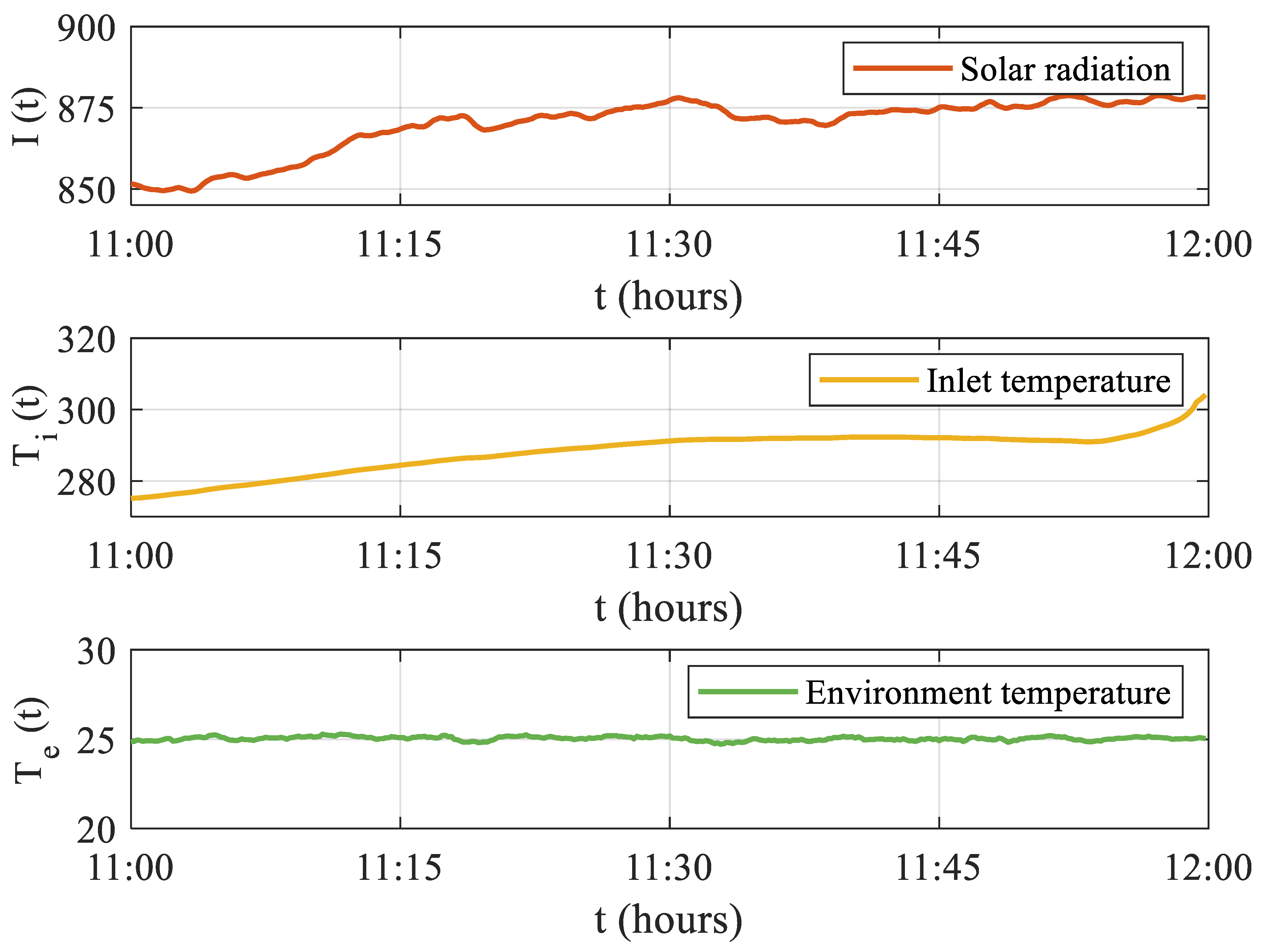
The simulation data simulate the possible variations in solar radiation, input temperature, and environment temperature from 11:00 to 12:00 noon, as shown in Figure 3. The total sampling step is $k=3600$, and we select the first 800 steps as part of the presentation.

4.3.1. Validation of Control Effectiveness

The experimental trial shows that SDMPC is able to satisfy the flow rate and output temperature constraints while stabilizing the outlet temperature.

The upper part of Figure 4 compares the outlet temperature control performance of the proposed SDMPC (blue curve), traditional MPC (red curve), and PID controller (green curve). The above three methods successfully track the reference temperature, increasing from an initial value of 380 °C to a steady-state value of 390 °C. As highlighted in the zoomed-in subplot, the SDMPC (blue curve) achieves a faster response and converges to the reference temperature (yellow curve) earlier. Meanwhile, the PID controller (green curve) exhibits more pronounced oscillations during the initial transient phase, and the baseline MPC method (red curve) shows certain oscillatory behavior. The lower part of Figure 4 shows the variation in the heat transfer oil flow rate. The control strategies show similar trends in flow rate adjustment. Comparing the results of experiments, it was demonstrated that the proposed SDMPC effectively tracks the outlet temperature and outperforms the baseline methods during the stabilization process.

In addition, the performance index comparison in Figure 5 shows that the step cost $J\left(t\right)$ of SDMPC (blue curve) remains consistently closer to zero than PID (green dashed curve) and the basic MPC (red dashed curve). The results also directly demonstrate the superior stabilization performance of the proposed SDMPC. To further validate this result, a Monte Carlo simulation was conducted. We repeated trials 500 times to obtain statistical variance, aiming to minimize randomness and enhance the reliability of the performance evaluation. The averaged performance indices are reported in

Table 2. Quantitative comparison of SDMPC, MPC, and PID.

Control Performance	SDMPC	MPC	PID
Overshoot (bandwidth 2%)	0.21823	1.9197	2.2778
Steady-state time (s)	2	2	3
Performance index	125.3124	316.4814	958.7178

. In conjunction with Figure 4 and Figure 5, it is also straightforward to conclude that the SDMPC achieves faster convergence to the desired temperature with a small overshoot, demonstrating stability and tracking capability.

4.3.2. Robustness Evaluation Under Disturbances

This subsection analyzes the dynamic response of the proposed SDMPC method under unknown perturbations. Additionally, a certain equivalent model predictive control (CEMPC) method without exploration mechanisms was implemented for comparison. It differs from SDMPC solely by disregarding the potential presence of parameter uncertainties.

In this experiment, parameter variations and outlet temperature setpoint changes are introduced. Two disturbances are applied to the system at time instances $t_c=200$ s and $t_y=400$ s, respectively. For $0<t\le t_c$, the system parameters are defined as ${\theta }^1={\left[\begin{array}{ccccc}1& 0& 0& 0& 7246.8\end{array}\right]}^T$. At $t=t_c$, the parameters abruptly switch to ${\theta }^2={\left[\begin{array}{ccccc}1.1& 0.2& 0& -0.2& 7246.8\end{array}\right]}^T$. Following this, at $t=t_y$, the outlet temperature setpoint $T_{oref}$ is adjusted from 390 to 380 °C.

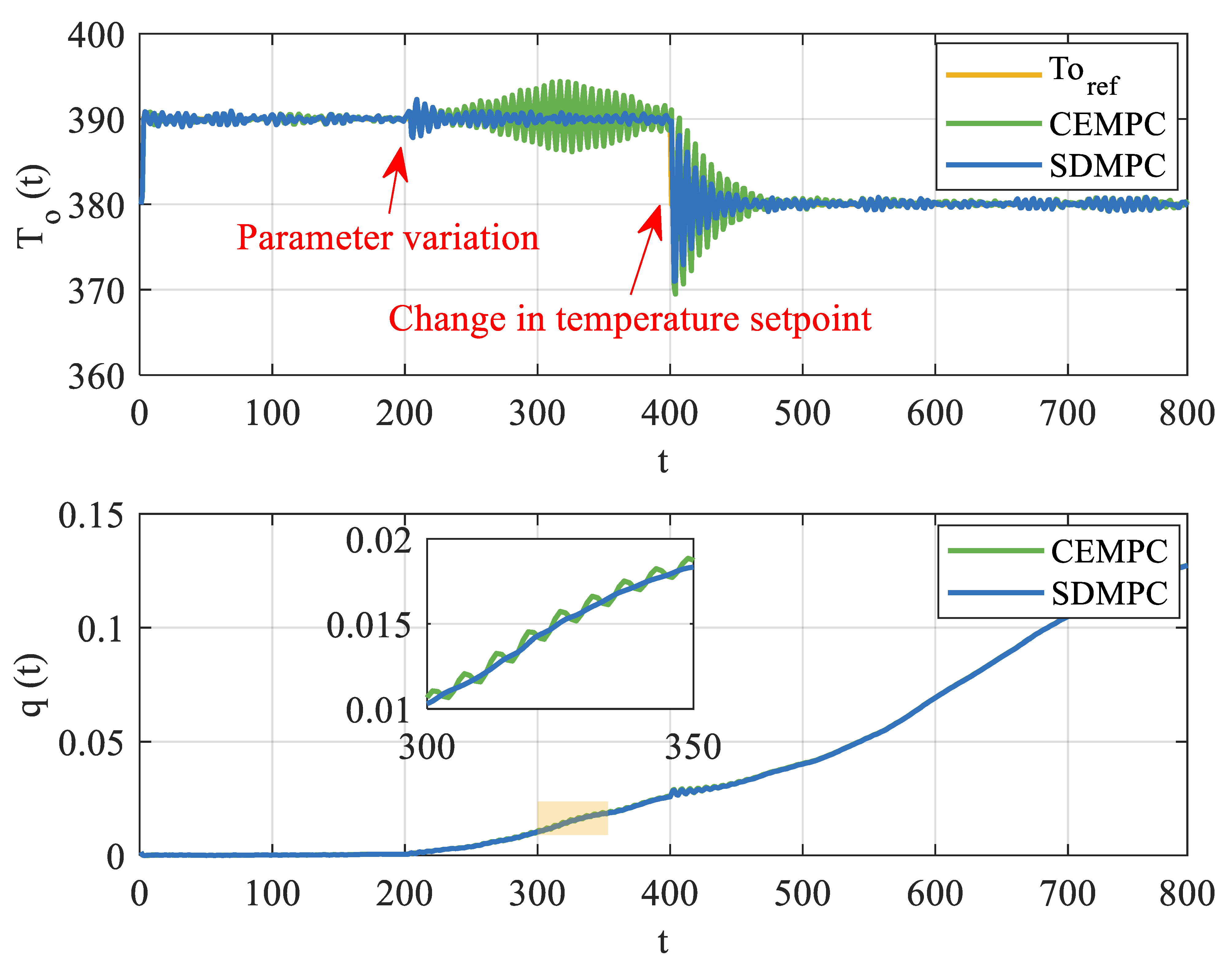
Figure 6 illustrates the system responses of two methods under both parameter variation and reference setpoint change scenarios. The red arrows highlight two key changes. The solid blue curve represents SDMPC, and the solid green curve represents CEMPC. The yellow solid line denotes the desired reference temperature. As shown in the upper part of Figure 6, sudden parameter variations at the moment t = 200 s cause fluctuation in $T_o\left(t\right)$. Compared to SDMPC, the CEMPC results in larger output deviations, primarily due to its limited capability to adapt to parameter changes. As the lower zoomed-in part, the green curve representing the flow rate, exhibits larger oscillations during the transition.Changes in the reference temperature then cause a more substantial and longer-lasting fluctuation in the tracking response. The phenomenon can be illustrated in Figure 7 and Figure 8 in detail, which show the evolution of parameter estimates and their associated covariance.

In Figure 7, the dark dashed line represents true values. The bold solid line represents SDMPC, while the lighter dashed line corresponds to CEMPC. Different colors represent different parameter elements ${\theta }_j\left(t\right)$ in turn. Taking ${\theta }_1$ (blue) as an example, at the time $t=200$ s, the SDMPC’s estimate ${\widehat{\theta }}_1\left(t\right)$ (blue solid line) quickly converges to the true value ${{\theta }_1}^2\left(t\right)=1.1$ (dark blue dashed line) via the real-time update of Kalman filter. In contrast, CEMPC’s estimate ${\widehat{\theta }}_1\left(t\right)$ (light blue line) fails to identify the true parameters even after 100 steps. When the setpoint changes at $t=400$ s, the SDMPC has acquired sufficient knowledge to allow exit temperature tracking. Also, due to the increase in output error, learning is triggered again. The yellow, green, and red curves exhibit the same characteristics.

Figure 8 illustrates the variance $P_{ii}\left(t\right)$ (the diagonal elements of $P\left(t\right)$). The upper subplot represents CEMPC, which conducts parameter learning solely at the initial time ($t=0$ s), without further adaptation thereafter. But in the lower subplot, representing SDMPC, it can be visualized that at $t=0$ s and $t=200$ s two peaks occurred. The second peak in $P_{ii}\left(t\right)$ indicates that SDMPC introduces an exploratory signal into the control inputs, accelerating the learning process of the parameters. This observation is consistent with Figure 7, illustrating the exploration and adjustment process of SDMPC under two different perturbations.

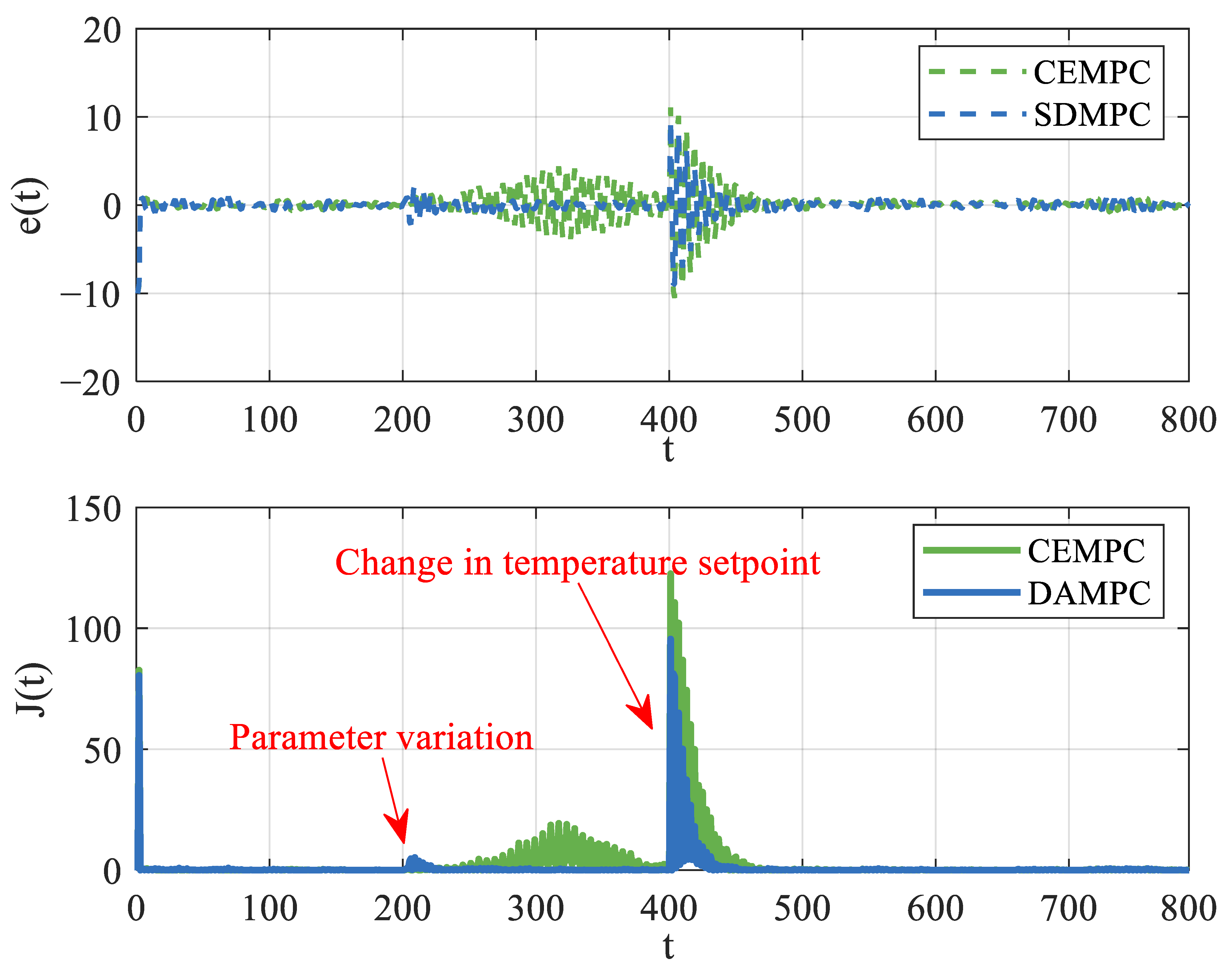
Figure 9 shows the variation in outlet temperature error $e\left(t\right)=T_o\left(t\right)-T_{oref}\left(t\right)$ and the control performance index. Both disturbances induce significant fluctuations in the output error. The error of SDMPC (blue dotted line) between 200 s and 400 s is significantly smaller than that of CEMPC (green dotted line). Correspondingly, there are two increases in control performance $J\left(t\right)$ (in the lower part of the Figure 9) observed, which is due to incorrect system parameters and large output errors. In conclusion, the SDMPC activates its exploration mechanism at the time of perturbations. SDMPC is better than CEMPC in terms of the ability to cope with parameter changes. The advantages are essential for long-term stability in solar collector control systems by mitigating parametric drift and cumulative errors.

5. Conclusions

This paper proposed a SDMPC strategy to improve MPC performance under uncertainty. By integrating stochastic dual control, the approach exploits information about system uncertainty to optimize control inputs that actively reduce its future impact. The simulation experiment is based on a solar collector field. Despite variations in solar radiation, ambient temperature, and setpoint changes, SDMPC can also accomplish output tracking tasks. The experiment results demonstrate improved parameter estimation accuracy and control performance. Future work will consider time-varying parameters to further improve the adaptivity and control quality. To take it one step further, we attempt to generalize this approach to multi-input modeling and explore its potential applications.

References

1. Islam, M.T.; Huda, N.; Abdullah, A.B. A comprehensive review of state-of-the-art concentrating solar power (CSP) technologies: Current status and research trends. Renew. Sustain. Energy Rev. 2018, 91, 987–1018. [Google Scholar] [CrossRef]
2. Su, S.; Ma, P.; Xue, Q. Optimal scheduling of extreme operating conditions in islanded microgrid based on model predictive control. Electronics 2025, 14, 206. [Google Scholar] [CrossRef]
3. Xin, X.; Zhang, Z.; Zhou, Y. A comprehensive review of predictive control strategies in heating, ventilation, and air-conditioning (HVAC): Model-free VS model. J. Build. Eng. 2024, 94, 110013. [Google Scholar] [CrossRef]
4. Pipino, H.A.; Morato, M.M.; Bernardi, E. Nonlinear temperature regulation of solar collectors with a fast adaptive polytopic LPV MPC formulation. Solar Energy 2020, 209, 214–225. [Google Scholar] [CrossRef]
5. Pataro, I.M.L.; Gil, J.D.; da Costa, M.V.A. A stochastic nonlinear predictive controller for solar collector fields under solar irradiance forecast uncertainties. IEEE Trans. Control. Syst. Technol. 2023, 32, 99–111. [Google Scholar] [CrossRef]
6. Schwenzer, M.; Ay, M.; Bergs, T. Review on model predictive control: An engineering perspective. Int. J. Adv. Manuf. Technol. 2021, 117, 1327–1349. [Google Scholar] [CrossRef]
7. Zhao, Z.; Guo, J.; Luo, X. Distributed robust model predictive control-based energy management strategy for islanded multi-microgrids considering uncertainty. IEEE Trans. Smart Grid 2022, 13, 2107–2120. [Google Scholar] [CrossRef]
8. Liang, S.; Xiao, B.; Wang, C. A Single-Tube Robust Model Predictive Control Method Based on ϵ-Approximation. Electronics 2023, 12, 2074. [Google Scholar] [CrossRef]
9. Sehr, M.A.; Bitmead, R.R. Stochastic model predictive control: Output-feedback, duality and guaranteed performance. arXiv 2017, arXiv:1706.00733. [Google Scholar]
10. Brudigam, T.; Olbrich, M.; Wollherr, D. Stochastic model predictive control with a safety guarantee for automated driving. IEEE Trans. Intell. Veh. 2021, 8, 22–36. [Google Scholar] [CrossRef]
11. Minniti, M.V.; Grandia, R.; Farshidian, F. Adaptive CLF-MPC with application to quadrupedal robots. IEEE Robot. Autom. Lett. 2021, 7, 565–572. [Google Scholar] [CrossRef]
12. Feldbaum, A.A. Dual control theory. I. Avtom. Telemekhanika 1960, 21, 1240–1249. [Google Scholar]
13. Heirung, T.A.N.; Paulson, J.A.; O’Leary, J. Stochastic model predictive control—how does it work? Comput. Chem. Eng. 2018, 114, 158–170. [Google Scholar] [CrossRef]
14. Heirung, T.A.N.; Santos, T.L.M.; Mesbah, A. Model predictive control with active learning for stochastic systems with structural model uncertainty: Online model discrimination. Comput. Chem. Eng. 2019, 128, 128–140. [Google Scholar] [CrossRef]
15. Larsson, C.A.; Rojas, C.R.; Bombois, X. Hjalmarsson, H. Experimental evaluation of model predictive control with excitation (MPC-X) on an industrial depropanizer. Process Control 2015, 31, 1–16. [Google Scholar] [CrossRef]
16. La, H.C.; Potschka, A.; Schloder, J.P. Dual control and online optimal experimental design. SIAM J. Sci. Comput. 2017, 39, 640–657. [Google Scholar] [CrossRef]
17. Mesbah, A. Stochastic model predictive control with active uncertainty learning: A survey on dual control. Annu. Rev. Control. 2018, 45, 107–117. [Google Scholar] [CrossRef]
18. Arcari, E.; Hewing, L.; Zeilinger, M.N. An approximate dynamic programming approach for dual stochastic model predictive control. IFAC-PapersOnLine 2020, 53, 8105–8111. [Google Scholar] [CrossRef]
19. Zacekova, E.; Privara, S.; Pcolka, M. Persistent excitation condition within the dual control framework. J. Process. Control. 2013, 23, 1270–1280. [Google Scholar] [CrossRef]
20. Heirung, T.A.N.; Foss, B.; Ydstie, B.E. MPC-based dual control with online experiment design. J. Process. Control. 2015, 32, 64–76. [Google Scholar] [CrossRef]
21. Houska, B.; Telen, D.; Logist, F. Self-reflective model predictive control. SIAM J. Control. Optim. 2017, 55, 2959–2980. [Google Scholar] [CrossRef]
22. Feng, X.; Houska, B. Real-time algorithm for self-reflective model predictive control. J. Process. Control. 2018, 65, 68–77. [Google Scholar] [CrossRef]
23. Bujarbaruah, M.; Zhang, X.; Tanaskovic, M. Adaptive MPC under time varying uncertainty: Robust and stochastic. arXiv 2021, arXiv:1909.1347. [Google Scholar] [CrossRef]
24. Heirung, T.A.N.; Ydstie, B.E.; Foss, B. Dual adaptive model predictive control. Automatica 2017, 80, 340–348. [Google Scholar] [CrossRef]
25. Sigounis, A.M.; Vallianos, C.; Athienitis, A. Model predictive control of air-based building integrated PV/T systems for optimal HVAC integration. Renew. Energy 2023, 212, 655–668. [Google Scholar] [CrossRef]
26. Tighirt, A.; Aatabe, M.; El Guezar, F. A new stochastic controller for efficient power extraction from small-scale wind energy conversion systems under random load consumption. Energies 2024, 17, 4927. [Google Scholar] [CrossRef]
27. Ljung, L. System identification. In Signal Analysis and Prediction; Procházka, A., Uhlíř, J., Rayner, P.W.J., Kingsbury, N.G., Benedetto, J.J., Eds.; Applied and Numerical Harmonic Analysis; Birkhäuser Boston: Boston, MA, USA, 1998; pp. 163–173. [Google Scholar]
28. Calafiore, G.C.; Dabbene, F.; Tempo, R. Research on probabilistic methods for control system design. Automatica 2011, 47, 1279–1293. [Google Scholar] [CrossRef]
29. Tawarmalani, M.; Sahinidis, N.V. Global optimization of mixed-Integer nonlinear programs: A theoretical and computational study. Math. Program. 2004, 99, 563–591. [Google Scholar] [CrossRef]
30. Misener, R.; Floudas, C.A. GloMIQO: Global mixed-integer quadratic optimizer. Glob. Optim. 2013, 57, 3–50. [Google Scholar] [CrossRef]
31. Johansen, T.A.; Storaa, C. Energy-based control of a distributed solar collector field. Automatica 2002, 38, 1191–1199. [Google Scholar] [CrossRef]
32. Gao, X.H. Optimal Model Predictive Disturbance Rejection Control Method and Application in Parabolic Trough Solar Fields. Ph.D. Thesis, Southeast University, Nanjing, China, 2022. [Google Scholar]
33. Pasamontes, M.; Álvarez, J.D.; Guzmán, J.L. A switching control strategy applied to a solar collector field. Control. Eng. Pract. 2011, 19, 135–145. [Google Scholar] [CrossRef]
Figure 1. Schematic diagram of SDMPC framework.
Electronics 14 02048 g001
Figure 2. System architecture diagram of PTSF.
Electronics 14 02048 g002
Figure 3. Evolution of collector field external measurable excitations.
Electronics 14 02048 g003
Figure 4. Control performance of outlet temperature under SDMPC, MPC, and PID.
Electronics 14 02048 g004
Figure 5. Performance index for first 50 time steps.
Electronics 14 02048 g005
Figure 6. Comparison of output temperature tracking and input trajectories under SDMPC and CEMPC.
Electronics 14 02048 g006
Figure 7. Evolution of parameter estimates θ ^ under SDMPC and CEMPC, illustrating different learning behaviors.
Electronics 14 02048 g007
Figure 8. The evolution of the diagonal elements of the covariance matrix P ( t ) over time.
Electronics 14 02048 g008
Figure 9. Output temperature tracking errors and stepwise performance indices under SDMPC and CEMPC.
Electronics 14 02048 g009