FCT: An Adaptive Model for Classification of Mixed Radio Signals

Abstract

In recent years, radio signal classification has become a hot topic in the field of wireless communication. However, current algorithms have low classification accuracy at low signal-to-noise radio (SNR) signals, and under this condition, they cannot achieve good classification results of mixed radio signals either. In this paper, we proposed an adaptive model based on feedforward neural network (FNN), convolutional neural network (CNN), and Transformer, named FCT. FCT is proposed to achieve better classification performance on mixed radio signals by leveraging the classification advantages of CNNs and Transformer networks for different SNR ratios. The parameters of FCT will be adjusted dynamically to achieve lower loss or better classification accuracy during the training process. The FCT model is verified on a public dataset, showing better performance than current state-of-the-art (SOTA) models of the mixed radio signals, especially at low SNR signals. The best classification accuracy of the FCT can reach 95.70% when the signals are at high SNR. The overall classification accuracy of FCT can reach 84.04%, which is higher than current SOTA models by 26.12%. Theoretical analysis and simulation experiments show that the proposed FCT model provides a new research direction in the classification of mixed radio signals.

1. Introduction

With time-frequency aliasing, the goal of radio signal detection is to classify the signal at a low SNR and to identify the waveform types of multiple signals present in a complex electromagnetic environment [1,2]. Experts’ prior knowledge is required for identification and spectrum judgment in traditional signal processing. With the rapid development of information, the research direction has changed from the modulation classification of a single signal to the modulation classification of multiple signals. The performance gain can be maximized by assigning signals of different energies to different users in the actual application. As a result, an effective mixed radio signal automatic modulation classification technology will have great significance.

Artificial intelligence has been widely used in image recognition, speech recognition, natural language processing, medical care, and finance in recent years. Radio signal detection can be considered as a special pattern recognition [3], and artificial intelligence can automatically extract the pattern features of radio waves, which can improve the recognition ability of radio signals in a complex electromagnetic environment compared to experience based on electromagnetic feature extraction [4].

Overall, most research into radio signals pays more attention to image-based methods [5]. Due to the advancement of neural networks in image recognition, image-based methods with salient feature images usually achieve high recognition accuracy [6]. Firstly, the radio signal is transformed into a two-dimensional picture to transform the problem of radio signal recognition into a target detection problem in the field of image classification, which can utilize the advanced achievement of artificial intelligence in the field of image recognition fully to improve the intelligent level of radio signal recognition and the recognition capability in complex electromagnetic environment.

Due to the advancement of deep learning [7,8,9,10,11], the majority of scholars have been focusing on hybrid radio classification identification in recent years, overcoming the shortcomings of traditional methods. In addition, there are still some questions about the current methods of hybrid radio classification identification. The current methods only identify signals of known mixture types. The most recent methods do not fully utilize multidimensional information and have poor identification of mixed radio signals with a low SNR ratio.

CNN models have achieved effective results in radio signal classification. Ref. [12] used real signal data to achieve a compatible recognition accuracy of modulation classification. The model of [13] was entirely a CNN, which was similar to an auto-encoder, in order to improve the modulation recognition (MR) accuracy at low SNR. Ref. [14] presented a CNN-based MR framework for the detection of radio signals in communication systems. Ref. [15], based on a deep CNN, had a higher accuracy rate for digital-signal MR at low SNR. The CLP algorithm [16] of the CNN and long short-term memory (LSTM) network in parallel was proposed to realize the fast and accurate recognition of communication signal modulation patterns, which had a good recognition effect under the condition of a low SNR ratio. The C-BiLSTM-A network, based on CNN combining with bidirectional long short-term memory (BiLSTM) and attention, had higher recognition accuracy at low SNR in [17]. Ref. [18] developed a CNN edge intelligence algorithm based on an attention mechanism to carry out the MR of the edge signal. Ref. [19] presented a D-GF-CNN algorithm based on the dilated CNN and the GF regularization function, which significantly improved recognition accuracy in the lower SNR scenarios. CCNN-Atten [20] achieved outstanding performance in dealing with radio signals with a lower sampling rate and a small signal observation window. Ref. [21] proposed a new MR method based on feature extraction to achieve a high recognition rate at low SNR. A joint conformer and CNN model [22] was proposed to separate and recognize the overlapping radio signals, which were also unknown by the monitor node, and had better performance, especially in low SNR conditions.

Transformer used stacked self-attention and point-wise, fully connected layers for both the encoder and decoder, which had powerful non-linear modeling ability to be able to better identify the characteristics of the SNR signal. The radio-image transformer [23] extracted the features from the received radio complex baseband signals, then converted the signals into images, and had good classification performance for different sampling rate signal datasets. Ref. [24] demonstrated that the Transformer can achieve higher accuracy compared to a CNN in the presence of adversarial attacks. A Transformer-based automatic classification recognition network achieved higher accuracy under low SNR ratio conditions [25].

CCNN-Atten is the most up-to-date SOTA model for processing radio signals, which is an end-to-end AMR framework [20]. However, the current algorithms have low classification accuracy at low SNR signals and cannot achieve good classification results for mixed radio signals. The L-Transformer is proposed to improve the classification accuracy at low SNR signals. On the based of the L-Transformer, the FCT algorithm is designed to solve the problem of classification of mixed radio signal. The FCT is composed of a FNN, L-CNN, and L-Transformer.

The main contributions of this paper are summarized as follows:

(1)

A Transformer-based model is proposed to improve the classification of radio signals at a low SNR.

(2)

Based on FNN, CNN, and Transformer, a new adaptive model, FCT, is proposed to achieve better classification performance on the mixed radio signals. It achieves good performance at both low SNR signals and high SNR signals.

The remainder of this paper is organized as follows. In Section 2, the mixed radio signals are described. Section 3 provides a detailed description of the L-Transformer and the FCT. Section 4 summarizes the results of the experiment, as well as a discussion of FCT and comparison models for mixed radio signals. The work is summarized in Section 5.

2. Related Work

In this section, we introduce the mixed signal model. The symbolic signal model [26] of a single signal can be written as follows:

$$r_i(n)=\sqrt{E_i}{e}^{j(2\pi f_i{T}_n+{\theta }_n)}{\sum }_{\mathcal{l}=0}^{\mathrm{L}-1}s(\mathcal{l})h(nT-\mathcal{l}T-ϵT)$$

(1)

where $i\in \left\{1,2,\dots ,\mathrm{N}\right\}$, $\sqrt{E_i}$ is the power of the signal, $s(\mathcal{l})$ is the sending symbol sequence, $h(•)$ is the channel response function, $T$ is the symbol interval, $ϵ$ is the synchronization error, $f_i$ represents the frequency offset, and ${\theta }_n$ is the phase jitter. The mixed signal is a combination of different modulation types and the mixed signal transmitter structure is shown in Figure 1.

3. Methodology

3.1. The FCT Model for Mixed Radio Signal Classification

A single type of neural network seems inefficient for dealing with mixed radio signals under different SNRs. In this section, we introduce a novel model that is based on three types of neural networks: FNN, CNN, and Transformer [27]. We call such a mixed neural network, FCT, which is shown in Figure 2.

The FCT model shown in Figure 2 is divided into six parts. The input layer consists of mixed radio signals, with data characteristics described in Section 4.1. The output results are the probability distributions for 24 types of radio signals. The core structure of the model includes one FNN, one CNN, and one Transformer network. To leverage the classification advantages of CNNs and Transformer networks for different SNR ratios, we use the FNN to perform a binary classification of radio signals based on their SNR. The results from the binary classification are then multiplied by the outputs from the CNN and Transformer, respectively. The results of these two multiplications are added together and fed into a normalization layer to perform the final classification operation.

3.2. The FNN for Recognizing SNR

The design of FNN is shown in Figure 3. FNN is used to determine whether the input signal is a high SNR signal or a low SNR signal. The output of FNN is a probability value x ranging from 0 to 1. The higher the probability x, the greater the likelihood that the input signal has an SNR above the specified threshold. If the input signal is a high SNR signal, x will be close to 1. If the signal is a low SNR signal, x will be close to 0. Here, the threshold for distinguishing between high and low SNRs is determined based on the adaptability of CNNs and Transformer networks to different SNRs. According to the experimental results, there is a clear boundary point where CNNs and Transformer networks exhibit significantly different adaptability to different SNRs, which is roughly around 0 dB. Therefore, this paper sets this threshold at 0 dB.

The FNN model is divided into four parts. The reshape layer converts the input signal represented by a three-dimensional tensor into a two-dimensional signal array without changing the data. The flatten layer does not modify the original input tensor but returns a new flattened tensor. The main purpose of the flatten operation is to facilitate the execution of the last three fully connected layer operations. The final activation layer sigmoid function outputs the probability distribution x of SNR.

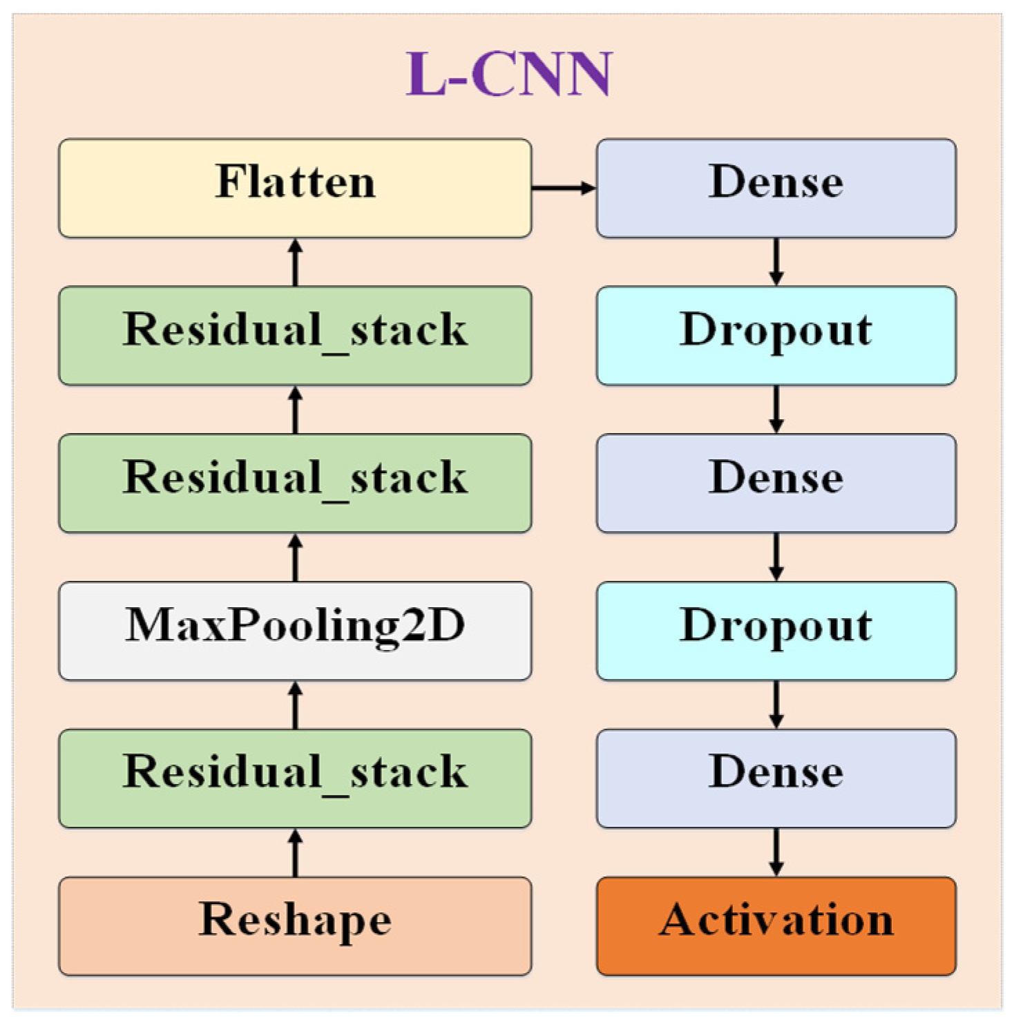
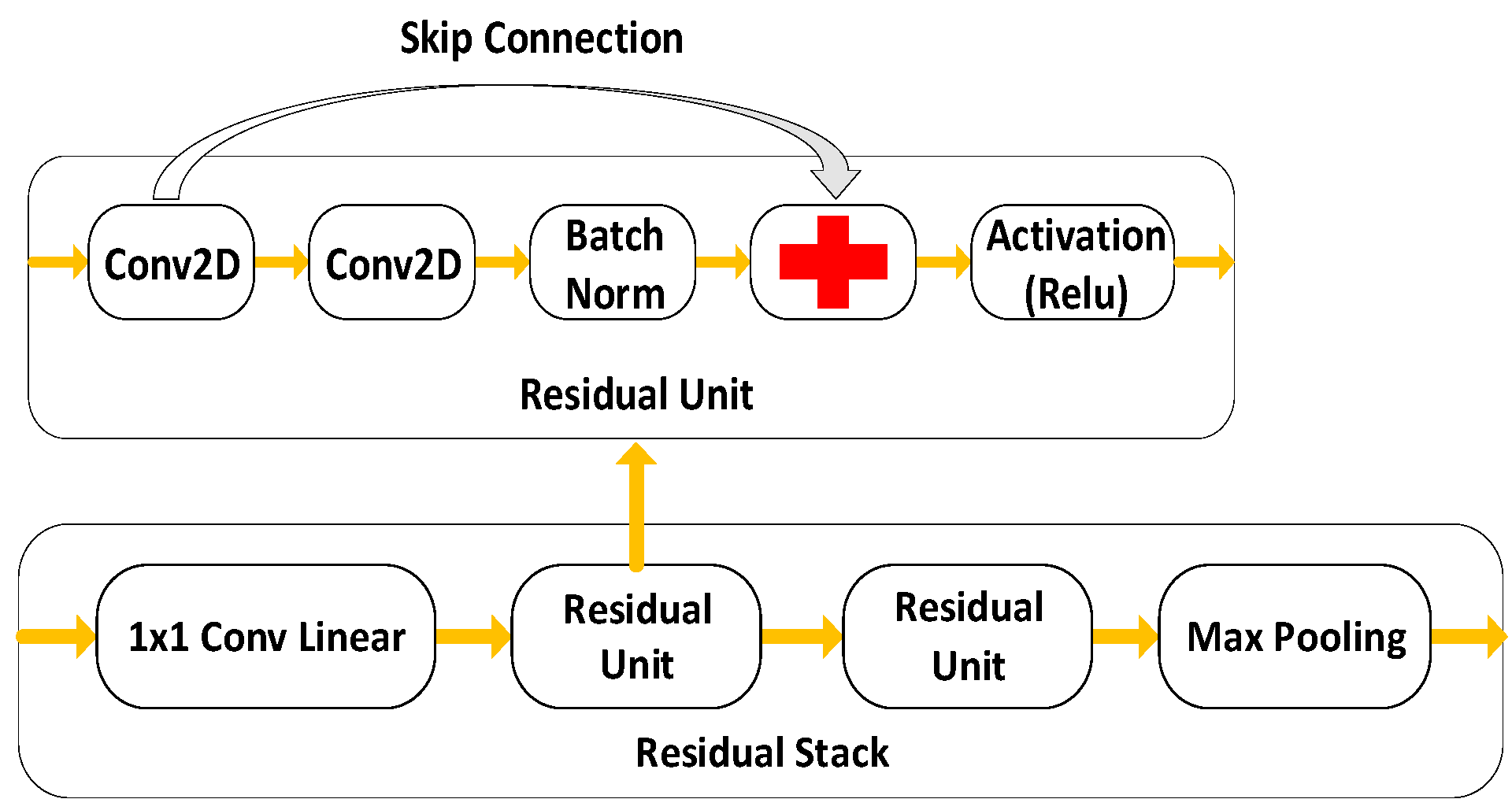
3.3. The CNN for High SNR Signal Classification (L-CNN)

The design of the L-CNN is shown in Figure 4. The L-CNN is good at identifying high SNR signals. When the mixed radio signals are sent to the L-CNN, we use x to adjust the output result of the L-CNN in the adaptive adjustment. The higher the SNR ratio, the closer x is to 1.

The L-CNN model is divided into seven parts. The reshape layer converts the input signal represented by a three-dimensional tensor into a two-dimensional signal array without changing the data. The residual stack shown in Figure 5 allows for features to operate at multiple scales and depths through the network, which reduces the need for network training. The main function of the MaxPooling2D layer is to reduce the spatial size of the input data by selecting the maximum value within a local area of the input data, while preserving important feature information of that spatial size. The flatten layer does not modify the original input tensor but returns a new flattened tensor. In the dense layer, we choose SELU activation functions to make the average of the activation vectors as close to zero as possible, accelerating the model’s convergence speed across the entire network framework, which is particularly important for signals from different SNRs. The layer of dropout is used to reduce overfitting. The final activation layer’s softmax function outputs the probability distribution x of SNR. The softmax function of the activation layer will convert the received data into a probability distribution.

$$SELU(z)=\lambda \left\{\begin{array}{cc}z& z>0\\ \alpha (exp(z)-1)& z\le 0\end{array}\right.$$

(2)

3.4. The Transformer for Low SNR Signal Classification (L-Transformer)

The design of the L-Transformer is shown in Figure 6. The L-Transformer model is divided into six parts. The reshape layer converts the input signal represented by a two-dimensional tensor into a one-dimensional signal array without changing the data. The design of a Transformer block is based on the Transformer, and the self-attention mechanism of the Transformer block can effectively identify and separate these complex features, achieving accurate classification. The GlobalAveragePooling1D layer performs average pooling on the obtained 1D array, reducing the number of parameters and computational complexity. The batch normalization layer is used to accelerate the training process of neural networks and improve the stability and performance of models. The alpha dropout layers prevent the gradient disappearance and explosion problems in self-normalized neural networks. In the dense layer, we choose SELU activation functions to accelerate the model’s convergence speed across the entire network framework, which is particularly important for signals from different SNRs.

The L-Transformer is good at identifying low SNR signals. When the mixed radio signals are sent to the L-Transformer, we use 1 − x to adjust the output result of the L-Transformer in the adaptive adjustment. The lower the SNR ratio, the closer x is to 0, the closer 1 − x is to 1, as the L-Transformer is better than the L-CNN for radio signal classification when the SNR is less than 0 dB. So, if the SNR of the signal is less than 0 dB, then the signal is a low SNR signal; otherwise, the signal is a high SNR signal.

3.5. The Training Method

During each epoch, mixed signals will be sent to the FNN, the L-CNN, and the L-Transformer. The batch size is 1024, the epochs are 1000, and the patience of the early stop mechanism is 10. Result_c is the output result of the L-CNN, and Result_t is the output result of the L-Transformer.

The calculation equation for output is shown in Equation (4), and x will be adjusted dynamically to achieve a lower loss until the optimal result that meets the conditions or the early stopping is achieved. The loss function uses categorical cross-entropy (CCE). CCE loss function performs well in multi-classification problems and can effectively measure the performance of the model. The optimizer uses Adam as it can adjust the learning rate dynamically and converge quickly. The parameters of the FNN, the L-CNN, and the L-Transformer will be adjusted during the training process.

$$\mathit{output}=x\times \mathit{Result\_c}+(1-x)\times \mathit{Result\_t}$$

(3)

$$CCE=-{\displaystyle \frac{1}{m}}{\sum }_{i=1}^m{\sum }_{j=1}^k{y}_{ij}\log \widehat{y_{ij}}$$

(4)

4. Experiments

4.1. Dataset Description

We train the FCT to the date on the subsets of DeepSig’s RadioML2018.01A [28]. The dataset has 24 modulation modes. The SNR ranges from −20 dB to 30 dB with intervals of 2 dB, for a total of 26 SNR ratios. The dataset is stored in the hdf5 file, which includes three parameters X, Y, and Z. The size of X is [1,500,000, 1024, 2]. X includes 1,500,000 signals. Each signal sample contains 1024 data points, and each data point consists of two IQ data channels. The size of Y is [1,500,000, 24]. Y corresponds to the label of each sampling point in X, which includes 1,500,000 data points and 24 modulation methods. The size of Z is [1,500,000, 1]. Z includes 1,500,000 data points and corresponds to the SNR ratio for each sampling point in X. The training and test datasets (with a ratio of 8:2) are randomly selected from each modulation type for different SNRs.

4.2. Experimental Settings

All experiments were conducted using the PyTorch 1.12 library, tensorflow-gpu 1.15, and a computer supported by NVIDIA CUDA 11.4 with a GeForce GTX 2080Ti GPU (NVIDIA, Santa Clara, CA, USA). Model training stops when the results of the test set do not improve for 10 consecutive cycles.

Two metrics, namely, the confusion matrix and the overall accuracy, are introduced to evaluate our models. Given the true positives (TP_i) for the i-th class, the accuracy is defined as follows:

$$Accuracy={\displaystyle \frac{{\sum }_{i=1}^{K}T{P}_i}{M}}$$

(5)

where K is the number of classes, and M is the number of samples in the test dataset.

The confusion matrix is used to show the performance of a classifier on various classifications, comparing the actual categories with the predicted categories to analyze the accuracy, recall, precision, and other metrics of the classification model.

4.3. Baseline Model

CCNN-Atten [20]: We chose this model for comparison, as mentioned in the Introduction. CCNN-Atten algorithms are the up-to-date SOTA models for processing radio signals, which use a deep-learning-based end-to-end framework named CCNN-Atten to improve the AMR accuracy of raw complex-valued signals at low computational complexity. This algorithm relies on two modules, complex-valued CNN and feature calibration, to extract features from the communication baseband signal.

Ti-CNN [28]: Ti-CNN comprises a number of convolutional layers followed by fully connected layers (FC) in classifiers. The filter size is minimized at 3 × 3, and the smallest size pooling operations are used at 2 × 2. We used these variables to reference the Ti-CNN, but the parameters were trained by ourselves.

4.4. Comparison with Baseline Method

We compare the L-Transformer with the baseline algorithm on the RadioML2018.01A datasets to verify the effectiveness of the proposed method.

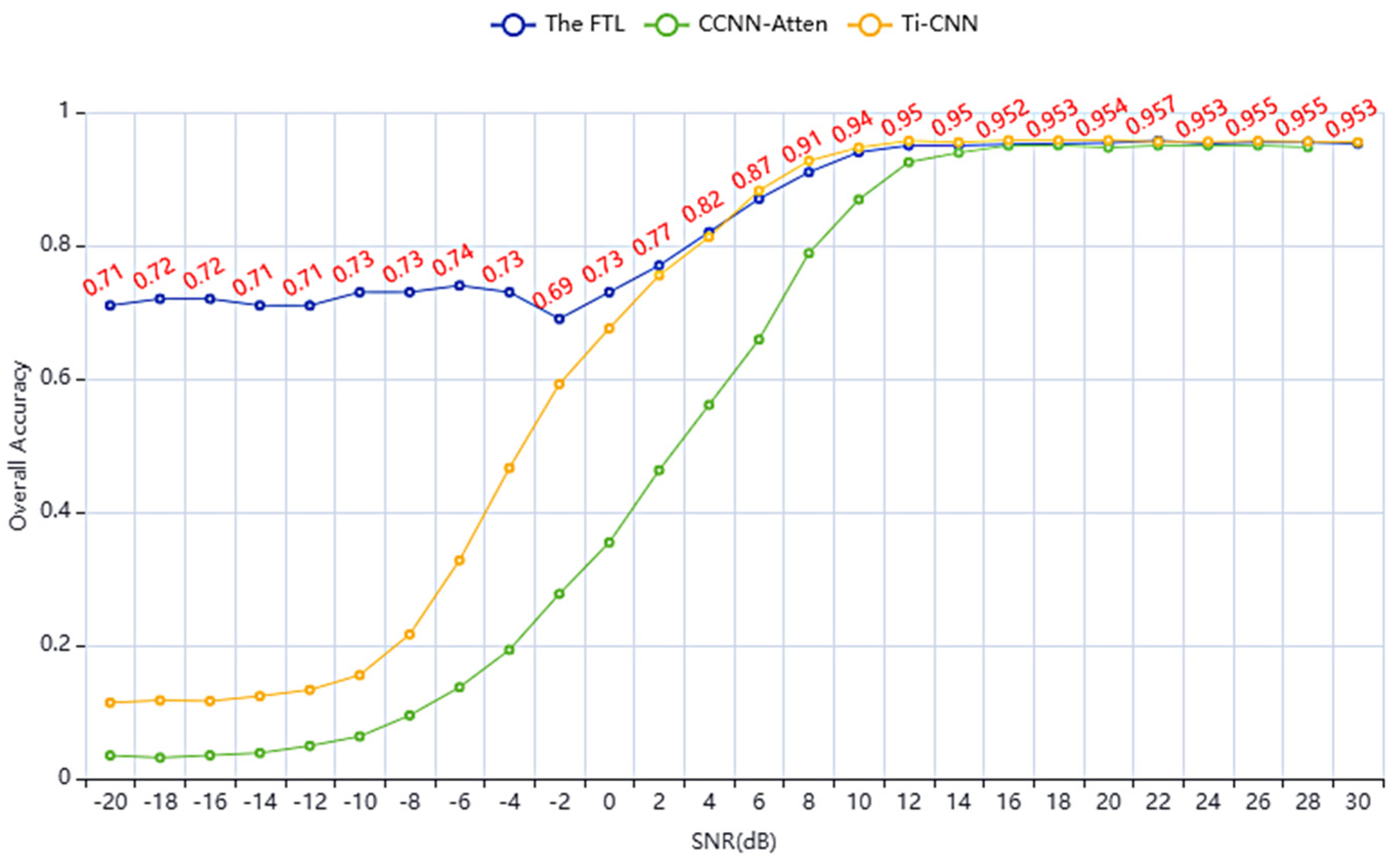
4.4.1. The Result of Classification Accuracy

Figure 7 shows the mixed radio signal classification accuracy of the L-Transformer and the Ti-CNN. As can be seen, the performance of the L-Transformer is better than the Ti-CNN for classification when the SNR is less than 0 dB, and the performance of the Ti-CNN is better than the L-Transformer for classification when the SNR is higher than 0 dB. And 0 dB is truly the optimal cutoff point between high and low SNR signals.

Figure 8 shows the mixed radio signals classification accuracy of the FCT, the CCNN-Atten, and the Ti-CNN under different SNRs. The performance of the FCT and the Ti-CNN is almost the same at high SNR signals, while the CCNN-Atten performs slightly worse. The best classification accuracy of the FCT can reach 95.70%. In addition, the FCT performs better than the CCNN-Atten and the Ti-CNN at low SNR, as shown in Figure 8.

Table 1. Comparison of the classification accuracy of the three models. The dataset is RadioML2018.01A.

Model	Ti-CNN	CCNN-Atten	FCT
Accuracy	65.11%	57.92%	84.04%

shows the overall classification accuracy. The overall classification accuracy of the FCT is 84.04%, and the overall classification accuracy of the CCNN-Atten and the Ti-CNN are 57.92% and 65.11%. The overall classification accuracy of the FCT is higher than the CCNN-Atten by 26.12% and is higher than the Ti-CNN by 18.93%.

4.4.2. The Result of the Confusion Matrix

In Figure 9, we show a confusion matrix result of the Ti-CNN algorithm for the classifier across all 24 classes. In Figure 10, we show a confusion matrix result of the FCT algorithm for the classifier across all 24 classes. A confusion matrix result of the CCNN-Atten algorithm for the classifier across all 24 classes is shown in [20]. The confusion matrix diagonal is clearer as the SNR increases, indicating that the classification accuracy increases as the SNR increases. We can reach the conclusion that the FCT algorithm achieves the best classification results for mixed radio signals. In other words, the FCT performs better than the Ti-CNN and the CCNN-Atten for the classification of the mixed radio signals.

5. Conclusions

In this paper, we propose the L-Transformer to improve the classification of radio signals at low SNRs. Then, on the basis of the FNN, the L-CNN, and the L-Transformer, the FCT algorithm is proposed to reach better classification results of the mixed radio signals. The FCT algorithm is an adaptive adjustment model, and the parameters of the FCT algorithm will be adjusted to achieve lower loss or better classification accuracy during the training process. The FCT algorithm is verified on the RadioML2018.01A dataset. The experiments show that the FCT is better than the CCNN-Atten and the Ti-CNN for the classification of the mixed radio signals. The best classification accuracy of the FCT can reach 95.70%. The overall classification accuracy of the FCT can reach 84.04%. The FCT algorithm provides a new idea about the classification of mixed radio signal modulation. The mixed signal recognition problem can easily become a data fitting problem without actual tests, and the size and quality of the synthetic dataset may not cover all possibilities of real-world scenarios. In our future work, we will explore the FCT algorithm’s performance in real-acquired modulated signal datasets, such as USRP tests.

References

1. Xie, X.; Yang, G.; Jiang, M.; Ye, Q.; Yang, C.-F. A Kind of Wireless Modulation Recognition Method Based on DenseNet and BLSTM. IEEE Access 2021, 9, 125706–125713. [Google Scholar] [CrossRef]
2. Liu, D.; Ergun, K.; Rosing, T.Š. Towards a Robust and Efficient Classifier for Real World Radio Signal Modulation Classification. In Proceedings of the ICASSP 2023—2023 IEEE International Conference on Acoustics, Speech and Signal Processing (ICASSP), Rhodes Island, Greece, 4–10 June 2023; pp. 1–5. [Google Scholar] [CrossRef]
3. Luo, R.; Hu, T.; Tang, Z.; Wang, C.; Gong, X.; Tu, H. A Radio Signal Modulation Recognition Algorithm Based on Residual Networks and Attention Mechanisms. arXiv 2019, arXiv:1909.12472. [Google Scholar]
4. Fonseca, E.; Santos, J.; Paisana, F.; DaSilva, L.A. Radio Access Technology Characterisation Through Object Detection; Elsevier: Amsterdam, The Netherlands, 2021. [Google Scholar] [CrossRef]
5. Konan, O.J.E.Y.; Mishra, A.K.; Lotz, S. Machine Learning Techniques to Detect and Characterise Whistler Radio Waves. arXiv 2020, arXiv:2002.01244. [Google Scholar]
6. Xu, J.; Wu, C.; Ying, S.; Li, H. The Performance Analysis of Complex-Valued Neural Network in Radio Signal Recognition. IEEE Access 2022, 10, 48708–48718. [Google Scholar] [CrossRef]
7. Xiao, W.; Luo, Z.; Hu, Q. A Review of Research on Signal Modulation Recognition Based on Deep Learning. Electronics 2022, 11, 2764. [Google Scholar] [CrossRef]
8. Wang, T.; Yang, G.; Chen, P.; Xu, Z.; Jiang, M.; Ye, Q. A Survey of Applications of Deep Learning in Radio Signal Modulation Recognition. Appl. Sci. 2022, 12, 12052. [Google Scholar] [CrossRef]
9. Li, X.; Dong, F.; Zhang, S.; Guo, W. A Survey on Deep Learning Techniques in Wireless Signal Recognition. Wirel. Commun. Mob. Comput. 2019, 2019, 5629572. [Google Scholar] [CrossRef]
10. Elyousseph, H.; Altamimi, M.L. Deep Learning Radio Frequency Signal Classification with Hybrid Images. In Proceedings of the 2021 IEEE International Conference on Signal and Image Processing Applications (ICSIPA), Kuala Terengganu, Malaysia, 13–15 September 2021; pp. 7–11. [Google Scholar]
11. Wang, F.; Zhou, Y.; Yan, H.; Luo, R. Enhancing the generalization ability of deep learning model for radio signal modulation recognition. Appl. Intell. 2023, 53, 18758–18774. [Google Scholar] [CrossRef]
12. Xu, Y.; Li, D.; Wang, Z.; Guo, Q.; Xiang, W. A deep learning method based on convolutional neural network for automatic modulation classification of wireless signals. Wireless Netw. 2019, 25, 3735–3746. [Google Scholar] [CrossRef]
13. Liu, Y.; Liu, Y. Modulation recognition with pre-denoising convolutional neural network. Electron. Lett. 2019, 56, 3586. [Google Scholar] [CrossRef]
14. Zeng, Y.; Zhang, M.; Han, F.; Gong, Y.; Zhang, J. Spectrum Analysis and Convolutional Neural Network for Automatic Modulation Recognition. IEEE Wirel. Commun. Lett. 2019, 8, 929–932. [Google Scholar] [CrossRef]
15. Jiang, K.; Zhang, J.; Wu, H.; Wang, A.; Iwahori, Y. A Novel Digital Modulation Recognition Algorithm Based on Deep Convolutional Neural Network. Appl. Sci. 2020, 10, 1166. [Google Scholar] [CrossRef]
16. Huang, Z.; Li, C.; Lv, Q.; Su, R.; Zhou, K. Automatic Recognition of Communication Signal Modulation Based on the Multiple-Parallel Complex Convolutional Neural Network. Wirel. Commun. Mob. Comput. 2021, 2021, 5006248. [Google Scholar] [CrossRef]
17. Jiang, K.; Qin, X.; Zhang, J.; Wang, A. Modulation Recognition of Communication Signal Based on Convolutional Neural Network. Symmetry 2021, 13, 2302. [Google Scholar] [CrossRef]
18. Jiao, J.; Sun, X.; Zhang, Y.; Liu, L.; Shao, J.; Lyu, J.; Fang, L. Modulation Recognition of Radio Signals Based on Edge Computing and Convolutional Neural Network. J. Commun. Inf. Netw. 2021, 6, 280–300. [Google Scholar] [CrossRef]
19. Du, R.; Liu, F.; Xu, J.; Gao, F.; Hu, Z.; Zhang, A. D-GF-CNN Algorithm for Modulation Recognition. Wireless Pers. Commun. 2022, 124, 989–1010. [Google Scholar] [CrossRef]
20. Liang, Z.; Tao, M.; Xie, J.; Yang, X.; Wang, L. A Radio Signal Recognition Approach Based on Complex-Valued CNN and Self-Attention Mechanism. IEEE Trans. Cogn. Commun. Netw. 2022, 8, 1358–1373. [Google Scholar] [CrossRef]
21. Liang, J.; Li, X.; Liang, C.; Tong, H.; Mai, X.; Kong, R. JCCM: Joint conformer and CNN model for overlapping radio signals recognition. Electron. Lett. 2023, 59, 13006. [Google Scholar] [CrossRef]
22. Liu, F.; Zhang, Z.; Zhou, R. Automatic modulation recognition based on CNN and GRU. Tsinghua Sci. Technol. 2022, 27, 422–431. [Google Scholar] [CrossRef]
23. Chen, S.; Qiu, K.; Zheng, S.; Xuan, Q.; Yang, X. Radio-Image:Bridging Radio Modulation Classification and ImageNet Classification. Electronics 2020, 9, 1646. [Google Scholar] [CrossRef]
24. Zhang, L.; Lambotharan, S.; Zheng, G. Adversarial Learning in Transformer Based Neural Network in Radio Signal Classification. In Proceedings of the ICASSP 2022—2022 IEEE International Conference on Acoustics, Speech and Signal Processing (ICASSP), Singapore, 22–27 May 2022; pp. 9032–9036. [Google Scholar] [CrossRef]
25. Zheng, Y.; Ma, Y.; Tian, C. TMRN-GLU: A Transformer-Based Automatic Classification Recognition Network Improved by Gate Linear Unit. Electronics 2022, 11, 1554. [Google Scholar] [CrossRef]
26. Xu, J.; Lin, Z. Modulation and Classification of Mixed Signals Based on Deep Learning. arXiv 2022, arXiv:2205.09916. [Google Scholar]
27. Vaswani, A.; Shazeer, N.; Parmar, N.; Uszkoreit, J.; Jones, L.; Gomez, A.N.; Kaiser, Ł.; Polosukhin, I. Attention is all you need. In Proceedings of the 31st International Conference on Neural Information Processing Systems (NIPS’17), Long Beach, CA, USA, 4–9 December 2017; Curran Associates Inc.: Red Hook, NY, USA, 2017; pp. 6000–6010. [Google Scholar]
28. O’Shea, T.J.; Roy, T.; Clancy, T.C. Over-the-Air Deep Learning Based Radio Signal Classification. IEEE J. Sel. Top. Signal Process. 2018, 12, 168–179. [Google Scholar] [CrossRef]
Figure 1. Mixed signal transmitter structure.
Electronics 14 02028 g001
Figure 2. The structure of the FCT.
Electronics 14 02028 g002
Figure 3. The structure of the FNN.
Electronics 14 02028 g003
Figure 4. The structure of the L-CNN.
Electronics 14 02028 g004
Figure 5. Residual unit and residual stack.
Electronics 14 02028 g005
Figure 6. The structure of the L-Transformer.
Electronics 14 02028 g006
Figure 7. The comparison results of L-Transformer and Ti-CNN.
Electronics 14 02028 g007
Figure 8. Mixed radio signal classification overall accuracy using FCT.
Electronics 14 02028 g008
Figure 9. Ti-CNN confusion matrix result for mixed radio signals.
Electronics 14 02028 g009
Figure 10. The FCT confusion matrix for mixed radio signals.
Electronics 14 02028 g010