Energy Efficiency Optimization of Multi-Hop Relay Networks via a Joint Relay Selection and Power Allocation Strategy

Abstract

Existing resource allocation models for multi-hop relay networks lack the systematic joint optimization of relay selection and power allocation. Therefore, a multi-hop relay network model based on a joint optimization strategy is proposed, aimed at realizing the energy efficiency optimization of the system through the cooperative optimization of relay selection and power allocation. The proposed model not only takes into account the node transmitting power and communication link but also combines the specified system quality of service requirements. On this basis, the FD-Dink energy efficiency optimization algorithm is proposed. By integrating an enhanced D* algorithm with a forward maximum signal-to-noise ratio (FMSNR) and the Dinkelbach–Lagrange multiplier method, the proposed strategy resolves relay selection and power control problems in a coordinated framework so as to determine the optimal energy efficiency communication link of a multi-hop relay network model. Case studies demonstrate that this joint optimization strategy significantly improves the system energy efficiency of the multi-hop relay network and shows superiority in dynamic path planning and global power allocation, offering significant theoretical and practical implications.

1. Introduction

With the advancement of smart grid systems toward digitalization and intelligence, the performance demands on wireless private power networks—serving as critical infrastructure for real-time monitoring, precise control, and high-volume data transmission—are becoming increasingly stringent [1,2]. However, wireless private power networks often face challenges, including the widespread distribution of nodes and complex environmental conditions. Consequently, traditional single-hop communication technology struggles to satisfy the demands for extensive coverage and highly reliable transmission. By flexibly deploying relay nodes, multi-hop relay technology has emerged as one of the crucial solutions for power wireless private networks. This technology can effectively expand network coverage and enhance transmission stability [3,4].

Despite advancements in relay selection and power allocation, several critical challenges remain unresolved [5,6,7,8,9,10,11,12]. Firstly, the power wireless private network is characterized by high node density, limited coverage, and strict QoS requirements. Nevertheless, the majority of existing algorithms concentrate on general scenarios or particular hops, without adequately addressing the unique characteristics of node density and limited coverage inherent in power scenarios. For instance, reference [12] presents a dynamic selection algorithm that integrates spatial position and channel state analysis. However, its applicability is confined to two-hop situations, rendering it less adaptable to multi-hop networks. Similarly, reference [13] enhances path planning by refining the A* algorithm, yet it fails to account for the features of dense node distribution and restricted coverage commonly found in power scenarios. Reference [14] studied multi-hop unmanned aerial vehicle (UAV) relay networks and put forward a joint optimization approach for UAV trajectories and transmission power to maximize the end-to-end throughput of the system. Nevertheless, there exists a fundamental conflict between the dynamic trajectory optimization of UAVs and the fixed topology of the power system. Reference [15] proposed an optimization scheme that jointly allocates power resources and selects relays by using an iterative water-filling algorithm with low computational complexity, mainly targeting two-hop relay scenarios. The performance of the algorithm in scenarios with higher hop counts has not been verified. Reference [16] proposed a joint relay selection and power allocation strategy for multi-hop D2D communication based on social perception to maximize energy efficiency; however, its power allocation failed to dynamically adapt to the demands of multi-hop path reconfiguration. On the other hand, in the scenario of power private networks, the strong coupling between relay selection and power allocation has not been adequately investigated. They are often optimized separately, lacking collaborative design, resulting in the difficulty of balancing system energy efficiency and communication quality. For instance, reference [17] proposes a relay selection strategy based on SNR, but its power allocation does not dynamically adapt to the channel state. Although the energy efficiency optimization model is introduced in reference [18], the dynamic reconstruction capability of multi-hop paths is not combined. Reference [19] proposed a multi-hop relay network power control algorithm for determining communication links, with energy efficiency and transmission delay as optimization objects, but it lacked a process for determining relay node selection. To sum up, most of the existing studies center on the independent optimization of relay selection and power allocation in single-hop or double-hop scenarios. The deep collaborative optimization of the two in complex multi-hop scenarios has not been achieved yet, and there is an even greater deficiency in global modeling targeted at the characteristics of power private networks.

To address the aforementioned issues, this paper proposes an energy efficiency optimization method for multi-hop relay networks based on a joint optimization strategy. The primary contributions are as follows: (1) A multi-hop relay network model is proposed under a power scenario based on a joint optimization strategy, incorporating relay selection and power allocation into a unified optimization framework and integrating node transmission power, communication link quality, and QoS constraints. (2) The FD-Dink algorithm is put forward, embedding path loss into the heuristic function of the D* algorithm and substituting the traditional distance factor, thereby reducing the influence of signal attenuation on path selection. Moreover, the FMSNR fault-tolerant mechanism is introduced. When there are no available nodes in the pre-screening area, the node with the maximum signal-to-noise ratio is selected hop by hop to ensure the reliability of the link. Through the collaborative optimization of the improved D* algorithm and the FMSNR redundant fault-tolerant mechanism, the relay selection issue in dynamic environments is addressed. Meanwhile, a Dinkelbach–Lagrange two-layer iterative structure is designed to realize the rapid convergence of power allocation. (3) The algorithm performance is verified based on Monte Carlo simulation. The results indicate that, in contrast to existing methods, the proposed scheme has enhancements in indicators such as outage probability, transmission delay, and system energy efficiency, offering a novel concept for resource optimization in power wireless private networks.

2. Model Establishment

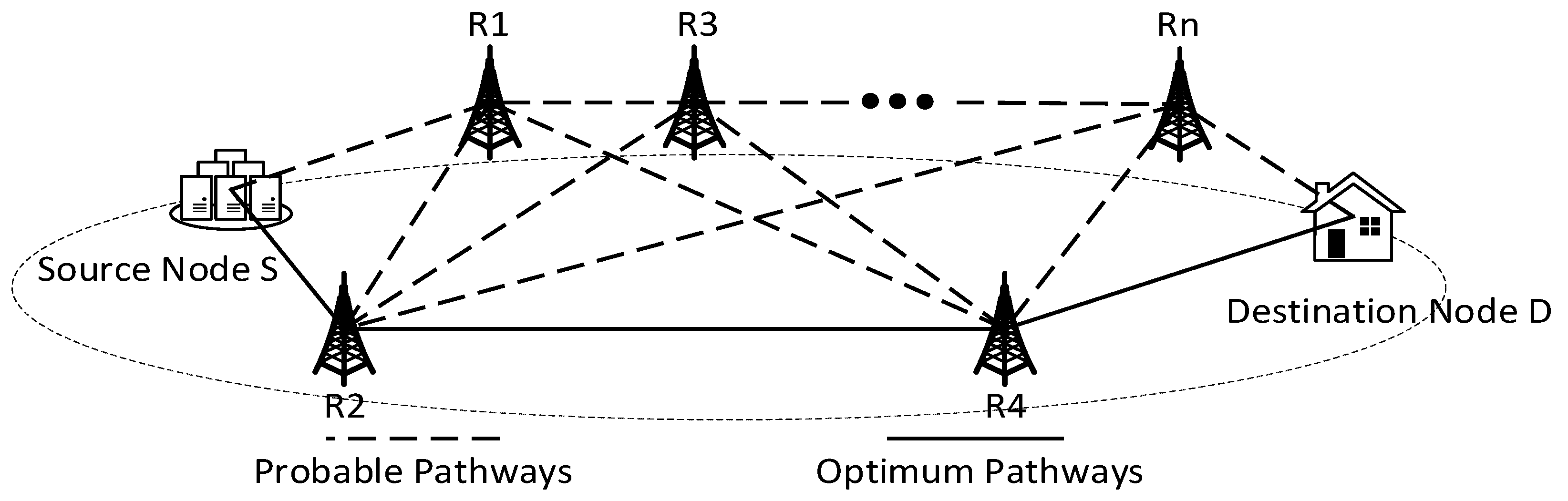
2.1. Description of the System Model

The wireless communication system model is a multi-hop relay network model based on a joint optimization strategy in a single source–single target scenario, as shown in Figure 1. The system model consists of three parts: source node $S$, which is responsible for sending the initial information; destination node $D$, which is responsible for receiving information; and $n$ relay nodes $R$ between source node S and destination node $D$, which undertake the task of enhancing and forwarding the signal, thus overcoming various obstacles in the transmission process. In this model, there are multiple alternative paths from source node $S$ to destination node $D$. How to determine a path that can not only optimize communication performance but also ensure the optimal distribution of energy efficiency has become the core research content of this paper.

2.2. System Performance Analysis

The system model possesses connectivity, which constitutes the basis for ensuring reliable information transmission within the power wireless private network. In the power system, the transmission of real-time monitoring data and control instructions must not be interrupted; otherwise, it might affect the stable operation of the power system and even trigger safety incidents. Let the node set in the network be $\nu =\left\{S,R_1,R_2,\cdot \cdot \cdot ,R_n,D\right\}$, in which $S$ is the source node, $D$ is the destination node, and $R_i$ is the i-th relay node. The set of communication links is $\epsilon$, constituting graph $G(\nu ,\epsilon )$. Since there is no direct connection link between $S$ and $D$, the connectivity of the system needs to satisfy the existence of at least one M-hop path $p=(S,R_{k_1},R_{k_2},\cdot \cdot \cdot ,R_{k_M},D)$ from $S$ to $D$, where $M\ge 1$ and $R_{k_i}\in \nu$; that is, the path has to contain at least one relay node. Introduce the adjacency matrix $A\in {ℝ}^{(n+2)\times (n+2)}$, where element $a_{ij}$ represents whether a direct connection link exists between node $i$ and node $j$. If it exists, it is $a_{ij}=1$; otherwise, it is 0. Based on assumption $a_{SD}=a_{DS}=0$, there is no direct connection link between $S$ and $D$. Whether a path of length $k$ exists can be determined through the power operation of the matrix, and the system connectivity needs to satisfy ${\displaystyle \sum _{k=2}^{n+1}{a}_{SD}^{(k)}}\ge 1$; that is, at least one valid path exists to ensure the continuity and reliability of the power operation.

The system model is capable of enhancing signal transmission. In the power wireless private network, due to the obstruction of power facilities and attenuation during the signal propagation process, the signal strength may be substantially weakened. The mechanism where the relay node is responsible for enhancing and forwarding signals can effectively overcome these transmission obstacles and ensure that the destination node receives a sufficiently strong signal. Let the signal power sent by source node $S$ be $P_S$ and the signal power received by the i-th relay node $R_i$ be

$$P_{R_i}^{\mathrm{recv}}=P_S\cdot {\gamma }_{S\to R_i}$$

(1)

The path-loss coefficient ${\gamma }_{S\to R_i}$ from $S$ to $R_i$ is associated with path-loss $L$ (refer to the model in Section 2.3). The specific calculation approach is as follows:

$${\gamma }_{S\to R_i}={10}^{-{\displaystyle \frac{L}{10}}}$$

(2)

The relay node amplifies the signal with an amplification factor of ${\alpha }_i$, and accordingly, its forwarding power is

$$P_{R_i}^{\mathrm{trans}}={\alpha }_i\cdot P_{R_i}^{\mathrm{recv}}$$

(3)

The power received by destination node $D$ from relay node $R_i$ amounts to

$$P_D^{\mathrm{recv}}=P_{R_i}^{\mathrm{trans}}\cdot {\gamma }_{R_i\to D}={\alpha }_i{P}_S{\gamma }_{S\to R_i}{\gamma }_{R_i\to D}$$

(4)

For the multi-hop path $p=(S,R_{k_1},R_{k_2},\cdot \cdot \cdot ,R_{k_M},D)$, the received power of $D$ as the cumulative outcome of each hop is

$$P_D^{\mathrm{recv}}=P_S{\displaystyle \mathbf{\prod }_{m=1}^M{\alpha }_{k_m}}{\gamma }_{k_{m-1}\to k_m}\cdot {\gamma }_{k_M\to D}$$

(5)

where $k_0=S$, $k_{M+1}=D$, and $M\ge 1$.

The system model possesses adaptability. The state of the power network undergoes dynamic changes along with load variations, equipment switching, and environmental interferences. The adaptability of the system model enables the network to adjust communication paths and signal processing approaches dynamically in accordance with these real-time variations. The link performance index ${\eta }_{ij}(t)$ and link load ${\rho }_{ij}(t)$ at moment $t$ are defined to, respectively, characterize the communication quality (such as the signal-to-noise ratio) and the resource occupancy rate from node $i$ to node $j$. The comprehensive performance index of path $p$ is

$$\Psi (p,t)={\omega }_{\eta }\cdot {\displaystyle \sum _{(i,j)\in p}{\eta }_{ij}}(t)-{\omega }_{\rho }\cdot {\displaystyle \sum _{(i,j)\in p}{\rho }_{ij}}(t)$$

(6)

where ${\omega }_{\eta },{\omega }_{\rho }\in [0,1]$ is a weighting coefficient, satisfying ${\omega }_{\eta }+{\omega }_{\rho }=1$. The system monitors $\Psi (p,t)$ in real time. If it drops below the threshold ${\Psi }_{th}$, it triggers path replanning and selects the optimal path $p^{*}$.

2.3. Objective Function

Based on the above system performance analysis, the key factors influencing communication quality and efficiency in the system model are defined, including the signal power, link communication performance, link load, etc. In the system model, the signal-to-interference-plus-noise ratio (SINR) of the transmitting and relaying nodes serves as a crucial indicator for measuring communication quality. It is closely related to the aforementioned factors and will directly impact the system’s overall performance and the subsequent optimization of the objective function. The channel SINR of the sending node and relay node can be expressed as

$$SIN{R}_i=\left\{\begin{array}{l}{\displaystyle \frac{P_s}{P_{N+I}}} \mathrm{Transmitting} \mathrm{Node}\\ {\displaystyle \frac{P_i}{P_{N+I}}} \mathrm{Relay} \mathrm{Node}\end{array}\right.$$

(7)

where $P_S$ represents the signal power sent by source node $S$, $P_i$ represents the signal power forwarded by the i-th relay node, and $P_{N+I}$ represents the power of noise and interference.

In the power wireless private network, the Okumura–Hata model [20] is chosen as the inter-node channel fading model, and its mathematical expression is

$$\begin{array}{l}L=69.55+26.16{\log }_{10}{f}_c-13.82{\log }_{10}{h}_b\\ +(44.9-6.55{\log }_{10}{h}_b){\log }_{10}d-\alpha (h_m)\end{array}$$

(8)

where $L$ represents path loss, with the unit being decibels, $f_c$ denotes the selected working frequency, which is 230 MHz in the power wireless private network, $h_b$ represents the height of the transmitting antenna, $h_r$ represents the height of the receiving antenna, d represents the distance between the sending and receiving sides, and $\alpha (h_r)$ is the correction factor of the antenna:

$$\alpha (h_r)=8.29{({\log }_{10}1.54h_r)}^2-1.1$$

(9)

The expression of the antenna correction factor $\alpha (h_r)$ in Formula (5) originates from the correction term of the Okumura–Hata model in the context of medium-sized and small cities. Reference [20] meticulously verified the applicability of this correction factor in the power context.

In multi-hop relay systems, energy efficiency is defined as the ratio of end-to-end throughput to total energy consumption, which can be expressed as [21]

$$EE={\displaystyle \frac{B\hspace{0.17em}{\log }_2\left[1+\underset{i}{\min }(SIN{R}_i)\right]}{P_O+P_S+{\displaystyle \sum _{i=1}^m{P}_i}}}$$

(10)

where $m$ represents the number of relay nodes in the communication link, and $P_O$ represents the power consumed in the system except for communication. The term $\underset{i}{\min }(SIN{R}_i)$ represents selection of the hop with the smallest SINR from the $m+1$ hops between source node $S$ and relay node $D$, thereby obtaining the minimum channel capacity among the $m+1$ hops. This minimum channel capacity is used to limit the information transmission rate; if the transmission rate exceeds this value, it may cause an interruption.

The mathematical issue of the joint optimization strategy, under constraints such as meeting the minimum transmission rate required for user service quality, node power limitations, and signal-to-interference ratio thresholds while maximizing the system energy efficiency, can be represented as

$$\begin{array}{l}\max {\displaystyle \frac{B\hspace{0.17em}{\log }_2\left[1+\underset{i}{\min }(SIN{R}_i)\right]}{P_O+P_S+{\displaystyle \sum _{i=1}^m{P}_i}}}\\ s.t. {\mathrm{C}}_1: P=\{P_S,P_i|i\in [1,m]\}\\ {\mathrm{C}}_2: 0<P\le P_C\\ {\mathrm{C}}_3: P_S+{\displaystyle \sum _{i=1}^m{P}_i}\le P_C\\ {\mathrm{C}}_4: B\hspace{0.17em}{\log }_2\left[1+\underset{i}{\min }(SIN{R}_i)\right]\ge r_0\\ {\mathrm{C}}_5: P-P_{N+I}-L\ge SIN{R}_{TH}\end{array}$$

(11)

where $P$ represents the set of transmitted power of each node, $P_C$ represents the maxi mum power that the node can provide, $r_0$ represents the minimum transmission rate that needs to be met in the power wireless private network, and $SIN{R}_{TH}$ represents the signal-to-interference-plus-noise ratio threshold.

The constraint conditions $C_2$ and $C_3$ stipulate the upper and lower bounds of the transmission power of each node and the upper bound of the total transmission power of all nodes. The constraint condition $C_4$ ensures that the transmission rate of the system satisfies the requirements of the user’s quality of service. The constraint condition $C_5$ guarantees that the link will not be interrupted. The left side of the inequality represents the received signal-to-interference ratio of each hop, which is obtained by calculating the transmission loss of each hop.

Theorem 1. 

For the definite parameter $B, P_{N+I}, P_O, P_C, r_0, L, SIN{R}_{TH}$, the maximum value of the objective function must exist.

Proof of Theorem 1. 

See Appendix A for details. □

When solving the above optimization problem with traditional methods, the difficulty increases with the addition of relay nodes. Therefore, the energy efficiency optimization problem is decomposed into two subproblems: relay selection and power control.

3. Algorithm Design and Implementation

The proposed FD-Dink energy efficiency optimization algorithm achieves the joint optimization of relay selection and power control via a hierarchical framework. To begin with, based on the dense distribution characteristics of the nodes in the power private network, the geometric coverage model is adopted to pre-screen the candidate nodes and retain the core candidate node set to reduce the computational complexity of the subsequent algorithms. On this basis, the modified D* algorithm substitutes the traditional distance heuristic function with path loss and dynamically selects the multi-hop path with the minimum transmission loss in combination with the Okumura–Hata channel model of the power grid scenario. When there are no available nodes in the pre-screening area, the algorithm switches to the hop-by-hop forward maximum signal-to-noise ratio (FMSNR) mode, guaranteeing link reliability through hop-by-hop optimal relay selection. After the pre-screening narrows the solution space, the improved D* algorithm generates low-loss paths, while the FMSNR mechanism offers redundancy and fault tolerance, jointly achieving adaptive path planning in dynamic environments. Finally, the non-convex energy efficiency optimization problem is transformed into a linear subproblem by the Dinkelbach method. The energy efficiency weight parameter is updated in the outer iteration, and the Lagrange multiplier method is utilized in the inner iteration to dynamically adjust the multipliers, rapidly converging to a power allocation scheme that satisfies the QoS constraints. By combining the path-loss parameters and the planning results of the modified D* algorithm, the algorithm achieves the joint optimization of the power and paths through an outer–inner double-layer iteration.

Node pre-screening generates a streamlined candidate set. The improved D* and FMSNR ensure path reliability and low levels of loss. The power control module optimizes the energy efficiency configuration based on dynamic parameters. Through the coupling relationship between path loss and transmission power, these three significantly reduce the computational complexity and transmission delay, ultimately maximizing the global energy efficiency of the system.

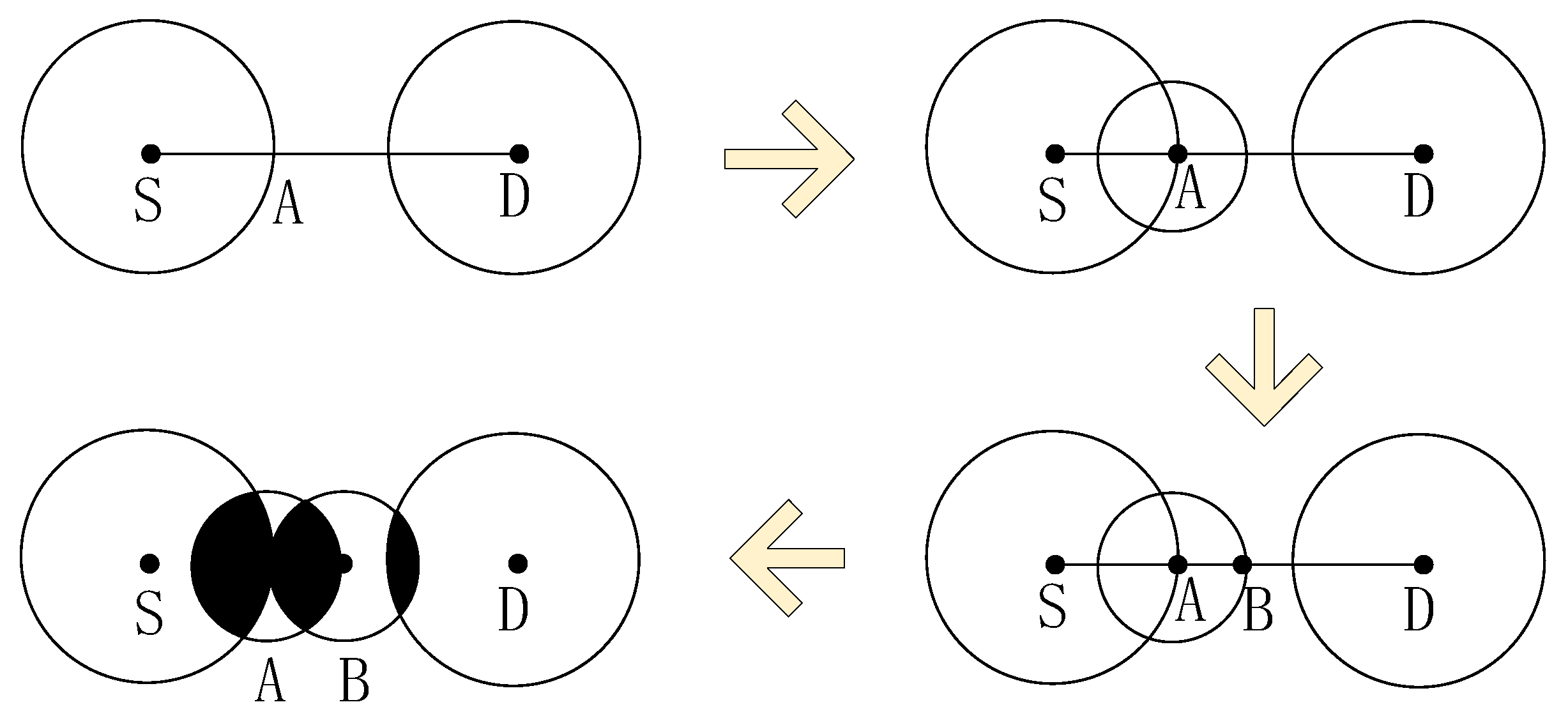
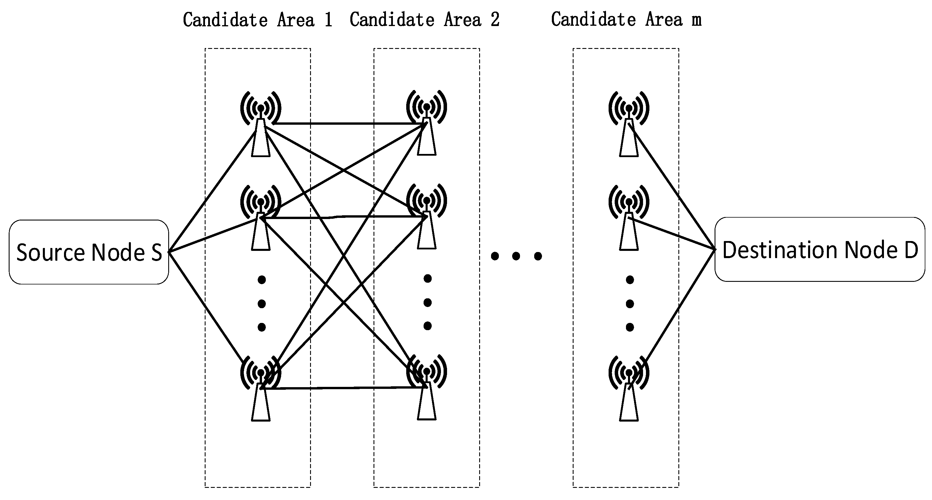
3.1. Node Pre-Screening

Node pre-screening, the first step of the FD-Dink algorithm, determines candidate regions based on node coverage (related to signal power and transmission loss) with a maximum radius $d_{\max }$. If the received SINR falls below a certain threshold, which is set at 0 dB in this paper, the link is regarded as interrupted. According to the formula

$$P-P_{N+I}-L=0$$

(12)

the maximum coverage of node $d_{\max }$ can be obtained.

With source node $S$ and target node $D$ as the geometric center and $d_{\max }$ as the radius, a circular region is constructed to define the $d_{\max }$ physical coverage of the node. Since there is no direct link between $S$ and $D$, only the case of two circles being separated is considered here, as shown in Figure 2.

In the case where the two circles are mutually disjointed, the intersection point A of the line segment SD and $O_S$ is determined first. Subsequently, based on point A, a circular region with a diameter of $d_{\max }$ is constructed and denoted as $O_A$. Next, whether $O_A$ intersects with the original two circles is determined. Conversely, if $O_A$ has no intersection with the original two circles, the intersection points of line segment AD and the two circles are marked as B. Based on point B, a circular area with a diameter of $d_{\max }$ is constructed and denoted as $O_B$. The process iterates until overlapping regions contain candidate nodes. Once the condition is satisfied, the screening process comes to an end. Eventually, all the nodes located within the shaded area depicted in Figure 2, that is, within the intersection of the two circles, are affirmed as potential nodes.

After the node pre-screening operation is completed, the system model can be transformed into the form shown in Figure 3.

3.2. The Improved D* Algorithm in Combination with FMSNR

The D* algorithm, a dynamic path-planning method, aligns with the system’s adaptability by enabling real-time path adjustments. The cost formula of the D* algorithm extends the A* algorithm [22]

$$f(n)=h(n)+km(n)$$

(13)

where h(n) represents the generation value from the current point to the target, and km(n) is used to record the minimum generation value in the current node. The algorithm prioritizes nodes based on updated cost values.

To address the inaccuracy of distance-based heuristics in power scenarios, the D* algorithm substitutes the distance factor with path loss. The cost formula can be expressed as

$$\begin{array}{l}f(n)=(69.55+26.16{\log }_{10}{f}_c-13.82{\log }_{10}{h}_b+\\ (44.9-6.55{\log }_{10}{h}_b){\log }_{10}d-\alpha (h_m))+\alpha \times km(n)\end{array}$$

(14)

Path loss is calculated via the Okumura–Hata model. Only when path loss is sufficiently small can the transmission power of each node be maintained at a relatively low level and not be interrupted due to being less than the threshold signal-to-interference ratio. The comprehensive implementation steps of the D* algorithm based on path loss, are formally delineated in Algorithm 1.

Algorithm 1. The D* algorithm based on path loss

Initialize two lists: open_set and close_set, where open_set is used to store the nodes to be explored and close_set is used to store the nodes that have already been processed. Initialize open_set and close_set. Add the starting point to open_set with a priority of 0. If open_set is not empty, select the node n with the highest priority. If n is the end point, trace the parent node to generate a path, and the algorithm ends; otherwise, execute the content of 5 in the number list. Move n from open_set to close_set and traverse the adjacent node m. For each neighboring node m, skip if m is already in close_set; otherwise, calculate the cost of the new path from the current node n to m (including the path loss). If m is not in open_set, set the parent node of m to n, calculate its priority, and add it to open_set; if m is already in open_set and the newly calculated path cost is lower than its original priority, update m’s parent node to n, recalculate its priority, and adjust its order in open_set. Return to number 3 in the list of numbers until a path is found or the open_set is empty.

In scenarios with insufficient node density, the pre-screening process may yield no viable relay nodes, leading to communication interruptions. In order to avoid such problems, an integrated strategy is adopted that combines the optimized D* algorithm based on node pre-screening with the forward maximum signal–noise ratio (FMSNR) algorithm.

The principle of the FMSNR algorithm is to select the relay node that can provide the maximum forward signal–noise ratio in each hop so as to ensure the transmission quality of the signal in each hop. The integration of these algorithms leverages the dynamic path-planning capabilities of D* for rapid route optimization while ensuring signal quality through FMSNR-based criteria so as to improve the performance and reliability of the whole communication system. The detailed implementation steps of the improved D* algorithm in combination with FMSNR, are formally delineated in Algorithm 2.

Algorithm 2. The improved D* algorithm in combination with FMSNR

Based on the location information of relay nodes, the selected nodes are pre-screened and divided into multiple candidate regions. Check whether each candidate area contains selectable nodes. If all areas include selectable nodes, execute the content numbered 3 in the list; otherwise, execute the content numbered 4 in the list. The improved D* algorithm is used to perform global optimization decisions on the selected relay nodes, determine the optimal relay node in the distributed candidate region, and achieve the optimal configuration of communication links to complete collaborative communication, and the algorithm is terminated. For a relay node set that did not pass the pre-screening, the FMSNR algorithm is executed to determine the relay node, achieve the optimal configuration of the communication link, and complete the cooperative communication, and the algorithm is terminated.

3.3. The Power Control Algorithm Based on the Dinkelbach Method and the Lagrange Multiplier Method

After determining the relay selection, power control is the key to maximize the energy efficiency of the system. According to reference [21], the maximum energy efficiency can be obtained when the power of the nodes is equal. The original objective function can be converted to

$$\begin{array}{l}\max {\displaystyle \frac{B\hspace{0.17em}{\log }_2\left[1+\frac{P_S}{P_{N+I}}\right]}{P_O+(m+1)P_S}}\\ s.t.{\mathrm{C}}_1: 0<P_S\le P_C\\ {\mathrm{C}}_2: 0<(m+1)P_S\le P_C\\ {\mathrm{C}}_3: B\hspace{0.17em}{\log }_2\left[1+{\displaystyle \frac{P_S}{P_{N+I}}}\right]\ge r_0\end{array}$$

(15)

The concave function in the fractional form presented in Formula (15) is transformed by means of the Dinkelbach method. The basic idea of the Dinkelbach method is to transform the original problem into a series of convex optimization subproblems by introducing an auxiliary variable. In each iteration, the optimal solution of the original problem is gradually approximated according to the updated value of the solution of the subproblem.

Theorem 2. 

For the given parameter $B$, $P_{N+I}$, $P_O$, the objective function is a strictly concave function concerning the variables $P_S$ and $\forall m$.

Proof of Theorem 2. 

See Appendix B for details. □

The maximum energy efficiency as indicated in Formula (15) is

$$w^{*}={\displaystyle \frac{B\hspace{0.17em}{\log }_2\left[1+\frac{P_S^{*}}{P_{N+I}}\right]}{P_O+(m+1)P_S^{*}}}$$

(16)

where the variable $w^{*}$ represents the energy efficiency value from the transmitting end to the receiving end, and $P_S^{*}$ is the transmitting power of the source node when the energy efficiency reaches the maximum value. It is known from the literature [23] that Lemma 1 is valid.

Lemma 1. 

$w^{*}$ is obtained if, and only if, the following conditions are true:

$$\begin{array}{l}\underset{P_S}{\max }\left\{B\hspace{0.17em}{\log }_2\left[1+{\displaystyle \frac{P_S}{P_{N+I}}}\right]-w^{*}\left[P_O+(m+1)P_S\right]\right\}=\\ B\hspace{0.17em}{\log }_2\left[1+{\displaystyle \frac{P_S^{*}}{P_{N+I}}}\right]-w^{*}\left[P_O+(m+1)P_S^{*}\right]=0\end{array}$$

(17)

Proof of Lemma 1. 

For the proof procedure refer to reference [23]. □

According to Lemma 1, the optimization problem can be transformed into the following form:

$$\begin{array}{l}\underset{P_S}{\max }\left\{B\hspace{0.17em}{\log }_2\left[1+{\displaystyle \frac{P_S}{P_{N+I}}}\right]-w^{*}\left[P_O+(m+1)P_S\right]\right\}\\ s.t.{\mathrm{C}}_1: 0<P_S\le P_C\\ {\mathrm{C}}_2: 0<(m+1)P_S\le P_C\\ {\mathrm{C}}_3: B\hspace{0.17em}{\log }_2\left[1+{\displaystyle \frac{P_S}{P_{N+I}}}\right]\ge r_0\end{array}$$

(18)

Here, the iterative approach is employed to obtain the value of $w^{*}$. During the nth iteration process, when power takes the value of $P_S(n)$ and energy efficiency takes the value of $w(n-1)$, the augmented Lagrangian corresponding to Formula (18) can be represented as

$$\begin{array}{l}L(P_S,\delta ,\theta ,\mu )=B\hspace{0.17em}{\log }_2\left[1+{\displaystyle \frac{P_S(n)}{P_{N+I}}}\right]-w(n-1)\left[P_O+(m+1)P_S(n)\right]-\\ \delta (n)\left[P_S(n)-P_C\right]-\theta (n)\left[(m+1)P_S(n)-P_C\right]+\mu (n)\left[B {\log }_2\left(1+{\displaystyle \frac{P_S}{P_{N+I}}}\right)-r_0\right]\end{array}$$

(19)

where $\delta (n)$, $\theta (n)$, and $\mu (n)$ are Lagrangian operators of constraint expressions that are used to deal with constraints. When the node power approaches its maximum allowable power, the corresponding Lagrange multipliers $\delta (n)$ and $\theta (n)$ will increase, thereby adding a penalty term in the objective function and impelling the algorithm to search for the optimal solution that meets the power constraints. When the link transmission rate is lower than the minimum requirement $r_0$, $\mu (n)$ will increase, causing the objective function to optimize to enhance the transmission rate. In this way, the Lagrange multiplier method can ensure that under the premise of meeting all constraints, the optimal power allocation can be achieved to achieve the goal of maximizing the energy efficiency of the system.

According to the Lagrange dual decomposition, the energy efficiency optimization problem of the equation is equivalent to

$$\underset{(\delta ,\theta ,\mu \ge 0)}{\min }\underset{P_S}{\max } L(P_S,\delta ,\theta ,\mu )$$

(20)

which can be obtained by the KKT condition:

$$\stackrel{\wedge }{P_S}(n)={\left\{{\displaystyle \frac{\left[1+\mu (n)\right]B\hspace{0.17em}{\log }_{2}e}{(m+1)[w(n-1)+\theta (n)]+\delta (n)}}-P_{N+I}\right\}}^{+}$$

(21)

In the formula ${\{\cdot \}}^{+}=\max \{0,\cdot \}$, the values of the Lagrange multipliers $\delta (n)$, $\theta (n)$, and $\mu (n)$ can be updated iteratively through the gradient descent method:

$$\delta (n,\tau +1)={\left\{\delta (n,\tau )+\alpha \left[\stackrel{\wedge }{P_S}(n,\tau )-P_C\right]\right\}}^{+}$$

(22)

$$\theta (n,\tau +1)={\left\{\theta (n,\tau )+\alpha \left[(m+1)\stackrel{\wedge }{P_S}(n,\tau )-P_C\right]\right\}}^{+}$$

(23)

$$\begin{array}{l}\mu (n,\tau +1)={\left\{\mu (n,\tau )-\alpha \left[B\hspace{0.17em}{\log }_2\left(1+{\displaystyle \frac{\stackrel{\wedge }{P_S}(n)}{P_{N+I}}}\right)-r_0\right]\right\}}^{+}\\ \end{array}$$

(24)

where $\tau$ denotes the $\tau$-th iteration of the Lagrange operator, and $\alpha$ is the step size.

When solving the power allocation problem, a two-layer iteration mechanism is constructed, and the optimal solution is gradually approximated by alternating iterations of the inner and outer layers. During the outer iteration process, the goal is to solve parameter w. The number of iterations in each round is denoted as n, the maximum number of iterations is set to $I_{outer}$, and the convergence threshold is ${\Delta }_1$. The inner iteration focuses on updating the Lagrange multipliers $\delta$, $\theta$, and $\mu$. The number of iterations in each round is represented by $\tau$, the maximum number of iterations is set to $I_{inner}$, and the convergence threshold is ${\Delta }_2$. The complete procedures of this algorithm are presented as Algorithm 3.

Algorithm 3. The power allocation algorithm based on the Dinkelbach method and the Lagrange multiplier method

The pseudocode is detailed in Appendix C. Set the iteration counter n to 1 and $\tau$ to 0. Initialize the variables required for the algorithm, encompassing $w(n)$$, \delta (n,\tau )$$, \theta (n,\tau )$$, \mu (n,\tau )$, and the iteration counts $I_{outer}$ and $I_{inner}$. Initialize the convergence thresholds ${\Delta }_1$ and ${\Delta }_2$. When n is smaller than $I_{outer}$, the number of iterations of the outer loop is executed. Calculate $\stackrel{\wedge }{P_S}(n)$ based on the formula. If the discrepancy between the calculated power $\stackrel{\wedge }{P_S}(n)$ and the power from the previous iteration is less than ${\Delta }_1$, update the optimal power $P_S^{*}$ to the current $\stackrel{\wedge }{P_S}(n)$ and break out of the loop. If the power update condition is not fulfilled, the inner loop is accessed. Execution occurs when $\tau$ is less than the inner iteration count $I_{inner}$. Within the inner loop, the Lagrangian multiplier and the power of the current iteration are configured to be identical to those of the previous iteration. If the discrepancy between the Lagrange multipliers and power of the current iteration and those of the previous iteration is less than ${\Delta }_2$, update the Lagrange multipliers $\delta (n,\tau )$, $\theta (n,\tau )$, and $\mu (n,\tau )$ and power $\stackrel{\wedge }{P_S}(n,\tau )$. Calculate the weights $w(n-1)$. If the inner loop is accomplished, increment the value of $\tau$ and proceed to the next inner loop. If the inner loop fulfills the condition, break out of the inner loop. If the inner loop is complete, increase the value of n to continue the next outer loop. When the outer loop is completed, the algorithm ends and outputs the optimal weight $w^{*}$ and the optimal power $P_S^{*}$.

To sum up, in the algorithm design, the improved D* algorithm in conjunction with FMSNR is capable of enhancing the communication reliability and energy efficiency of the path through superior relay selection. The power control algorithm based on the Dinkelbach approach and the Lagrange multiplier method, through precise power allocation, minimizes the total power consumption of the system while meeting the system’s quality of service requirements, further enhancing the system’s energy efficiency and jointly achieving the collaborative optimization of communication performance and energy efficiency in the power wireless private network.

4. Case Implementation and Analysis

4.1. Case Parameter Setting

Employing the MATLAB R2024a platform, the performance of the energy efficiency optimization algorithm was assessed via 1000 Monte Carlo experiments. During each experimental run, the relay nodes within the system model were deployed in a random distribution manner. The primary simulation parameters are presented in

Table 1. Parameter settings.

Parameters	Numerical Values
Communication bandwidth $B$/MHz	1
Node power range $P$/dBm	[10, 40]
Rest communication power $P_O$/dBm	10
Noise power $P_{N+I}$/dBm	−114
Minimum transfer rate $r_0$/($\mathrm{bit}\cdot {\mathrm{s}}^{-1}$)	5
Cell range/${\mathrm{m}}^2$	4000 × 4000
Distance between nodes/km	4
Base station antenna height $h_b$/m	35
Terminal antenna height $h_r$/m	1.2
Number of network relay nodes/pieces	10–100

.

4.2. Algorithm Flow

The flowchart of the FD-Dink energy efficiency optimization algorithm is shown in Figure 4. When the FD-Dink energy efficiency optimization algorithm is executed, the relay selection is initially configured. Then, node coverage is determined based on signal power, transmission loss, and other factors, followed by node pre-screening. Subsequently, it checks whether there are any selectable nodes in each area after pre-screening. If so, the improved D* algorithm combined with FMSNR is employed. By comprehensively considering path loss and signal quality, the optimal relay node is determined. If not, the FMSNR algorithm is used to complete the relay selection. After the relay selection, the power control phase is entered. First, power control is initialized, and the initial power value is set. After the outer iteration, the calculated power is compared with the previous power each time to determine whether the convergence conditions are met. If not, the inner iteration is entered, the Lagrange multiplier is updated, and the power is updated when the inner layer reaches the convergence condition. The inner and outer layers are alternately iterated until the outer iterations satisfy the convergence requirements. The final output is the optimal power and energy efficiency that can maximize the system’s energy efficiency.

4.3. Case Study

In the process of relay selection, the nodes need to be pre-screened, as shown in Figure 5. In the square cell area with a side length of 4000 m, 100 nodes are randomly and evenly distributed. In the pre-screening stage, a large number of nodes are screened. After screening, only efficient nodes located in the core area are retained to form a new node set from the node group that was originally densely distributed in the region. Statistical analysis indicates that approximately 70% of redundant nodes are eliminated during pre-screening, thereby substantially enhancing network efficiency. Through this screening operation, the communication efficiency of the network is significantly improved, the energy utilization efficiency is also enhanced, and the degree of redundancy in the network is greatly reduced so that the performance of the entire network is optimized.

Figure 6 illustrates the variation in outage probability as it changes with the number of relay nodes in the network. Through a comparative analysis of the interruption probability between the A* relay selection algorithm mentioned in reference [13] and the algorithm proposed in this paper, it can be observed that the interruption probabilities of the FMSNR algorithm, the FMSNR-A* algorithm, and the FMSNR-D* algorithm are consistently lower than that of the D* algorithm. The interruption probabilities of the FMSNR algorithm, FMSNR-A* algorithm, and FMSNR-D* algorithm are consistently lower than that of the D* algorithm. The higher outage probability of the D* algorithm stems from low node density, which may result in no nodes in the region remaining after node pre-screening. When the number of nodes in the network ranges from 10 to 30, the FMSNR-A* and FMSNR-D* algorithms primarily switch to the FMSNR-based mode. When the number of relay nodes in the network exceeds 40, the four different algorithms exhibit consistent interruption probabilities, indicating that in high-density node environments, the differences between the algorithms are offset by the network’s redundancy. Therefore, in high-density scenarios, the algorithm complexity can be appropriately simplified to reduce energy consumption. In summary, when the distance between users reaches 4000 m, the FMSNR-D* algorithm demonstrates the best performance in link interruption probability control through its adaptive path-optimization mechanism.

Figure 7 depicts the trend of the number of relay hops changing along with the quantity of network relay nodes. Through a contrastive analysis of the delay with the A* relay selection algorithm referred to in reference [13], it can be observed that as the number of network relay nodes increases, the number of relay nodes selected by the FMSNR algorithm positively correlates with the network scale. However, during this process, the number of hops of the D* algorithm remains stable, mainly because its hop selection is primarily influenced by the end-to-end physical distance. Further study of the transmission delay characteristics shows that when the number of nodes in the network is in the range of 10–30, there may be no nodes in the selected area due to the network layout and other factors. In this case, FMSNR-D* and FMSNR-A* algorithms will automatically switch to the working mode dominated by the FMSNR algorithm. According to the experimental results, the path-planning efficiency of the FMSNR-D* algorithm is significantly higher than that of the FMSNR-A* algorithm, which means that it can find the appropriate relay node more quickly and efficiently and optimize the communication path. When the number of network relay nodes exceeds 30, the performance of the D*, FMSNR-A*, and FMSNR-D* algorithms gradually becomes the same. This phenomenon shows that in the case of a large number of network nodes, the differences between different algorithms are masked by the complexity and redundancy of the network. In summary, the FMSNR-D* algorithm has excellent performance in delay control under the specific condition that the user distance reaches 4000 m. It can significantly improve the timing stability during long-distance transmission, ensuring that data can be more stable and the transmission efficient.

When the number of nodes lies within the range of 10 to 30, diverse relay selection algorithms demonstrate disparate performance manifestations, as presented in

Table 2. Performance analysis of different relay selection algorithms.

Schemes	Interrupt Probability	Number of Relay Hops
D*	0.136	3
FMSNR-A*	0.051	5
FMSNR-D*	0.048	4
FMSNR	0.031	9

. This table primarily conducts an analysis of multiple relay selection algorithms in terms of two crucial performance indicators, namely, interruption probability and relay hop number. On the whole, when the number of nodes is within the range of 10 to 30, the FMSNR-D* algorithm exhibits the best performance.

Figure 8 illustrates how energy efficiency varies with transmit power under different relay hops. As indicated by the data trend, there is a significant negative correlation between system energy efficiency and transmit power. According to Shannon’s theorem, channel capacity increases logarithmically with power, while energy consumption increases linearly with power. The growth rate of energy consumption far exceeds that of channel capacity, directly resulting in a continuous decrease in unit energy transmission efficiency. Additionally, when there are more relay hops in the network, the signal must pass through more relay nodes during transmission. Each time the signal goes through a relay node, additional energy is consumed, and signal attenuation during transmission is correspondingly increased. These factors compound each other, leading to an even more pronounced decline in the system’s energy efficiency.

Figure 9 presents the correlation characteristics between system energy efficiency and the number of relay hops under various common power allocation strategies and conducts a comparative analysis with the iterative water-filling algorithm proposed in reference [15]. In multi-hop relay networks, the decline in system energy efficiency is primarily attributed to two crucial factors. Firstly, as the number of relay hops increases, the path loss and multipath interference endured by the signal during transmission intensify exponentially. To maintain the signal transmission quality, more energy is required to compensate for channel attenuation, thereby reducing energy efficiency. Secondly, each relay node consumes energy during operations such as baseband processing and radio frequency conversion. With the increase in the number of hops, the energy consumption of these circuits accumulates continuously, further lowering the system’s energy efficiency. Regarding the power allocation strategies, the equal power allocation scheme disregards the channel differences among individual nodes and allocates the same power to all nodes. This leads to excessive energy consumption at nodes in deep fading channels to guarantee signal transmission, while at nodes with superior channels, the allocated power exceeds the actual demand, resulting in power redundancy. Consequently, the overall energy efficiency curve of the system under the equal power allocation scheme remains at a low level from the outset, failing to achieve efficient energy utilization and having the lowest energy efficiency. Although the power allocation scheme based on channel gain optimizes the power of each single-hop link, it lacks a global perspective in multi-hop transmission scenarios and does not consider the constraint effect of backward hops on forward power allocation, resulting in limited energy efficiency gains. In dynamic multi-hop scenarios, the iterative convergence direction of the iterative water-filling algorithm deviates from the global energy efficiency surface and is prone to being trapped in local suboptimal solutions, with its overall performance being inferior to the algorithm proposed in this paper.

Table 3. Performance analysis of different power allocation schemes.

Number of Relay Hops	The Scheme in This Paper Is Relative to the Power Allocation Efficiency Increase Rate Based on Channel Gain	The Scheme in This Paper Is Relative to the Equal Power Allocation Efficiency Increase Rate	The Scheme in This Paper Is Relative to the Iterative Water-Filling Algorithm Efficiency Increase Rate
1	9%	29%	5%
2	13%	36%	7%
3	15%	46%	10%
4	20%	59%	12%
5	20%	60%	13%
6	20%	65%	14%
7	18%	66%	13%
8	21%	69%	15%
9	22%	73%	16%
10	26%	83%	18%

presents a more distinct comparison of the energy efficiency performances of different power allocation schemes. Through the collation and analysis of the energy efficiency data of each scheme under various relay hop counts, the energy efficiency improvement rates of the proposed scheme in this paper relative to the other three schemes are calculated, thereby visually demonstrating the advantages and characteristics of the proposed scheme in terms of energy efficiency. On the whole, the scheme proposed in this paper, by dynamically adjusting the power allocation, can better adapt to network variations and optimize the energy efficiency performance with more prominent advantages.

5. Conclusions

This study investigates energy efficiency optimization in multi-hop relay networks through a joint relay selection and power allocation strategy. The relay selection and power allocation problems are integrated for optimization, and the energy efficiency optimization problem is modeled under the condition of ensuring user QoS. The improved D* algorithm based on FMSNR is employed to address the dynamic relay selection problem. Once the relay selection is determined, the Dinkelbach method and Lagrange multiplier method are utilized to solve the optimal energy efficiency value by controlling the node transmission power. Comparative evaluations confirm the superiority of the proposed algorithm through existing methods in terms of outage probability, transmission delay, and energy efficiency, effectively resolving the issues of large node search space and significant transmission delay, thereby enhancing the overall energy efficiency of the system in multi-hop relay networks. Future research could integrate intelligent reflecting surface (IRS) technology and the federated learning framework to explore dynamic energy efficiency optimization under new energy power supply architectures. Furthermore, it is necessary to conduct in-depth research on digital twin-driven network energy efficiency prediction methods, providing novel insights for the sustainable development of power wireless private networks.

References

1. Zheng, C.; Wu, X.; Li, X.; Chen, J.; Lin, Z.; Xiao, Z.; Liu, H. Development of a 230 MHz Interference Source Identification Device for Power Wireless Private Networks. Procedia Comput. Sci. 2022, 203, 350–355. [Google Scholar]
2. Zhao, X.; Gan, J.; Xu, W.; Huang, T. A Covariance Matrix-Based Cooperative Spectrum Sensing Algorithm in Electric Wireless Private Network. Mob. Inf. Syst. 2022, 2022, 1420539. [Google Scholar] [CrossRef]
3. Li, A.; Liu, L.; Lv, Y.; Bai, Y.; Cui, L. Adaptability Analysis of Wireless Communication Application Scenarios Under New Power Systems. In Proceedings of the 2023 IEEE 11th Joint International Information Technology and Artificial Intelligence Conference (ITAIC), Chongqing, China, 8–10 December 2023; pp. 1588–1592. [Google Scholar]
4. Ma, L.; Li, W.; Hou, Y.; Yang, R.; Jia, W.; Qiu, Y. Application of wireless communication technology in ubiquitous power internet of things. In Proceedings of the 2020 IEEE 3rd International Conference on Computer and Communication Engineering Technology (CCET), Beijing, China, 14–16 August 2020; pp. 267–271. [Google Scholar]
5. Betriu, P.; Soria, M.; Gutiérrez, J.L.; Llopis, M.; Barlabé, A. An assessment of different relay network topologies to improve Earth–Mars communications. Acta Astronaut. 2023, 206, 72–88. [Google Scholar] [CrossRef]
6. Mahapatra, S.N.; Singh, B.K.; Kumar, V. A secure multi-hop relay node selection scheme based data transmission in wireless ad-hoc network via block chain. Multimed. Tools Appl. 2022, 81, 18343–18373. [Google Scholar] [CrossRef]
7. Sun, H.; Naraghi-Pour, M.; Sheng, W.; Han, Y. Performance Analysis of Incremental Relaying in Multi-Hop Relay Networks. IEEE Access 2020, 8, 68747–68761. [Google Scholar] [CrossRef]
8. Yuan, L.; Zhou, F.; Wu, Q.; Ng, D.W.K. Channel Prediction-Enhanced Intelligent Resource Allocation for Dynamic Spectrum-Sharing Networks. In Proceedings of the ICC 2024-IEEE International Conference on Communications, Denver, CO, USA, 9–13 June 2024; pp. 2767–2772. [Google Scholar]
9. Alvi, A.S.; Hussain, R.; Hasan, U.Q.; Malik, S.A. Improved Buffer-Aided Multi-Hop Relaying with Reduced Outage and Packet Delay in Cognitive Radio Networks. Electronics 2019, 8, 895. [Google Scholar] [CrossRef]
10. Zhao, Y.; Liu, X.; Liu, H.; Wang, X.; Huang, L. RIS-Aided MmWave Hybrid Relay Network Based on Multi-Agent Deep Reinforcement Learning. Mob. Netw. Appl. 2024, 29, 825–840. [Google Scholar] [CrossRef]
11. Dai, J.; Li, X.; Han, S.; Liu, Z.; Zhao, H.; Yan, L. Multi-hop relay selection for underwater acoustic sensor networks: A dynamic combinatorial multi-armed bandit learning approach. Comput. Netw. 2024, 242, 110242. [Google Scholar] [CrossRef]
12. Kravchuk, S.; Afanasieva, L. “Best” relay selection algorithm for wireless networks with cooperative relaying. In Proceedings of the 2019 International Conference on Information and Telecommunication Technologies and Radio Electronics (UkrMiCo), Odessa, Ukraine, 9–13 September 2019; pp. 1–4. [Google Scholar]
13. Li, Q.L.; Dou, Z.; Li, Z.G.; He, Q.H. Adaptive Relay Selection Algorithm for Maritime Multi-hop Communication Networks. In Proceedings of the 2022 National Microwave and Millimeter Wave Conference (Volume II), Harbin, China, 12 August 2022. (In Chinese). [Google Scholar] [CrossRef]
14. Zhang, G.; Yan, H.; Zeng, Y.; Cui, M.; Liu, Y. Trajectory optimization and power allocation for multi-hop UAV relaying communications. IEEE Access 2018, 6, 48566–48576. [Google Scholar] [CrossRef]
15. Khodmi, A.; Benrejeb, S.; Choukair, Z. Iterative water filling power allocation and relay selection based on two-hop relay in 5G/heterogeneous ultra dense network. In Proceedings of the 2018 Seventh International Conference on Communications and Networking (ComNet), Hammamet, Tunisia, 1–3 November 2018; pp. 1–6. [Google Scholar]
16. Zhu, J.; Xie, Z.; Jiang, Z.; Lin, P.; Zhu, J.; She, X.; Chen, P. A Joint Relay Selection and Power Allocation Strategy for Multi-Hop D2D Communications. In Proceedings of the 2024 IEEE/CIC International Conference on Communications in China (ICCC), Hangzhou, China, 7–9 August 2024; pp. 1087–1091. [Google Scholar]
17. Basak, S.; Acharya, T. Spectrum-aware outage minimizing cooperative routing in cognitive radio sensor networks. Wirel. Netw. 2020, 26, 1069–1084. [Google Scholar] [CrossRef]
18. Wang, X.; Jin, T.; Qian, Z.H.; Hu, L.S.; Wang, X. Research on Energy Efficiency Optimization Algorithm for D2D Relay-assisted Communication. J. Commun. 2020, 41, 71–79. (In Chinese) [Google Scholar]
19. Zhang, S.B.; Chen, C.; Li, Y. Power Control Algorithm for Multi-hop Relay Communication System Based on Energy Efficiency and Delay. J. Nanjing Univ. Posts Telecommun. Nat. Sci. Ed. 2021, 41, 1–8. (In Chinese) [Google Scholar] [CrossRef]
20. Akande, A.O.; Agubor, C.K.; Semire, F.A.; Akinde, O.K.; Adeyemo, Z.K. Intelligent Empirical Model for Interference Mitigation in 5G Mobile Network at Sub-6 GHz Transmission Frequency. Int. J. Wirel. Inf. Netw. 2023, 30, 287–305. [Google Scholar] [CrossRef]
21. Wang, R.; Liu, J.; Zhang, G.; Huang, S.; Yuan, M. Energy Efficient Power Allocation for Relay-Aided D2D Communications in 5G Networks. China Commun. 2017, 14, 54–64. [Google Scholar] [CrossRef]
22. Suanpang, P.; Jamjuntr, P. Optimizing Autonomous UAV Navigation with D* Algorithm for Sustainable Development. Sustainability 2024, 16, 7867. [Google Scholar] [CrossRef]
23. Dinkelbach, W. On nonlinear fractional programming. Manag. Sci. 1967, 13, 492–498. [Google Scholar] [CrossRef]
Figure 1. Multi-hop relay network model based on a joint optimization strategy.
Electronics 14 02017 g001
Figure 2. Pre-screening of the phase separation case.
Electronics 14 02017 g002
Figure 3. Trunk selection model.
Electronics 14 02017 g003
Figure 4. Flowchart of the FD-Dink energy efficiency optimization algorithm.
Electronics 14 02017 g004
Figure 5. Node distribution after node pre-screening.
Electronics 14 02017 g005
Figure 6. Outage probability vs. the number of relay nodes.
Electronics 14 02017 g006
Figure 7. The number of relay hops varies with the number of relay nodes in the network.
Electronics 14 02017 g007
Figure 8. Changes in energy efficiency with transmit power under different relay hops.
Electronics 14 02017 g008
Figure 9. Variation in energy efficiency with relay hops under different power allocation schemes.
Electronics 14 02017 g009