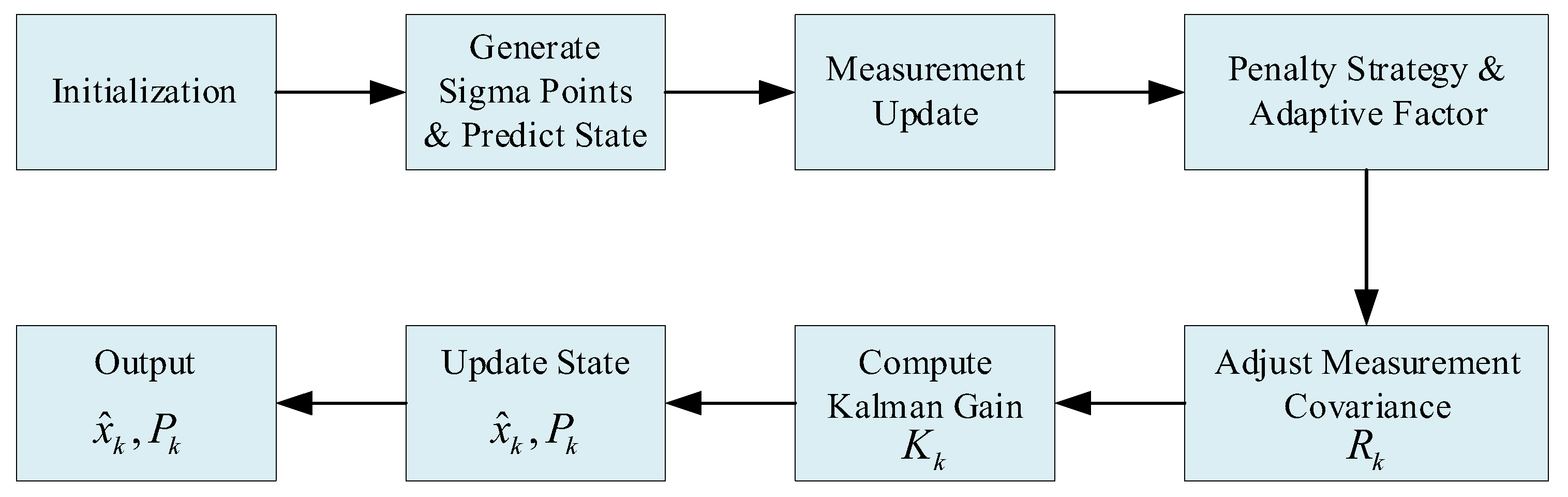
Article

Manoeuvring Surface Target Tracking in the Presence of Glint Noise Using the Robust Cubature Kalman Filter Based on the Current Statistical Model

1
Key Laboratory of High Performance Ship Technology, Wuhan University of Technology, Ministry of Education, #1178 Heping Road, Wuhan 430063, China
2
School of Naval Architecture, Ocean and Energy Power Engineering, Wuhan University of Technology, #1178 Heping Road, Wuhan 430063, China
3
Faculty of Civil Engineering and Geosciences, Delft University of Technology, Stevinweg, 1, 2628 CN Delft, The Netherlands
4
School of Navigation, Wuhan University of Technology, #1178 Heping Road, Wuhan 430063, China
*
Authors to whom correspondence should be addressed.
Electronics 2025, 14(10), 1973; https://doi.org/10.3390/electronics14101973
Submission received: 23 March 2025 / Revised: 27 April 2025 / Accepted: 8 May 2025 / Published: 12 May 2025
(This article belongs to the Special Issue Wind and Renewable Energy Generation and Integration)

Abstract

:
For manoeuvring surface target tracking in the presence of glint noise, Huber-based Kalman filters have been widely regarded as effective. However, when the proportion of outlier measurements is high, their numerical stability and estimation accuracy can deteriorate significantly. To address this issue, we propose a Robust Cubature Kalman Filter with the Current Statistical (RCKF_CS) model. Inspired by the Huber equivalent weight function, an adaptive factor incorporating a penalty strategy based on a smoothing approximation function is introduced to suppress the adverse effects of glint noise. The proposed method is then integrated into the Cubature Kalman Filter framework combined with the Current Statistical model. Unlike conventional Huber-based approaches, which process measurement residuals independently in each dimension, the proposed method evaluates the residuals jointly to improve robustness. Numerical stability analysis and extensive simulation experiments confirm that the proposed RCKF_CS achieves improved numerical robustness and filtering performance, even under strong glint noise conditions. Compared with existing Huber-based filters, the proposed method enhances filtering performance by 2.66% to 10.18% in manoeuvring surface target tracking tasks affected by glint noise.

1. Introduction

1.1. Research Background

In recent years, the increasing deployment of marine radar systems for ship navigation, port surveillance, and maritime safety has made the robust tracking of manoeuvring surface targets an essential capability. With the growing number of surface vehicles and the rising complexity of navigation environments, vessels are required to maintain high manoeuvrability to cope with various dynamic and uncertain conditions [1]. Marine radar technology plays a vital role in ensuring navigational safety by supporting real-time monitoring, collision avoidance, and search-and-rescue operations [2,3,4,5,6].
To meet these demands, signal processing techniques such as the Kalman filter [7] are widely adopted for target tracking. However, tracking performance can deteriorate significantly when the targets exhibit complex manoeuvres or the measurement is affected by glint noise, which introduces non-Gaussian characteristics into the radar signal and violates the assumptions of conventional filters.

1.2. Related Research

The Kalman filter, as the minimum-mean-square-error optimal linear estimator, is widely used in target tracking. Early works such as Singer and Stein proposed a linear Kalman filter for radar applications [8], with subsequent improvements like the Converted Measurement Kalman Filter (CMKF) designed to reduce coordinate transformation errors [9]. However, the CMKF shows poor convergence in manoeuvring scenarios, prompting the development of nonlinear alternatives including the Extended Kalman Filter (EKF) [10], Unscented Kalman Filter (UKF) [11], and Cubature Kalman Filter (CKF) [12]. Although EKF is widely adopted [13], it suffers from linearisation errors due to Jacobian computation. UKF improves upon EKF but is prone to filter collapse in high-dimensional systems [14]. In contrast, the CKF provides superior accuracy and numerical stability. Recent studies have further explored robust and adaptive variants of these filters to address dynamic tracking challenges [15,16].
The motion model of a manoeuvring target significantly affects filtering accuracy. Models such as the Singer model [8], the Jerk model [17], the Interacting Multiple Model (IMM) [18,19], and the Current Statistical (CS) model [20] have been developed to better capture target dynamics. The Singer model assumes zero-mean acceleration with uniform distribution, which may not align with real-world conditions. The Jerk model accounts for acceleration derivatives, improving tracking for highly manoeuvring targets at the cost of increased computational load. The IMM requires frequent updates to model transition probabilities and multiple sub-filters, further increasing complexity. In contrast, the CS model introduces a modified Rayleigh distribution to model acceleration changes, achieving a good balance between performance and computational efficiency. Recently, Yang et al. [21] proposed an improved multi-target tracking algorithm, termed Q-IMM-MHT. This method integrates Multiple Hypothesis Tracking (MHT) with IMM and introduces a Q-learning-based adaptive model switching strategy to dynamically adjust model selection in response to variations in the target’s motion patterns.
Nevertheless, these filters perform well only under Gaussian noise assumptions. In real radar tracking environments, signal reflections vary significantly due to random fluctuations in radar scattering intensity and phase across different parts of the target. As a result, the measurement noise becomes non-Gaussian, a phenomenon known as glint noise [22]. Glint noise is typically modelled using a mixture of Gaussian distributions as in [23,24,25], or a Gaussian–Laplacian mixture with zero mean as in [26]. Under such conditions, the performance of conventional filters is severely degraded.
To address this degradation, Zhou and Frank [27] proposed the Strong Tracking Filter (STF), which dynamically adjusts the error covariance matrix using residual-based attenuation factors. STF has been successfully applied in various filters [28,29], but it lacks robustness to outliers. In contrast, Huber’s robust estimation theory [30] effectively mitigates the impact of glint noise. Huber-based approaches leverage a piecewise loss function, combining the robustness of the least absolute deviation with the differentiability of least squares, yielding stable robust estimates. Charles et al. [31] introduced the Huber equivalent weight function into the Kalman filter framework, which was later extended to several nonlinear filters.
For example, Zhao et al. [32] developed a robust EKF based on the Huber function. Wang et al. [33] applied a Huber-based UKF to visual relative positioning. Yin et al. [34] proposed a derivative Unscented Kalman Filter, and Qiu and Guo [35] incorporated the Huber-based strategy into a strong tracking CKF to enhance robustness. Yu et al. [36] investigated the problems of robust adaptive Kalman filtering and smoothing for linear state-space models affected by heavy-tailed multiplicative measurement noise and additive process and measurement noises.
Although the above Huber-based filters exhibit promising performance, several key limitations remain: (1) these filters evaluate measurement residuals independently in each dimension, which can compromise numerical stability in multidimensional systems such as marine radar; and (2) for manoeuvring targets under glint noise, measurement residual variations are caused not only by outliers but also by rapid changes in target dynamics. In such cases, relying solely on fixed residual-based detection may misinterpret target motion as noise. Therefore, replacing the fixed-form Huber function with a more flexible adaptive strategy is desirable.

1.3. Contribution of This Work

In this study, a robust filtering approach is proposed to enhance tracking performance and numerical stability in multidimensional measurement systems such as marine radar, particularly under glint noise conditions. An adaptive factor based on a smooth approximation function [37] is introduced into the CKF with the CS model, yielding the robust CKF_CS. This design enhances the filter’s resilience to non-Gaussian measurement noise. Condition number analysis demonstrates that RCKF_CS offers superior numerical stability compared to Huber-based Kalman filters.
Extensive Monte Carlo simulations are conducted to compare the performance of RCKF_CS against CKF_CS, STCKF_CS, HCMKF_CS, HEKF_CS, HCKF_CS, and STHCKF_CS. The results indicate that RCKF_CS consistently achieves higher tracking accuracy for manoeuvring targets in the presence of glint noise.

1.4. Organisation

The remainder of this paper is organised as follows: The calculation process of the CS model and the CKF is reviewed in Section 2. The generation mechanism of glint noise and the analysis of the HCKF_CS are briefly explained in Section 3. The derivation of the RCKF_CS is presented in Section 4. The numerical stability analysis is presented in Section 5. The simulation experiment and result analysis are presented in Section 6. The conclusions are summarised in Section 7.

2. CKF_CS

2.1. CS Model

In the CS model, the motion equation and measurement equation are described as follows:
x k + 1 = F k x k + U k a ¯ k + ω k
z k + 1 = h x k + 1 + ν k + 1
where x k + 1 = x k + 1 x ˙ k + 1 x ¨ k + 1 T , x k + 1 , x ˙ k + 1 and x ¨ k + 1 are the position, velocity, and acceleration of the target, respectively. z k + 1 is the measurement vector. a ¯ k is the current acceleration mean. Process noise ω k follows a Gaussian distribution, and its covariance is Q k . Measurement noise ν k + 1 also follows a Gaussian distribution, and its covariance is R k + 1 . h · is the nonlinear mapping function. F k and U k are the state transition matrix and input control matrix, respectively. F k , U k , and Q k are described as follows:
F k = 1     T 1 + α T + e α T α 2 0     1 1 e α T α 0     0 e α T
U k = 1 α T + α T 2 2 + 1 e α T α T 1 e α T α 1 e α T
Q k = E ω k ω k T = 2 α σ α 2 q
where α is the manoeuvring frequency, T is the sampling interval, q is a constant matrix, and its expression can be found in [38].
Considering physical limitations, if a target is manoeuvring with a certain acceleration at present, then the region of acceleration in the next moment is limited and is around the “current” acceleration. Hence, it is supposed that the acceleration a k follows a modified Rayleigh distribution P r a k as follows:
P r a k = α m a x a ¯ k μ 2 e x p α m a x a ¯ k 2 2 μ 2 ,   0 a k α m a x
where α m a x is the maximum value of the acceleration, and σ α 2 is the acceleration variance, which can be obtained as follows:
σ α 2 = 4 π π α m a x a ¯ k 2
The CS model actually reflects the changes in the range and intensity of the manoeuvring target, so the filters using the CS model can provide good performance for manoeuvring target tracking.

2.2. CKF

The CKF can approximate the high-dimensional integral based on the spherical radial volume criterion, and its filtering process is described in Equations (8)–(22). Moreover, the notation k / k refers to the a posteriori estimate at time step k, while k + 1 / k denotes the one-step prediction for time k + 1 based on data available up to time k.
(1) 
Time update process
η j = n I n I n j
where I n is the identity matrix, and   ·   j represents the j-th column of the matrix, where j = 1,2 , , 2 n .
P k / k = S k / k S k / k T
χ j , k / k = S k / k η j + x ^ k / k
χ j , k + 1 / k = F χ j , k / k
x ^ k + 1 / k = j = 1 2 n w j χ j , k + 1 / k
P k + 1 / k = i = 1 2 n w j χ j , k + 1 / k χ j , k + 1 / k T x ^ k + 1 / k x ^ k + 1 / k T + Q k
where the weight of each measurement point in the CKF is equal, and w j = 1 / 2 n , j = 1,2 , , 2 n . Considering the CS model described in Section 2.1, Q k can be calculated by Equations (5) and (7).
(2) 
Measurement update process
P k + 1 / k = S k + 1 / k S k + 1 / k T
χ j , k + 1 / k * = S k + 1 / k η j + x ^ k + 1 / k
Z j , k + 1 / k = h χ j , k + 1 / k *
z ^ k + 1 / k = j = 1 2 n w j Z j , k + 1 / k
P x z , k + 1 / k = j = 1 2 n w j χ j , k + 1 / k x ^ k + 1 / k Z j , k + 1 / k z ^ k + 1 / k T
P z z , k + 1 / k = j = 1 2 n w j Z j , k + 1 / k Z j , k + 1 / k T z ^ k + 1 / k z ^ k + 1 / k T + R k + 1
Then, the filtering gain, state estimation, and covariance matrix are obtained as follows:
K k + 1 = P x z , k + 1 / k P z z , k + 1 / k 1
x ^ k + 1 / k + 1 = x ^ k + 1 / k + K k + 1 Z k + 1 z ^ k + 1 / k
P k + 1 / k + 1 = P k + 1 / k K k + 1 P z z , k + 1 / k K k + 1 T

3. HCKF_CS

It is well known that the Cubature Kalman Filter demonstrates excellent filtering performance when the measurement noise strictly follows a Gaussian distribution. However, its performance is significantly degraded when the noise deviates from this assumption. In real-world scenarios, due to the random variation in radar scattering intensity and phase across different parts of a target, the reflected radar signals often exhibit substantial fluctuations. As a result, the associated measurement noise deviates from the Gaussian model and exhibits non-Gaussian characteristics, typically referred to as glint noise.
To simulate glint noise, a Gaussian mixture distribution or a combination of Gaussian and Laplacian distributions is commonly employed, which can be mathematically expressed as follows:
G glint = ( 1 ε ) F 1 , N + ε F 2 , N
where F 1 , N is the main distribution of glint noise and follows a Gaussian distribution, F 2 , N is the pollution distribution of glint noise and follows a Gaussian distribution or Laplacian distribution with a large variance. The pollution rate of glint noise is ε 0 1 .
When the pollution rate of glint noise increases, the performance of CKF_CS deteriorates significantly. In contrast, the HCKF_CS can effectively address this problem. The main difference between the HCKF_CS and CKF_CS is that the covariance matrix of the measurement error is reconstructed as follows:
R k + 1 H C K F _ C S = R k + 1 1 / 2 ψ k + 1 1 R k + 1 T / 2
where ψ   = diag { ψ 1 , ψ 2 , , ψ m } is the robustness factor, and the equivalent weight function is calculated as follows:
ψ i = 1             , ζ i β β ζ i   , ζ i > β
where ψ i is the equivalent weight function. ζ i is the i-th dimension of the weighted residual vector ( R k + 1 1 / 2 Z k + 1 h ( x ^ k + 1 ) ). β is a threshold and is generally set to 1.345 [39]. Therefore, it can be concluded that the HCKF_CS handles each dimension of the weighted residual vector separately.

4. RCKF_CS with an Adaptive Factor

The variables and their corresponding symbols used in this section are shown in Table 1.
Inspired by a smoothing approximation function proposed by [37], f μ x = x 2 + μ 2 (where μ is a small positive constant approaching zero), an adaptive factor combined with a penalty strategy is introduced to mitigate the adverse effects of glint noise.
The nonlinear model is assumed as follows:
z k x ^ k / k 1 = h ( x k ) x k + v k δ x k / k 1
where δ x k / k 1 is the error between the extrapolated estimated value of the state and the true value. Its equation is described as follows:
δ x k / k 1 = x ^ k / k 1 x k
Let ε = v k δ x k / k 1 ; then,
E ( ε k ε k T ) = R k 0 m × n 0 n × m P k / k 1
Let S k = E ( ε k ε k T ) ; multiplying both sides of Equation (26) by S k 0.5 and defining the second term on the right side as ξ k , the following are obtained:
ξ k = R k 0 m × n 0 n × m P k / k 1 0.5 v k δ x k / k 1 = S k 0.5 v k δ x k / k 1
and
E ( ξ k ξ k T ) = I ( m + n ) + ( m + n )
The loss function at moment k is defined as follows:
J X k = ρ ξ k
where ρ ξ k is represented as
ρ ξ k =                 1 2 ξ k T ξ k ,                 ξ k T ξ k + μ 2 < γ ξ k T ξ k + μ 2 ,         ξ k T ξ k + μ 2 γ
Let ϕ k = ξ k T ξ k + μ 2 ; Equation (32) is simplified as follows:
ρ ξ k = ϕ k 2 μ 2 2 ,                     ϕ k < γ           ϕ k ,                               ϕ k γ
If Equation (29) is substituted into ϕ k , then ϕ k is reconstructed as follows:
ϕ k = ξ k T ξ k + μ 2 = S k 0.5 v k δ x k / k 1 T S k 0.5 v k δ x k / k 1 + μ 2 = v k δ x k / k 1 T S k 0.5 T S k 0.5 v k δ x k / k 1 + μ 2
That is,
ϕ k = v k T R k 1 v k + δ x k / k 1 T P k / k 1 1 δ x k / k 1 + μ 2
The optimal estimate can be obtained by minimising the loss function
x ^ k k = argmin ρ ξ k  
Equation (36) can be solved as follows:
φ ξ k ξ k x k = 0
where
φ ξ k = ξ k ,                             ϕ k < γ ξ k ξ k T ξ k + μ 2 ,         ϕ k γ
Let θ k = φ ξ k / ξ k ; then,
  θ k = 1 ,                     ϕ k < γ 1 ϕ k ,                 ϕ k γ
In Equation (27), the true value x k is not directly accessible; therefore, the extrapolated estimate x ^ k / k 1 is substituted into the equation. Consequently, the prediction error δ x k / k 1 is considered to be zero. The measurement noise v k is treated as the measurement residual, defined as e k = Z k z ^ k / k 1 .
Considering that μ approaches zero, let v k = e k ; therefore, Equation (35) is simplified as follows:
ϕ k = e k T R k 1 e k
where ϕ k is a nondimensional number constructed by the measurement residual.
The correction factor Θ is defined as follows:
Θ = θ k I m × m 0 m × n 0 m × n I n × n
Considering the correction factor in Equation (41), the measurement covariance matrix is reconstructed as S ~ k = S k 0.5 Θ 1 S k 0.5 T . Hence, S ~ k is simplified as follows:
S ~ k = S k 0.5 Θ 1 S k 0.5 T = λ k R k 0 m × n 0 m × n P k / k 1
where the adaptive factor with the penalty strategy λ k is defined as follows:
λ k = 1 ,                     ϕ k < γ ρ k ϕ k ,         ϕ k γ
where γ is a threshold, and ρ k represents the penalty strategy, which is defined as follows:
ρ k = η ,                                       exp ( ϕ k γ τ ) η exp ( ϕ k γ τ ) ,               exp ( ϕ k γ τ ) < η
where τ and η are two constant parameters. Equation (44) means an extra penalty for outliers that deviate far from the true value. In addition, as an upper threshold, η ensures that this penalty does not affect the observability of the filter.
According to the above calculation, the error covariance matrix of measurement is adjusted adaptively to effectively suppress the degradation of filtering performance. R k RCKF _ CS is defined as follows:
R k RCKF _ CS = λ k R k
Compared with CKF_CS, RCKF_CS converts Equation (19) into Equation (46):
P z z , k + 1 / k R C K F _ C S = j = 1 2 n w j Z j , k + 1 / k Z j , k + 1 / k T z ^ k + 1 / k z ^ k + 1 / k T + R k + 1 R C K F _ C S
The updating equations of RCKF_CS are obtained as follows:
K k + 1 RCKF _ CS = P x z , k + 1 / k ( P z z , k + 1 / k RCKF _ CS ) 1
x ^ k + 1 / k + 1 = x ^ k + 1 / k + K k + 1 R C K F _ C S Z k + 1 z ^ k + 1 / k
P k + 1 / k + 1 = P k + 1 / k K k + 1 R C K F _ C S P z z , k + 1 / k R C K F _ C S K k + 1 R C K F _ C S T
The RCKF_CS is composed of Equations (8)–(18) and Equations (46)–(49). Inspired by the idea of the Huber equivalent weight function, the proposed approach utilises the measurement residual comprehensively, and it uses adaptive factor λ k + 1 to change R k + 1 RCKF _ CS in time. The penalty strategy for adjusting the adaptive factor is constructed by the nondimensional number ϕ k + 1 . If there is a significant outlier in the measurement, λ k + 1 is promptly amplified to increase R k + 1 RCKF _ CS (by Equation (45)) and P z z , k + 1 / k RCKF _ CS (by Equation (46)), which will lessen the filtering gain K k + 1 RCKF _ CS (by Equation (47)). Then, the filtering performance can be improved by reducing the influence of the residual on state updating.
To better understand the logic and procedural flow of the proposed algorithm, Figure 1 provides a graphical illustration of the RCKF_CS steps, integrating the adaptive penalty strategy into the robust filtering framework.

5. Numerical Stability Analysis

For the CKF_CS, HCKF_CS, and RCKF_CS, the covariance matrices involved in the inverse calculation are described as follows:
P z z , k + 1 / k = j = 1 2 n w j Z j , k + 1 / k Z j , k + 1 / k T z ^ k + 1 / k z ^ k + 1 / k T + R k + 1
P z z , k + 1 / k HCKF _ CS = j = 1 2 n w j Z j , k + 1 / k Z j , k + 1 / k T z ^ k + 1 / k z ^ k + 1 / k T + R k + 1 HCKF _ CS
P z z , k + 1 / k RCKF _ CS = j = 1 2 n w j Z j , k + 1 / k Z j , k + 1 / k T z ^ k + 1 / k z ^ k + 1 / k T + R k + 1 RCKF _ CS
where R k + 1 H C K F _ C S = R k + 1 1 / 2 ψ k + 1 1 R k + 1 T / 2 , and R k + 1 RCKF _ CS = λ k + 1 R k + 1 . If the condition number of the covariance matrix on the left side of Equations (50)–(52) is too large, then the numerical stability of the filter will degrade. For the convenience of analysis, we describe the proof of Theorem 1 as follows:
Lemma 1.
For Hermite matrices R k + 1 1 / 2 and ψ z 1 / 2 of m × m , which have singular values σ 1 σ 2 . . . σ m 0 , there is
m i n r + s = i + 1 [ σ r ( R k + 1 1 / 2 ) σ s ( ψ z 1 / 2 ) ] σ i ( R k + 1 1 / 2 ψ z 1 / 2 ) m a x r + s = m + i [ σ r ( R k + 1 1 / 2 ) σ s ( ψ z 1 / 2 ) ] , i = 1 , . . . , m
Theorem 1.
If Hermite matrices R k + 1 1 / 2 and ψ z 1 / 2 meet
cond ( ψ z 1 / 2 ) cond ( R k + 1 )
where cond   ( ) = σ 1 / σ m   , which is defined as the condition number of the matrix.
Then,
cond ( R k + 1 HCKF _ CS ) cond ( R k + 1 RCKF _ CS )
Proof.
From Lemma 1, we have
σ 1 ( R k + 1 1 / 2 ψ z 1 / 2 ) σ m ( R k + 1 1 / 2 ) σ 1 ( ψ z 1 / 2 )
σ 1 ( R k + 1 1 / 2 ) σ m ( ψ z 1 / 2 ) σ m ( R k + 1 1 / 2 ψ z 1 / 2 )
If Equation (54) holds, then
cond ( ψ z 1 / 2 ) cond ( R k + 1 1 / 2 )
Therefore, there is
σ m ( R k + 1 1 / 2 ) σ 1 ( ψ z 1 / 2 ) σ 1 ( R k + 1 1 / 2 ) σ m ( ψ z 1 / 2 )
From Equations (56)–(59), we have
σ 1 ( R k + 1 1 / 2 ψ z 1 / 2 ) σ m ( R k + 1 1 / 2 ) σ 1 ( ψ z 1 / 2 ) σ 1 ( R k + 1 1 / 2 ) σ m ( ψ z 1 / 2 ) σ m ( R k + 1 1 / 2 ψ z 1 / 2 )
Then,
c o n d ( R k + 1 1 / 2 ψ z 1 / 2 ) = σ 1 ( R k + 1 1 / 2 ψ z 1 / 2 ) σ m ( R k + 1 1 / 2 ψ z 1 / 2 ) σ m ( R k + 1 1 / 2 ) σ 1 ( ψ z 1 / 2 ) σ 1 ( R k + 1 1 / 2 ) σ m ( ψ z 1 / 2 ) = c o n d ( ψ z 1 / 2 ) c o n d ( R k + 1 1 / 2 )
Considering
cond ( R k + 1 ) = [ cond ( R k + 1 1 / 2 ) ] 2
Equation (62) is substituted into Equation (54); then,
cond ( ψ z 1 / 2 ) [ cond ( R k + 1 1 / 2 ) ] 2
Equation (63) is substituted into Equation (61); then,
cond ( R k + 1 1 / 2 ψ z 1 / 2 ) cond ( R k + 1 1 / 2 )
Considering
cond ( R k + 1 1 / 2 ψ z 1 R k + 1 T / 2 ) = cond ( R k + 1 1 / 2 ψ z 1 / 2 ) 2
Then,
cond ( R k + 1 1 / 2 ψ z 1 R k + 1 T / 2 ) cond ( R k + 1 )
Noting cond ( R k + 1 HCKF ) = cond ( R k + 1 1 / 2 ψ z 1 R k + 1 T / 2 ) , and cond ( R k + 1 RCKF ) = cond ( λ k + 1 R k + 1 ) = cond ( R k + 1 ) , then Equation (55) holds.
From Equation (25), it is known that ψ is the result of handling each dimension of the residual vector separately. Therefore, the condition number of ψ becomes extremely large if the measurement error of one dimension is significantly greater than the measurement error of other dimensions. In this situation, it is easy to meet Equation (54), and then Equation (55) holds according to Theorem 1. Moreover, under glint noise with a high pollution rate, λ k + 1 in Equation (44) will be relatively larger, so that on the right side of Equation (52), R k + 1 RCKF _ CS will be much greater than in other parts. Then, cond ( P z z , k + 1 / k RCKF _ CS ) is sufficiently close to cond ( R k + 1 RCKF _ CS ) . Similarly, under glint noise with a high pollution rate, cond ( P z z , k + 1 / k HCKF _ CS ) is also sufficiently close to cond ( R k + 1 HCKF _ CS ) . Therefore, according to Theorem 1, it is more likely that cond ( P z z , k + 1 / k HCKF _ CS ) is larger than cond ( P z z , k + 1 / k RCKF _ CS ) . The above analysis shows that although the Huber-based approach can achieve good filtering performance, it sacrifices numerical stability. However, the RCKF_CS achieves superior filtering performance with less loss of numerical stability; this can be verified by simulation experiments.
It is noted that the penalty strategy described by Equation (44) is not suitable for the Huber-based approach. Otherwise, cond ( P z z , k + 1 / k HCKF _ CS ) becomes greater such that the numerical stability of the Huber-based approach becomes much worse. □

6. Simulation and Analysis

To evaluate the performance and robustness of the proposed RCKF_CS algorithm under diverse tracking scenarios and glint noise conditions, a comprehensive set of simulations is conducted. While the complete results are included for the sake of transparency and reproducibility, key representative cases are highlighted in the text and figure captions to guide the reader’s attention.
For clarity, the simulation analysis is organised into three aspects: method comparison, noise-level sensitivity, and numerical stability evaluation.

6.1. Simulation Conditions

For different surface tracks, Monte Carlo simulation experiments are used to compare CKF_CS, STCKF_CS, HCMKF_CS, HEKF_CS, HCKF_CS, STHCKF_CS and RCKF_CS. The number of simulations (M) is 200. It is assumed that the standard deviation of radar range noise is 50 m, and the standard deviation of angle noise is 0.5°. The radar sampling time is 1000 s, and the sampling interval is 0.1 s. The simulations are implemented based on Python 3.8. The hardware configuration of the experiment is as follows: the CPU is an AMD Ryzen 5 2600 (Advanced Micro Devices, Santa Clara, CA, USA; clock speed at 3.4 GHz), with 8G of memory, and a 512G solid-state disc, without CPU overclocking and multithreading technology.
For the baseline filters HCMKF_CS and HEKF_CS, the threshold parameter β in the Huber function was set to 1.345, following the recommendation by [39], which is commonly adopted in the robust estimation literature. This choice ensures fair and consistent comparison with the proposed method.
The four surface tracks are designed under different manoeuvring states. The surface tracks are shown in Figure 2, and the speed distribution of each surface track is shown in Figure 3.
The measurement noise v k is simulated by glint noise, which follows the distribution below:
p v k = ( 1 ε ) N 0 , D 1 + ε B 0 , D 2
where N 0 , D 1 is the main distribution, B 0 , D 2 is the pollution distribution, and D 2 = 50 D 1 .
According to the different types of pollution distribution, the experiments can be divided into Experiment A and Experiment B. B 0 , D 2 in Experiment A follows Gaussian distribution, while B 0 , D 2 in Experiment B follows Laplacian distribution.
To verify the tracking performance of each filter for manoeuvring surface targets in the presence of glint noise, three examples were designed using different pollution rates under each track. The pollution rate ε of these three examples are set to 0.1, 0.2, and 0.4. If ε is greater than or equal to 0.1, then it is considered to be a high pollution rate. For the two types of pollution distributions, the logarithmic curves of the Probability Density Function (PDF) of glint noise under different pollution rates are shown in Figure 4 and Figure 5. From Figure 4 and Figure 5, it is indicated that the glint noise of Experiment A or B has obvious heavy-tailed statistical characteristics.
Other conditions in this paper are described as follows: acceleration maximum value of the CS model a m a x = 0.1 m/s2.
As a summary of the above, the important simulation conditions are listed in Table 2.

6.2. Comparison of the Parameter Settings of the Adaptive Factor with the Penalty Strategy

The relative performance of the different parameter settings of the adaptive factor with the penalty strategy (described in Equations (43) and (44)) is compared through the following simple experiments. In the experiments, 24 examples are used to test 8 groups of parameter combinations as shown in Table 3. The test results are presented in Table 4 and Table 5. The first column shows the track number and pollution rate ε, and Columns 2–9 report the mean values of the RMSE of RCKF_CS (time period of 200~1000 s) for the different parameter combinations.
As shown in Table 4 and Table 5, the parameter combinations P1 and P3 outperformed the other parameter combinations, and P1 is better than P3. Thus, P1 is chosen as the standard parameter setting of the adaptive factor with the penalty strategy which can obtain better filtering performance. Therefore, the constant parameters related to the adaptive factor are set to η = 10 , τ = 100 , and γ = 4.25 .
To ensure the effectiveness of the adaptive factor, a structured experimental tuning approach was adopted. Specifically, eight combinations of the parameters η , τ , γ were tested (as shown in Table 3), and the optimal set (P1: η = 10 , τ = 100 , γ = 4.25 ) was selected based on the lowest average RMSE across multiple simulation tracks and noise levels.

6.3. Results and Analysis

The Root Mean Square Error (RMSE) of the position and condition number ratio are, respectively, described as follows:
RMSE = 1 M i = 1 M ( x ^ i x i ) 2 1 2
CR = lg cond ( P z z HCKF _ C S ) / cond ( P z z RCKF _ CS )
For Experiment A, Figure 6, Figure 7, Figure 8, Figure 9, Figure 10, Figure 11, Figure 12, Figure 13, Figure 14, Figure 15, Figure 16 and Figure 17 show the RMSE of the position, and Figure 18, Figure 19, Figure 20 and Figure 21 show the CR under the different pollution rates. To reveal the filtering performance of each filter more accurately, Table 6, Table 7, Table 8 and Table 9 show the average RMSE of each filter in the time period from 200 to 1000 s.
For Experiment B, Figure 22, Figure 23, Figure 24, Figure 25, Figure 26, Figure 27, Figure 28, Figure 29, Figure 30, Figure 31, Figure 32, Figure 33, Figure 34, Figure 35, Figure 36 and Figure 37 show the RMSE of the position and the CR. Moreover, Table 10, Table 11, Table 12 and Table 13 show the average RMSE of each filter in the time period from 200 to 1000 s.
From these experimental results, the following can be observed:
(1)
As shown in Figure 6, Figure 7, Figure 8, Figure 9, Figure 10, Figure 11, Figure 12, Figure 13, Figure 14, Figure 15, Figure 16, Figure 17, Figure 18, Figure 19, Figure 20 and Figure 21, CKF_CS and STCKF_CS demonstrate serious performance degradation even if there is glint noise in the minor manoeuvring case. This indicates that they cannot suppress the negative influence caused by glint noise.
(2)
HCMKF_CS and HEKF_CS rapidly deteriorates with increasing pollution rate or acceleration according to Figure 6, Figure 7, Figure 8, Figure 9, Figure 10, Figure 11, Figure 12, Figure 13, Figure 14, Figure 15, Figure 16 and Figure 17 and Figure 22, Figure 23, Figure 24, Figure 25, Figure 26, Figure 27, Figure 28, Figure 29, Figure 30, Figure 31, Figure 32 and Figure 33. Moreover, their RMSE soars whenever the target manoeuvring states abruptly change. Hence, their filtering performance is far inferior to the filtering performance of the other three types of robust approaches.
(3)
In light of Figure 6, Figure 7, Figure 8, Figure 9, Figure 10, Figure 11, Figure 12, Figure 13, Figure 14, Figure 15, Figure 16 and Figure 17 and Table 6, Table 7, Table 8 and Table 9, the superiority of RCKF_CS to HCKF_ CS or STHCKF_CS is generally evident under any pollution rate for the same track. Furthermore, in comparison to the RCKF_CS, the RMSE of the HCKF_CS or STHCKF_CS clearly increases as the target manoeuvring from track 1~4 gradually increases at the same pollution rate. Similarly, as observed from Figure 22, Figure 23, Figure 24, Figure 25, Figure 26, Figure 27, Figure 28, Figure 29, Figure 30, Figure 31, Figure 32 and Figure 33 and Table 10, Table 11, Table 12 and Table 13, the above analyses still hold if the pollution distribution of glint noise is a Laplacian distribution. Therefore, it is shown that RCKF_CS demonstrates better adaptability for manoeuvring target tracking under glint noise than the two Huber-based approaches.
(4)
From the analysis of Table 6, Table 7, Table 8, Table 9, Table 10, Table 11, Table 12 and Table 13, the average RMSE of RCKF_CS is the smallest when the pollution rate increases. The average RMSE of RCKF_CS is also the smallest when acceleration increases gradually. This shows that the RCKF_CS outperforms the other robust approaches in terms of filtering performance.
(5)
As observed from Figure 18, Figure 19, Figure 20 and Figure 21, under any pollution rate or in any manoeuvring state, the condition number of HCKF_CS is always larger than that of the RCKF_CS. This result is consistent with the theoretical analysis in Section 5. The condition number ratio between P z z HCKF _ CS and P z z RCKF _ CS gradually increases when the pollution rate rises, which means that the condition number of HCKF_CS gradually becomes larger in comparison to that of RCKF_CS. This indicates that an increase in the pollution rate can lead to a significant decline in the numerical stability of HCKF_CS. Similarly, it can be observed from Figure 34, Figure 35, Figure 36 and Figure 37 that the above analyses still hold in Experiment B. In fact, the Huber-based approaches improve the robustness at the expense of the decline in numerical stability. Moreover, this situation becomes serious as the pollution rate increases. Notably, the condition number analysis of this paper is also applicable to the comparison between the other Huber-based filters and RCKF_CS.
In summary, across all scenarios tested, the proposed RCKF_CS consistently demonstrated superior tracking accuracy, especially under non-Gaussian glint noise. It outperformed classical filters (CKF_CS, HCKF_CS) and also showed better numerical stability compared to Huber-based methods. These findings confirm the robustness and effectiveness of the adaptive penalty strategy integrated in RCKF_CS.

7. Conclusions

For manoeuvring surface target tracking, the filtering performance of conventional filters tends to degrade significantly in the presence of glint noise. Although Huber-based filters can enhance robustness, they often do so at the expense of numerical stability, especially under high noise contamination rates. In this paper, a RCKF_CS is proposed to address these challenges. Through both theoretical analysis and comprehensive simulation experiments, it is demonstrated that RCKF_CS not only offers improved numerical stability, but also achieves superior filtering performance compared to existing methods. The analysis in Section 5 shows that the degradation of numerical stability in Huber-based filters arises from treating measurement residuals independently in each dimension, a limitation that is particularly problematic in multidimensional measurement systems such as marine radar. In this context, RCKF_CS demonstrates clear advantages. However, it should be noted that for one-dimensional tracking problems, this issue does not arise, and therefore, the proposed approach may not offer substantial benefits over existing Huber-based filters in such cases.
Furthermore, certain limitations of the proposed method merit attention. The performance of RCKF_CS may degrade when tracking targets with extremely abrupt or discontinuous manoeuvres, where the underlying motion model becomes less valid. In addition, although our simulations demonstrate strong numerical stability in a radar-based system, further validation is needed in real-time, high-dimensional sensor fusion scenarios. These aspects represent important directions for future work. In follow-up research, the proposed adaptive factor and penalty strategy could be embedded into multiple-model frameworks such as the IMM or extended to particle filter architectures to evaluate their generalizability. Moreover, applying RCKF_CS to broader real-world applications may further demonstrate its practical value and robustness.

Author Contributions

Y.G.: Writing—original draft, Software, Methodology, Conceptualization; T.Y.: Writing—original draft; J.T.: Writing—review & editing; J.M.: Funding acquisition; B.W.: Writing—review & editing; Supervision; Visualization. All authors have read and agreed to the published version of the manuscript.

Funding

This study was funded by the National Natural Science Foundation of China (52271367).

Institutional Review Board Statement

This article does not contain any studies with human participants or animals performed by any of the authors.

Data Availability Statement

Data generated or analysed during the study are available from the corresponding author by request.

Acknowledgments

The authors would like to thank all the reviewers for their constructive comments. This work was supported by the National Natural Science Foundation of China (Project No.: 52271367).

Conflicts of Interest

The authors declare that they have no conflicts of interest.

Abbreviations

AcronymFull Term
CKFCubature Kalman Filter
CKF_CSCubature Kalman Filter with Current Statistical model
RCKF_CSRobust Cubature Kalman Filter with Current Statistical model
HCKF_CSStrong Tracking Cubature Kalman Filter with Current Statistical model
STCKF_CSStrong Tracking Cubature Kalman Filter with Current Statistical model
HCMKF_CSHuber-based Cubature Modified Kalman Filter with Current Statistical model
HEKF_CSHuber-based Extended Kalman Filter with Current Statistical model
STHCKF_CSStrong Tracking Huber-based Cubature Kalman Filter with Current Statistical model
RMSRoot Mean Square
RMSERoot Mean Square Error
IMMInteracting Multiple Model
PDFProbability Density Function
SNRSignal-to-Noise Ratio

References

  1. Bilik, I.; Tabrikian, J. Manoeuvring target tracking in the presence of glint using the nonlinear gaussian mixture kalman filter. IEEE Trans. Aerosp. Electron. Syst. 2010, 46, 246–262. [Google Scholar] [CrossRef]
  2. Kumar, M.; Mondal, S. Recent developments on target tracking problems: A review. Ocean. Eng. 2021, 236, 109558. [Google Scholar] [CrossRef]
  3. Sinisterra, A.J.; Dhanak, M.R.; Ellenrieder, K.V. Stereovision-based target tracking system for USV operations. Ocean Eng. 2017, 133, 197–214. [Google Scholar] [CrossRef]
  4. Benetazzo, A.; Serafino, F.; Bergamasco, F.; Ludeno, G.; Ardhuin, F.; Sutherland, P.; Sclavo, M.; Barbariol, F. Stereo imaging and X-band radar wave data fusion: An assessment. Ocean. Eng. 2018, 152, 346–352. [Google Scholar] [CrossRef]
  5. Zhou, Y.; Wang, T.; Hu, R.H.; Su, H.; Liu, Y.; Liu, X.M.; Suo, J.D.; Snoussi, H. Multiple Kernelized Correlation Filters (MKCF) for Extended Object Tracking Using X-Band Marine Radar Date. IEEE Trans. Signal Process. 2019, 67, 3676–3688. [Google Scholar] [CrossRef]
  6. Leclerc, M.; Tharmarasa, R.; Florea, M.C.; Boury-Brisset, A.-C.; Kirubarajan, T.; Duclos-Hindié, N. Ship classification using deep learning techniques for maritime target tracking. In Proceedings of the 2018 21st International Conference on Information Fusion (FUSION), Cambridge, UK, 10–13 July 2018; pp. 737–744. [Google Scholar]
  7. Kalman, R.E. A new approach to linear filtering and prediction problems. J. Basic Eng. 1960, 82, 35–45. [Google Scholar] [CrossRef]
  8. Singer, R.A.; Stein, J.J. An optimal tracking filter for processing sensor data of imprecisely determined origin in surveillance systems. In Proceedings of the 1971 IEEE Conference on Decision and Control, Miami Beach, FL, USA, 15–17 December 1971; pp. 171–175. [Google Scholar] [CrossRef]
  9. Lerro, D.; Bar-Shalom, Y. Tracking with debiased consistent converted measurements versus EKF. IEEE Trans. Aerosp. Electron. Syst. 1993, 29, 1015–1022. [Google Scholar] [CrossRef]
  10. Masazade, E.; Fard Ad, M.; Varshney, P.K. Sparsity-promoting extended kalman filtering for target tracking in wireless sensor networks. IEEE Signal Process. Lett. 2012, 19, 845–848. [Google Scholar] [CrossRef]
  11. Julier, S.J.; Uhlmann, J.K. Unscented filtering and nonlinear estimation. Proc. IEEE 2004, 92, 401–422. [Google Scholar] [CrossRef]
  12. Arasaratnam, I.; Haykin, S. Cubature kalman filters. IEEE Trans. Autom. Control. 2009, 54, 1254–1269. [Google Scholar] [CrossRef]
  13. Sabet, M.T.; Fathi, A.R.; Mohammadi Daniali, H.R. Optimal design of the Own Ship maneuver in the bearing-only target motion analysis problem using a heuristically supervised Extended Kalman Filter. Ocean Eng. 2016, 123, 146–153. [Google Scholar] [CrossRef]
  14. Jondhale, S.R.; Deshpande, R.S. Kalman Filtering Framework-Based Real Time Target Tracking in Wireless Sensor Networks Using Generalized Regression Neural Networks. IEEE Sens. J. 2019, 19, 224–233. [Google Scholar] [CrossRef]
  15. Yu, Y.F.; Chen, Z.S.; Zhang, Y.; Zhang, C.B.; Ding, W.P. Learning Dynamic-Sensitivity Enhanced Correlation Filter with Adaptive Second-Order Difference Spatial Regularization for UAV Tracking. IEEE Trans. Intell. Transp. Syst. (Early Access) 2025, 26, 1–20. [Google Scholar] [CrossRef]
  16. Liang, Y.; Xiong, L.; Shan, Y.; Wang, H. Learning Multi-Task Target-Specific Correlation Filters for Robust Tracking. IEEE Trans. Circuits Syst. Video Technol. (Early Access) 2025, 1. [Google Scholar] [CrossRef]
  17. Mehrotra, K.; Mahapatra, P.R. A jerk model for tracking highly manoeuvring targets. IEEE Trans. Aerosp. Electron. Syst. 1997, 33, 1094–1105. [Google Scholar] [CrossRef]
  18. Magill, D. Optimal adaptive estimation of sampled stochastic processes. IEEE Trans. Autom. Control 1965, 10, 434–439. [Google Scholar] [CrossRef]
  19. Song, R.; Chen, X.; Fang, Y.; Huang, H. Integrated navigation of GPS/INS based on fusion of recursive maximum likelihood IMM and Square-root Cubature Kalman filter. ISA Trans. 2020, 105, 387–395. [Google Scholar] [CrossRef]
  20. Kumar, K.; Zhou, H.R. A ‘current’ statistical model and adaptive algorithm for estimating manoeuvring targets. J. Guid. Control Dyn. 1984, 7, 596–602. [Google Scholar] [CrossRef]
  21. Yang, Z.; Nie, H.; Liu, Y.; Bian, C. Robust Tracking Method for Small Weak Multiple Targets Under Dynamic Interference Based on Q-IMM-MHT. Sensors 2025, 25, 1058. [Google Scholar] [CrossRef]
  22. Hewer, G.A.; Martin, R.D.; Zeh, J. Robust preprocessing for Kalman filtering of glint noise. IEEE Trans. Aerosp. Electron. Syst. 2016, 23, 120–128. [Google Scholar] [CrossRef]
  23. Kulikov, G.Y.; Kulikova, M.V. Square-root accurate continuous-discrete extended-unscented kalman filtering methods with embedded orthogonal and j-orthogonal qr decompositions for estimation of nonlinear continuous-time stochastic models in radar tracking. Signal Process. 2020, 166, 107253.1–107253.15. [Google Scholar] [CrossRef]
  24. Liu, H.; Wu, W. Strong tracking spherical simplex-radial cubature kalman filter for manoeuvring target tracking. Sensors 2017, 17, 741. [Google Scholar] [CrossRef]
  25. Wu, W.R. Target tracking with glint noise. IEEE Trans. Aerosp. Electron. Syst. 1993, 29, 174–185. [Google Scholar] [CrossRef]
  26. Wu, W.R.; Cheng, P.P. A nonlinear IMM algorithm for manoeuvring target tracking. IEEE Trans. Aerosp. Electron. Syst. 1994, 30, 875–886. [Google Scholar] [CrossRef]
  27. Zhou, D.H.; Frank, P.M. Strong tracking kalman filtering of nonlinear time-varying stochastic systems with coloured noise: Application to parameter estimation and empirical robustness analysis. Int. J. Control 1996, 65, 295–307. [Google Scholar] [CrossRef]
  28. He, Y.; Qiang, S.; Dong, Y.L.; Yang, J. Adaptive Tracking Algorithm Based on Modified Strong Tracking Filter. In Proceedings of the 2006 CIE International Conference on Radar, Shanghai, China, 16–19 October 2006; Available online: https://www.webofscience.com/wos/alldb/fullrecord/WOS:000244659500459 (accessed on 7 May 2025).
  29. Huang, Y.; Zhang, Y.; Shi, P.; Wu, Z.; Qian, J.; Chambers, J.A. Robust kalman filters based on gaussian scale mixture distributions with application to target tracking. IEEE Trans. Syst. Man Cybern. Syst. 2017, 49, 2082–2096. [Google Scholar] [CrossRef]
  30. Huber, P.J. Robust Estimation of a Location Parameter. Ann. Math. Stat. 1964, 35, 73–101. [Google Scholar] [CrossRef]
  31. Boncelet, C.G.; Dickinson, B.W. An approach to robust Kalman filtering. In Proceedings of the 22nd IEEE Conference on Decision and Control, San Antonio, TX, USA, 14–16 December 1983; pp. 304–305. [Google Scholar] [CrossRef]
  32. Zhao, J.; Netto, M.; Mili, L. A robust iterated extended kalman filter for power system dynamic state estimation. IEEE Trans. Power Syst. 2017, 32, 3205–3216. [Google Scholar] [CrossRef]
  33. Wang, X.; Cui, N.; Guo, J. Huber-based unscented filtering and its application to vision-based relative navigation. Radar Sonar Navig. IET 2010, 4, 134–141. [Google Scholar] [CrossRef]
  34. Yin, L.J.; Deng, Z.H.; Huo, B.Y.; Xia, Y.Q.; Li, C. Robust Derivative Unscented Kalman Filter Under Non-Gaussian Noise. IEEE Access 2018, 6, 33129–33135. [Google Scholar] [CrossRef]
  35. Qiu, Z.; Guo, L. Improved cubature kalman filter for spacecraft attitude estimation. IEEE Trans. Instrum. Meas. 2021, 7, 1–13. [Google Scholar] [CrossRef]
  36. Yu, X.; Qu, Z.; Jin, G. Robust Adaptive Filters and Smoothers for Linear Systems with Heavy-Tailed Multiplicative/Additive Noises. IEEE Trans. Aerosp. Electron. Syst. 2024, 60, 6717–6733. [Google Scholar] [CrossRef]
  37. Caccetta, L.; Qu, B.; Zhou, G. A globally and quadratically convergent method for absolute value equations. Comput. Optim. Applications. 2011, 48, 45–58. [Google Scholar] [CrossRef]
  38. Singer, R.A. Estimating optimal tracking filter performance for manned manoeuvring targets. IEEE Trans. Aerosp. Electron. Syst. 1970, 6, 473–483. [Google Scholar] [CrossRef]
  39. Karlgaard, C.; Schauby, H. Comparison of Several Nonlinear Filters for a Benchmark Tracking Problem. In Proceedings of the AIAA Guidance, Navigation, and Control Conference and Exhibit, Chicago, IL, USA, 21–24 August 2006; p. 6243. [Google Scholar] [CrossRef]
Figure 1. Flowchart of the proposed RCKF_CS algorithm illustrating the key steps.
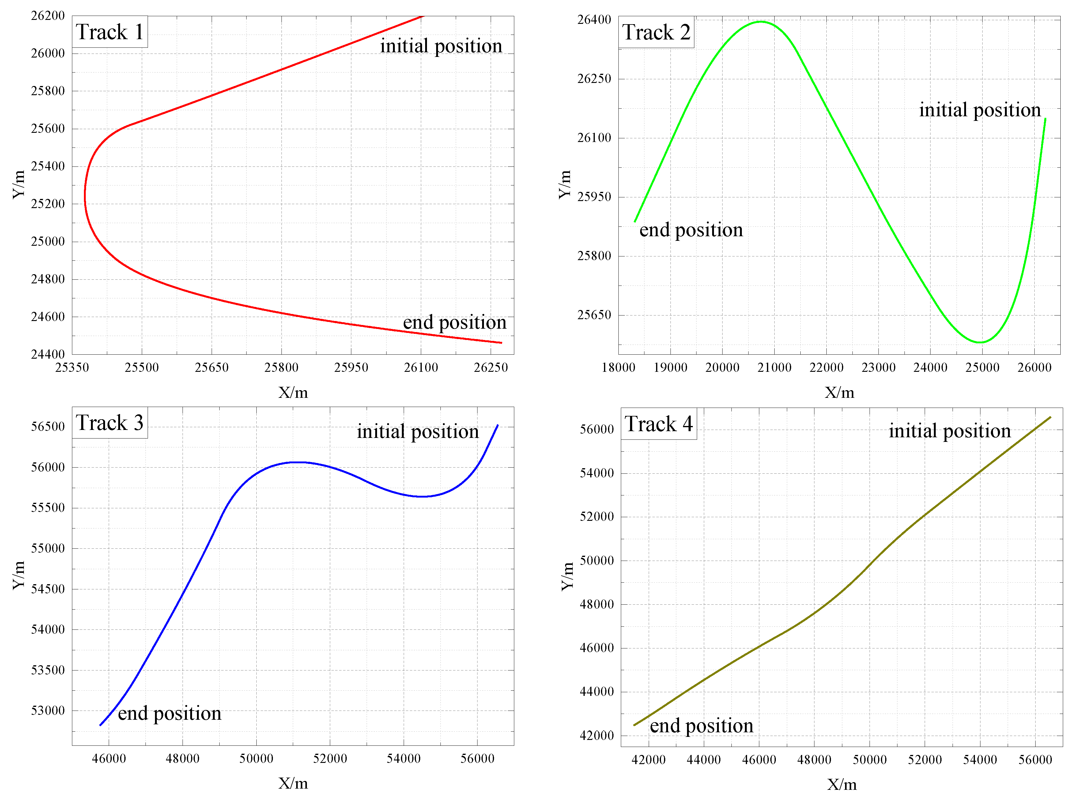
Electronics 14 01973 g001
Figure 2. Surface tracks.
Electronics 14 01973 g002
Figure 3. Velocity distribution of 4 surface tracks.
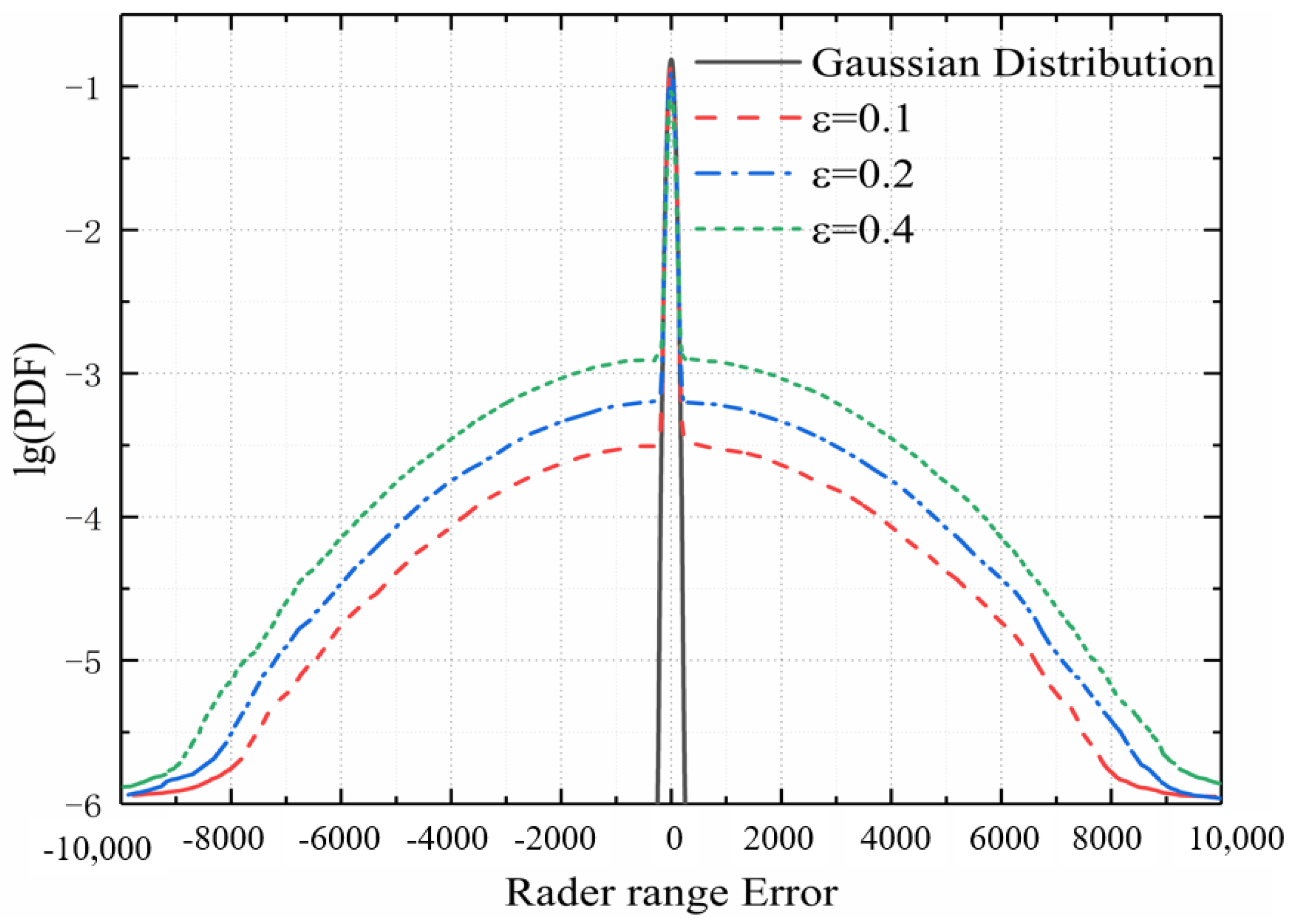
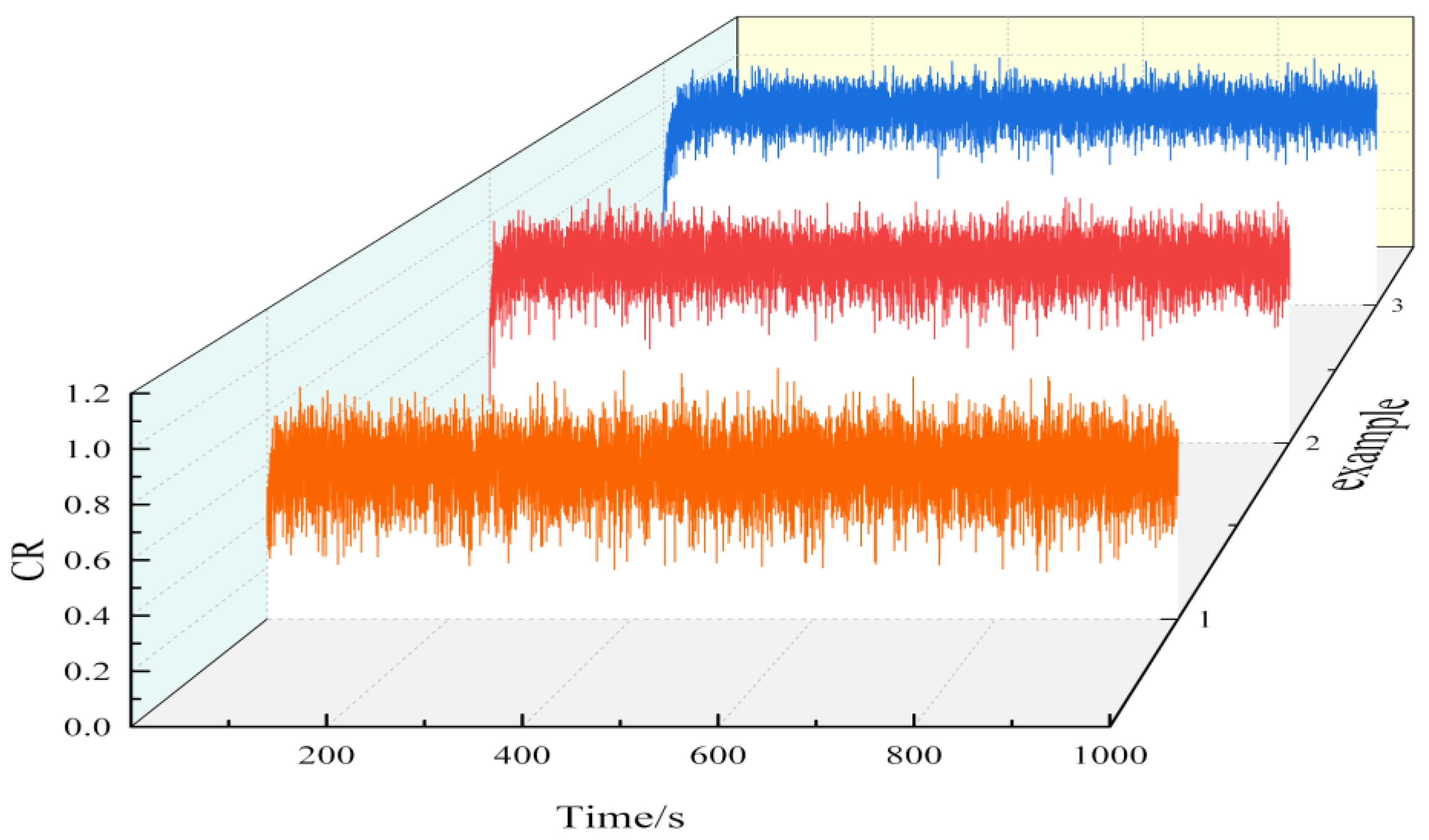
Electronics 14 01973 g003
Figure 4. The lg (PDF) of glint noise of Experiment A.
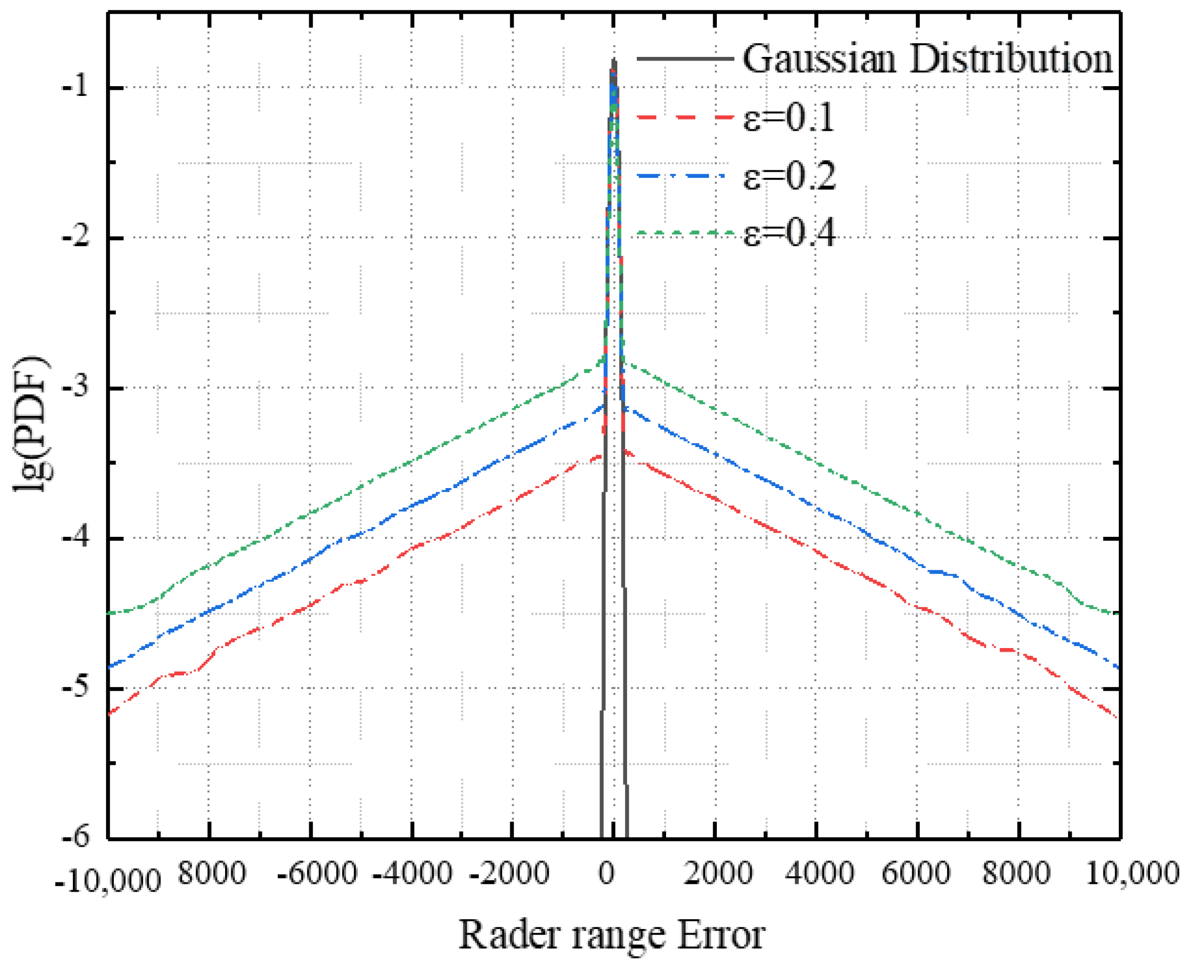
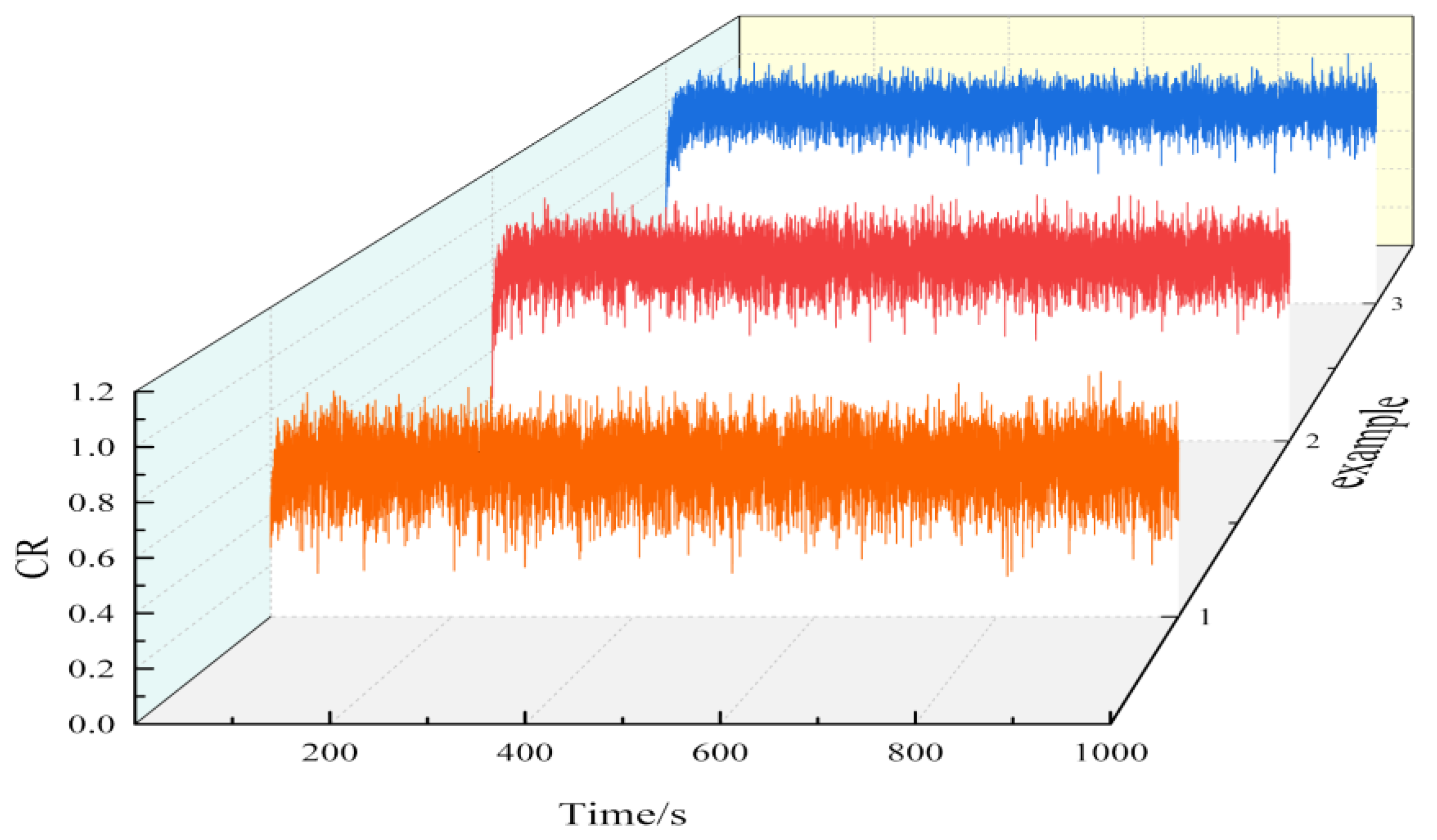
Electronics 14 01973 g004
Figure 5. The lg (PDF) of glint noise of Experiment B.
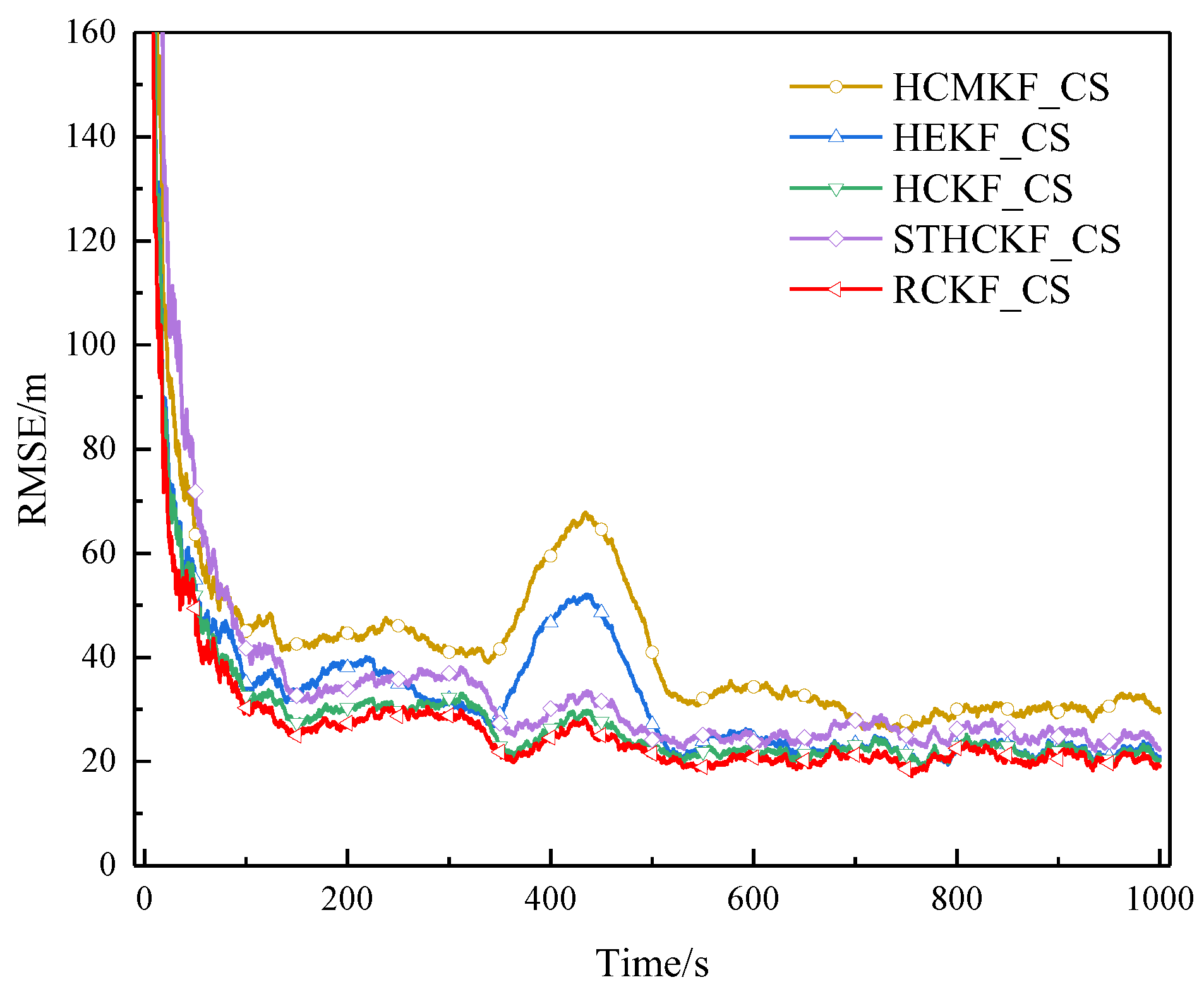
Electronics 14 01973 g005
Figure 6. RMSE of example 1 in surface track 1 (Experiment A).
Electronics 14 01973 g006
Figure 7. RMSE of example 2 in surface track 1 (Experiment A).
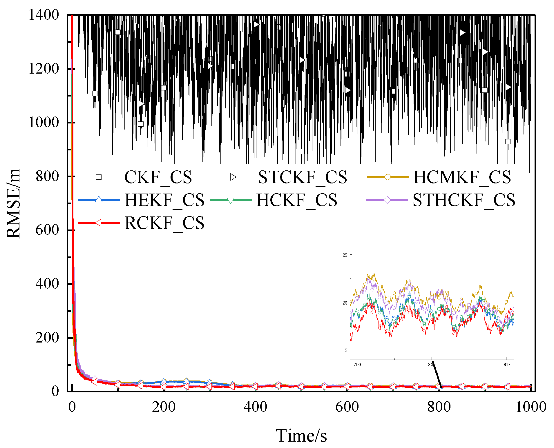
Electronics 14 01973 g007
Figure 8. RMSE of example 3 in surface track 1 (Experiment A).
Electronics 14 01973 g008
Figure 9. RMSE of example 1 in surface track 2 (Experiment A).
Electronics 14 01973 g009
Figure 10. RMSE of example 2 in surface track 2 (Experiment A).
Electronics 14 01973 g010
Figure 11. RMSE of example 3 in surface track 2 (Experiment A).
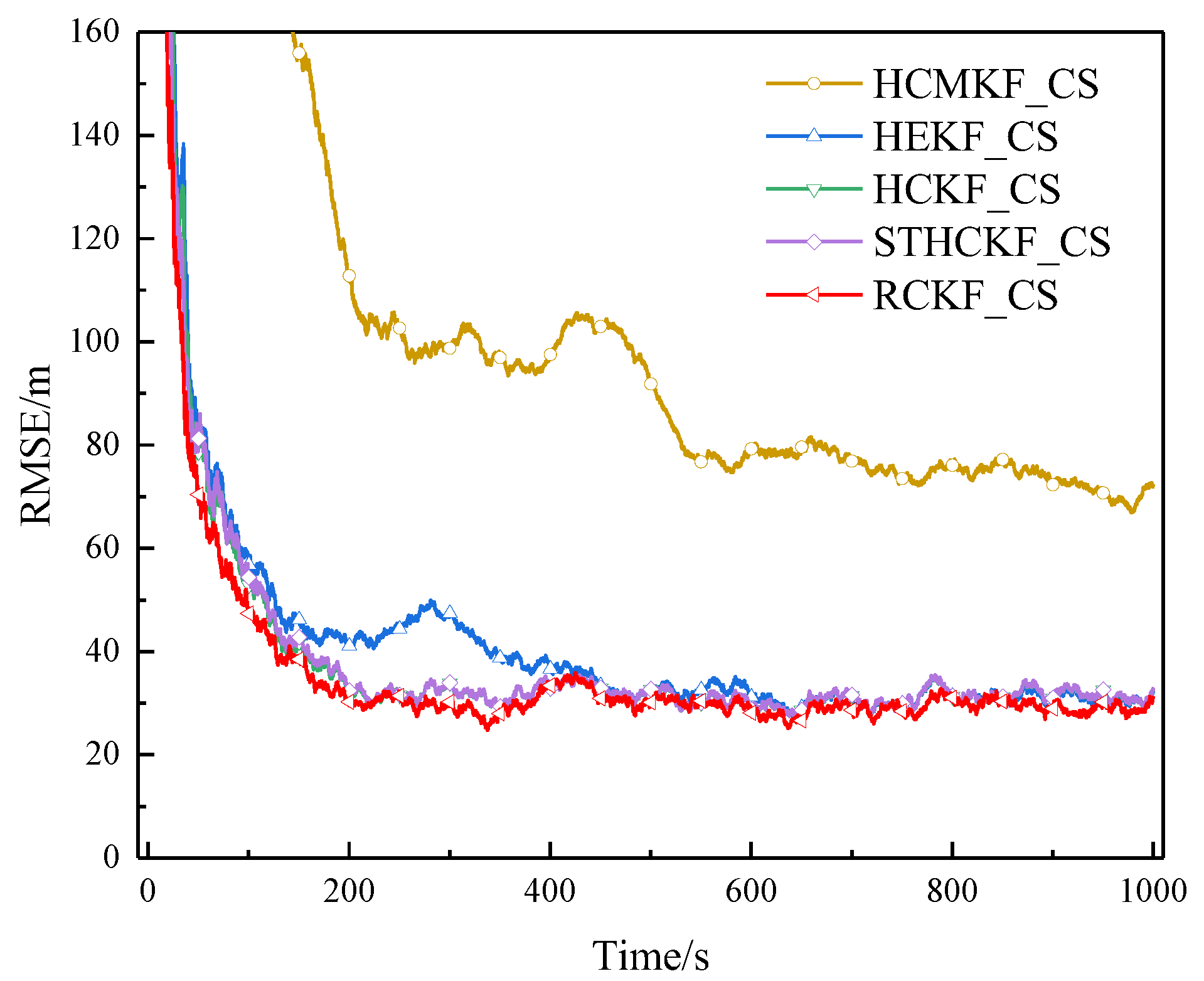
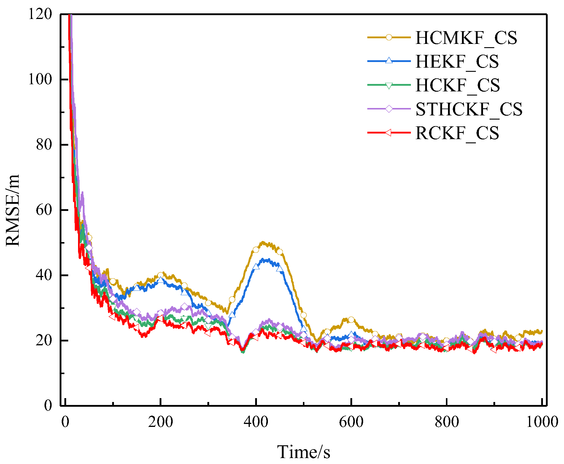
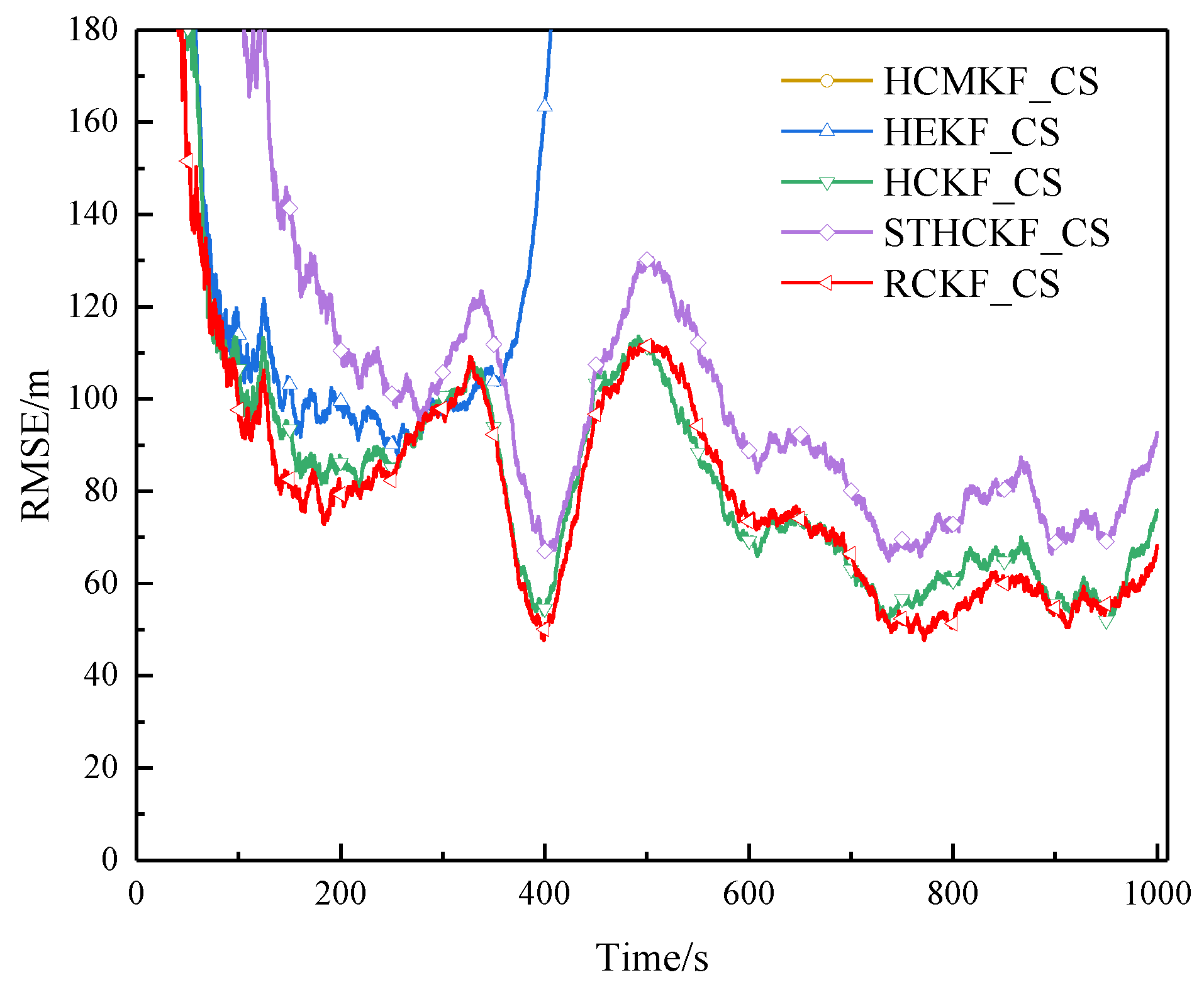
Electronics 14 01973 g011
Figure 12. RMSE of example 1 in surface track 3 (Experiment A).
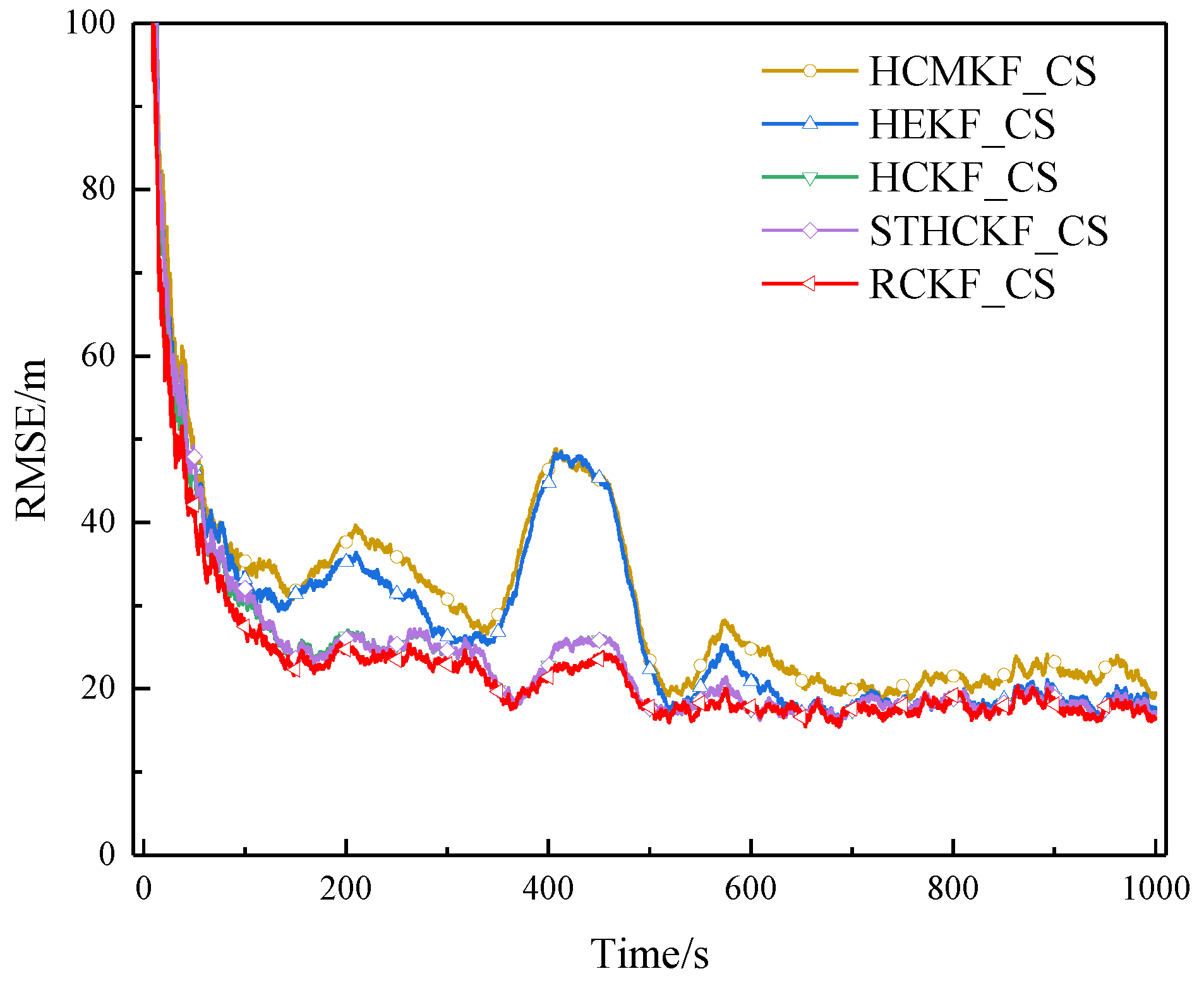
Electronics 14 01973 g012
Figure 13. RMSE of example 2 in surface track 3 (Experiment A).
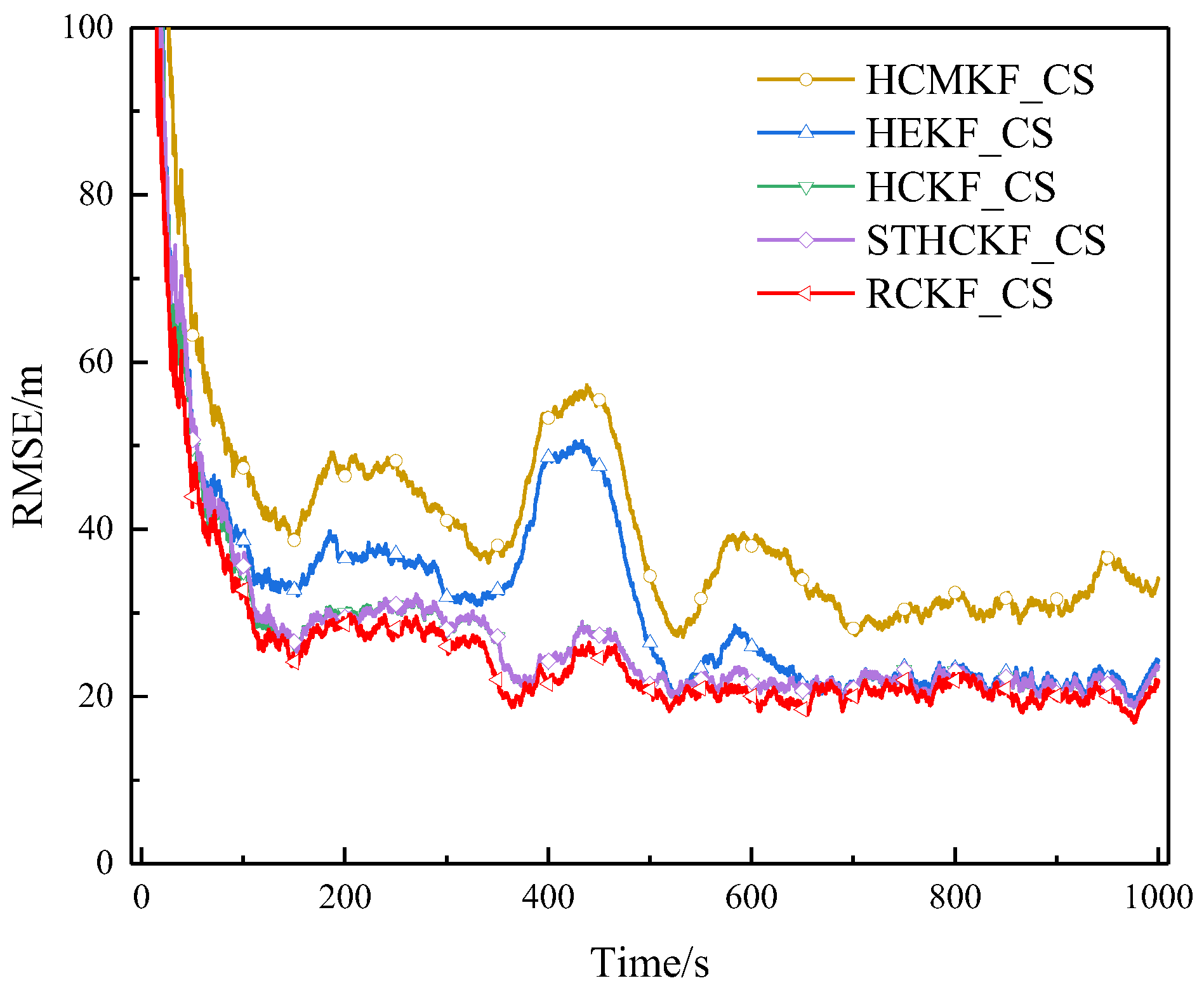
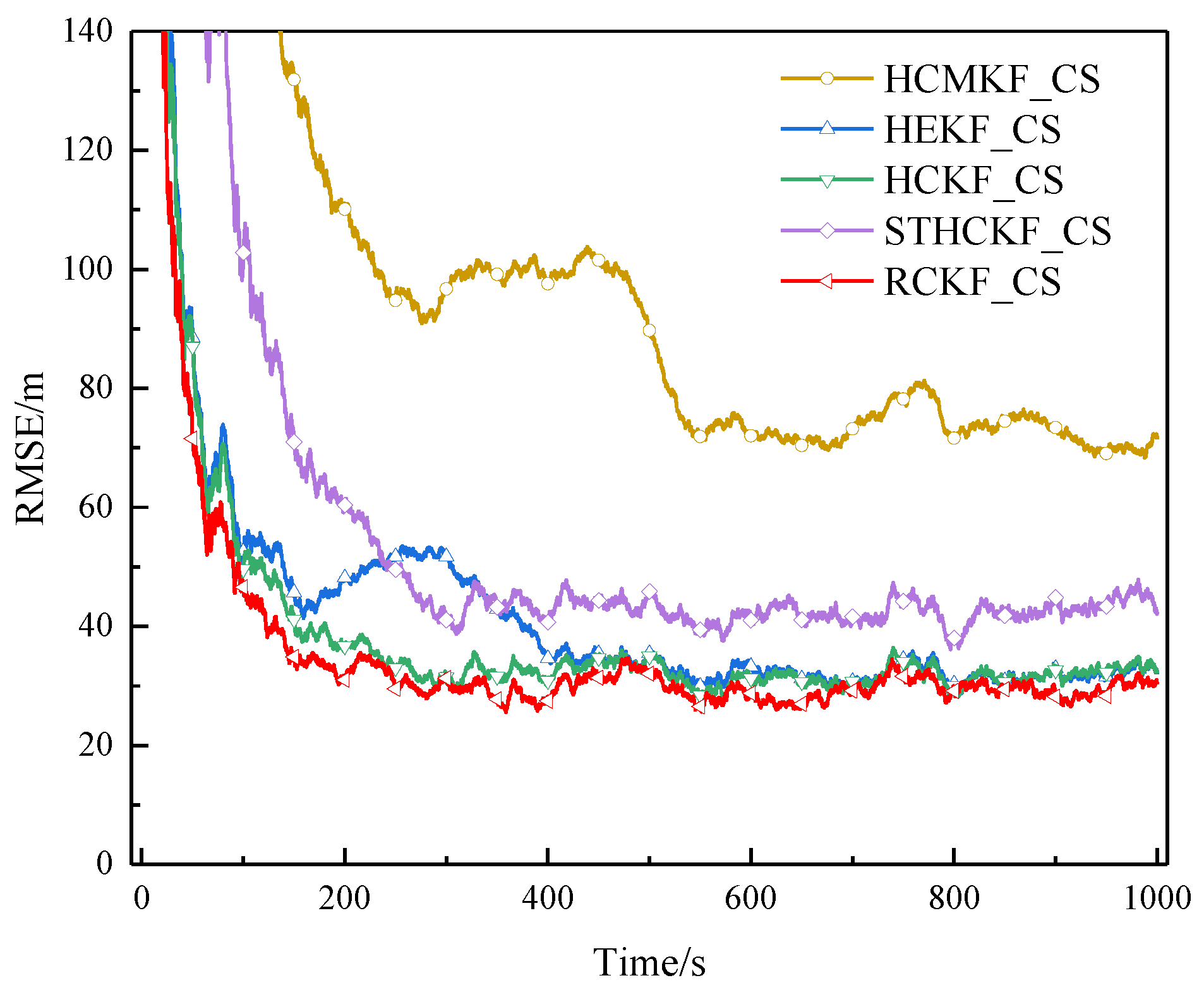
Electronics 14 01973 g013
Figure 14. RMSE of example 3 in surface track 3 (Experiment A).
Electronics 14 01973 g014
Figure 15. RMSE of example 1 in surface track 4 (Experiment A).
Electronics 14 01973 g015
Figure 16. RMSE of example 2 in surface track 4 (Experiment A).
Electronics 14 01973 g016
Figure 17. RMSE of example 3 in surface track 4 (Experiment A).
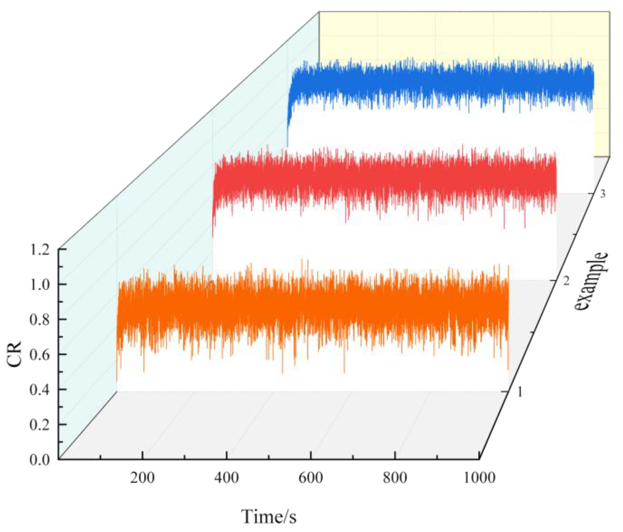
Electronics 14 01973 g017
Figure 18. Condition number ratio curve of surface track 1 (Experiment A).
Electronics 14 01973 g018
Figure 19. Condition number ratio curve of surface track 2 (Experiment A).
Electronics 14 01973 g019
Figure 20. Condition number ratio curve of surface track 3 (Experiment A).
Electronics 14 01973 g020
Figure 21. Condition number ratio curve of surface track 4 (Experiment A).
Electronics 14 01973 g021
Figure 22. RMSE of example 1 in surface track 1 (Experiment B).
Electronics 14 01973 g022
Figure 23. RMSE of example 2 in surface track 1 (Experiment B).
Electronics 14 01973 g023
Figure 24. RMSE of example 3 in surface track 1 (Experiment B).
Electronics 14 01973 g024
Figure 25. RMSE of example 1 in surface track 2 (Experiment B).
Electronics 14 01973 g025
Figure 26. RMSE of example 2 in surface track 2 (Experiment B).
Electronics 14 01973 g026
Figure 27. RMSE of example 3 in surface track 2 (Experiment B).
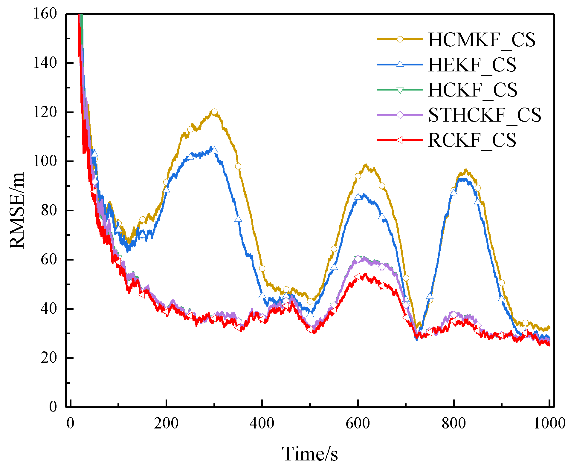
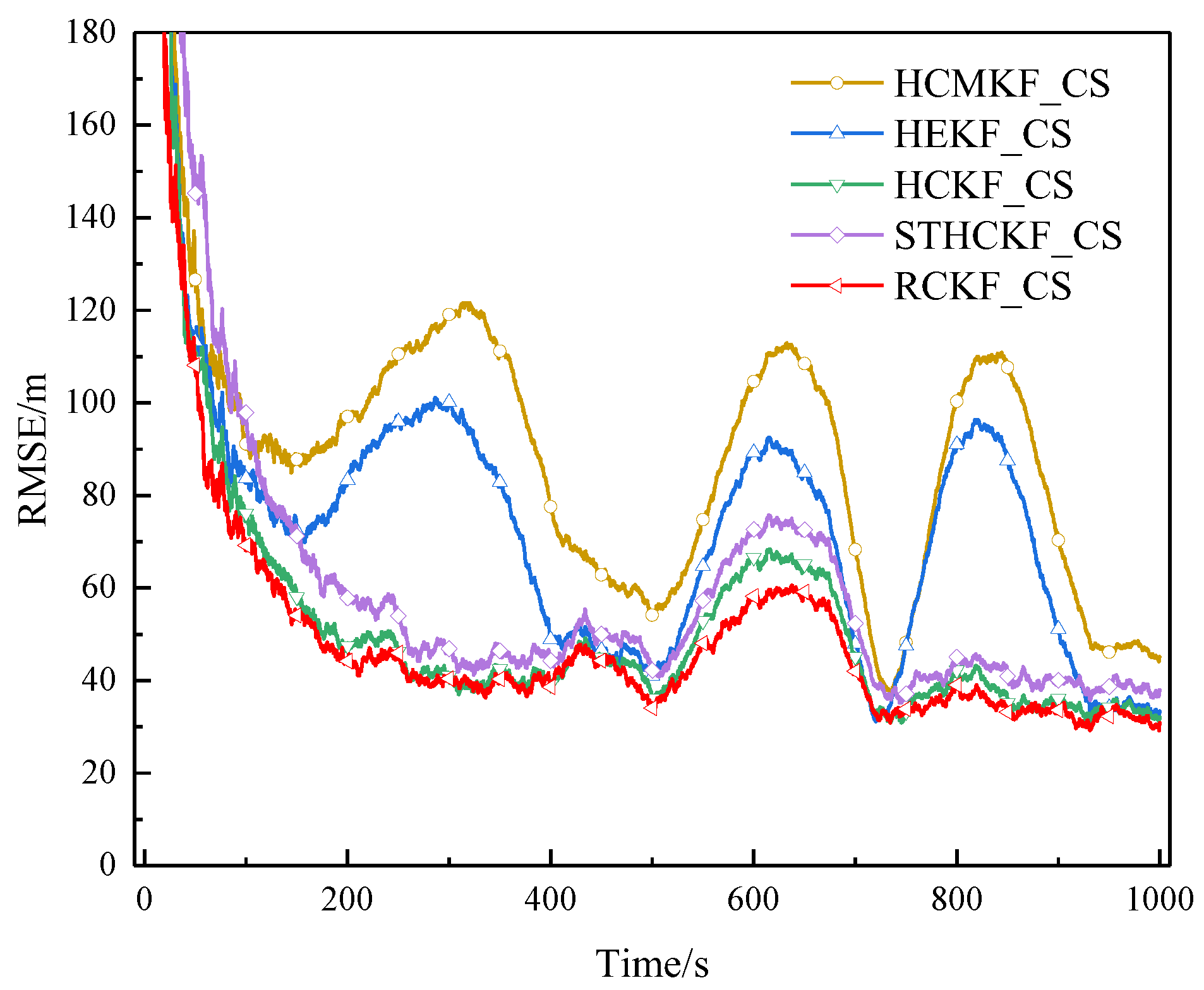
Electronics 14 01973 g027
Figure 28. RMSE of example 1 in surface track 3 (Experiment B).
Electronics 14 01973 g028
Figure 29. RMSE of example 2 in surface track 3 (Experiment B).
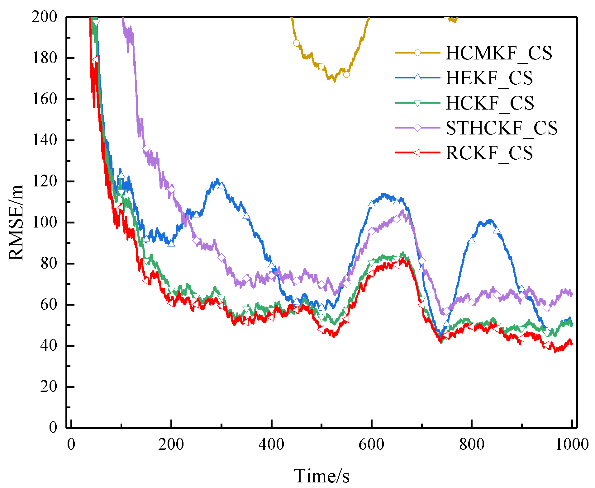
Electronics 14 01973 g029
Figure 30. RMSE of example 3 in surface track 3 (Experiment B).
Electronics 14 01973 g030
Figure 31. RMSE of example 1 in surface track 4 (Experiment B).
Electronics 14 01973 g031
Figure 32. RMSE of example 2 in surface track 4 (Experiment B).
Electronics 14 01973 g032
Figure 33. RMSE of example 3 in surface track 4 (Experiment B).
Electronics 14 01973 g033
Figure 34. Condition number ratio curve of surface track 1 (Experiment B).
Electronics 14 01973 g034
Figure 35. Condition number ratio curve of surface track 2 (Experiment B).
Electronics 14 01973 g035
Figure 36. Condition number ratio curve of surface track 3 (Experiment B).
Electronics 14 01973 g036
Figure 37. Condition number ratio curve of surface track 4 (Experiment B).
Electronics 14 01973 g037
Table 1. Notations and definitions of variables in Section 4.
SymbolDefinitionSymbolDefinition
δ x k / k 1 The error between the extrapolated estimate value of the state and the true value λ k Adaptive factor for residual suppression
v k Measurement noise (also used as residual) γ Threshold in penalty strategy
ε k Composite error vector τ Slope control parameter in exponential penalty
ξ k Normalised error vector η Upper bound in penalty function
S k Covariance matrix R k Measurement noise covariance matrix
J X k The loss function at moment k P k A posteriori state covariance matrix
ρ ( · ) Penalty function (piecewise-defined smooth approximation) x ^ k Estimated state after correction
ϕ k Quadratic term in loss function K k Kalman gain
Table 2. List of simulation conditions.
Simulation ParameterValue
Number of simulations200
Radar sampling time (s)1000
Sampling interval (s)0.1
Standard deviation of radar range noise (m)50
Standard deviation of angle noise (°)0.5
Pollution rate ε of example 1 of each track0.1
Pollution rate ε of example 2 of each track0.2
Pollution rate ε of example 3 of each track0.4
Acceleration maximum value of the CS model (m/s2)0.1
Table 3. Different parameter combinations of the adaptive factor with the penalty strategy.
η
Smoothing Threshold
τ
Penalty Sharpness
γ
Gain Suppression Level
P 1 101004.25
P 2 101005.25
P 3 201004.25
P 4 201005.25
P 5 101504.25
P 6 101505.25
P 7 201504.25
P 8 201505.25
Table 4. Test results of the experiments for the parameter settings (Experiment A) (m).
P 1 P 2 P 3 P 4 P 5 P 6 P 7 P 8
Track 1/ε = 0.118.53919.03118.56518.90818.98919.07618.96318.714
Track 1/ε = 0.221.31821.97821.42921.96121.75022.24121.54822.180
Track 1/ε = 0.429.93731.03529.83231.08730.92132.32730.24132.178
Track 2/ε = 0.119.17919.83119.27419.69319.57519.43819.47719.669
Track 2/ε = 0.221.93822.91521.71223.02822.14522.80821.74622.885
Track 2/ε = 0.430.49232.38630.96532.12931.84832.91931.39633.874
Track 3/ε = 0.149.76351.49349.71050.76250.80251.35149.94552.022
Track 3/ε = 0.256.56857.55056.75256.90656.96157.45056.87957.248
Track 3/ε = 0.475.91376.91974.96578.37476.37278.57676.77878.678
Track 4/ε = 0.135.60236.31436.11936.64736.42136.06736.26136.891
Track 4/ε = 0.241.11941.60740.68342.15741.38743.04841.47342.527
Track 4/ε = 0.456.07759.06256.78559.64056.05960.37357.64960.438
Table 5. Test results of the experiments for the parameter settings (Experiment B) (m).
P 1 P 2 P 3 P 4 P 5 P 6 P 7 P 8
Track 1/ε = 0.118.54818.94018.60718.78418.61618.75418.75019.147
Track 1/ε = 0.221.14924.29521.32422.29621.81022.15321.27223.385
Track 1/ε = 0.429.30732.07929.55331.46130.83532.51730.29932.115
Track 2/ε = 0.119.56819.62019.38819.48819.21519.45519.16319.755
Track 2/ε = 0.222.35622.96422.10322.66122.52123.18422.18023.038
Track 2/ε = 0.430.79332.73331.00632.44831.41533.11631.18633.580
Track 3/ε = 0.150.79551.13350.01250.33450.31651.14251.49950.421
Track 3/ε = 0.256.41357.62357.08856.96657.37157.92457.76257.685
Track 3/ε = 0.474.57577.46674.60178.46275.09978.13174.74778.772
Track 4/ε = 0.136.13436.35536.20436.90337.04837.28936.24936.446
Track 4/ε = 0.241.39641.88940.71942.82241.37242.30242.02242.515
Track 4/ε = 0.456.22858.52956.23358.64457.36259.85758.64359.645
Table 6. Average RMSE of surface track 1 (Experiment A) (m).
ApproachHCMKF_CSHEKF_CSHCKF_CSSTHCKF_CSRCKF_CS δ
ε = 0.123.73821.46218.99519.00418.4902.66%
ε = 0.233.94726.15922.81522.84621.3906.25%
ε = 0.485.03234.45131.41731.48029.6785.54%
(Note: δ = The   Average   RMSE   of   HCKF _ CS The   average   RMSE   of   RCKF _ CS The   Average   RMSE   of   HCKF _ CS × 100 % ).
Table 7. Average RMSE of surface track 2 (Experiment A) (m).
ApproachHCMKF_CSHEKF_CSHCKF_CSSTHCKF_CSRCKF_CS δ
ε = 0.127.37024.85320.25220.25719.3504.45%
ε = 0.237.36328.40323.66023.66821.9967.03%
ε = 0.487.74839.60632.72932.76630.4377.00%
(Note: δ = The   Average   RMSE   of   HCKF _ CS The   average   RMSE   of   RCKF _ CS The   Average   RMSE   of   HCKF _ CS × 100 % ).
Table 8. Average RMSE of surface track 3 (Experiment A) (m).
ApproachHCMKF_CSHEKF_CSHCKF_CSSTHCKF_CSRCKF_CS δ
ε = 0.1411.688343.49955.49055.20149.84010.18%
ε = 0.2591.392491.39161.52061.04756.9267.47%
ε = 0.4572.914622.33479.58078.98275.8564.68%
(Note: δ = The   Average   RMSE   of   HCKF _ CS The   average   RMSE   of   RCKF _ CS The   Average   RMSE   of   HCKF _ CS × 100 % ).
Table 9. Average RMSE of surface track 4 (Experiment A) (m).
ApproachHCMKF_CSHEKF_CSHCKF_CSSTHCKF_CSRCKF_CS δ
ε = 0.171.90664.13038.69838.66336.6175.38%
ε = 0.280.58964.90942.52442.45340.2815.27%
ε = 0.4313.26982.75159.99259.88156.4895.84%
(Note: δ = The   Average   RMSE   of   HCKF _ CS The   average   RMSE   of   RCKF _ CS The   Average   RMSE   of   HCKF _ CS × 100 % ).
Table 10. Average RMSE of surface track 1 (Experiment B) (m).
ApproachHCMKF_CSHEKF_CSHCKF_CSSTHCKF_CSRCKF_CS δ
ε = 0.123.84022.04719.13020.25818.2304.70%
ε = 0.233.18625.44322.25825.52821.1964.77%
ε = 0.483.21536.15732.25543.65429.7898.61%
(Note: δ = The   Average   RMSE   of   HCKF _ CS The   average   RMSE   of   RCKF _ CS The   Average   RMSE   of   HCKF _ CS × 100 % ).
Table 11. Average RMSE of surface track 2 (Experiment B) (m).
ApproachHCMKF_CSHEKF_CSHCKF_CSSTHCKF_CSRCKF_CS δ
ε = 0.128.10725.03620.51121.98619.7433.74%
ε = 0.237.97428.37024.10827.70222.4966.69%
ε = 0.489.22939.32233.02544.65930.8566.57%
(Note: δ = The   Average   RMSE   of   HCKF _ CS The   average   RMSE   of   RCKF _ CS The   Average   RMSE   of   HCKF _ CS × 100 % ).
Table 12. Average RMSE of surface track 3 (Experiment B) (m).
ApproachHCMKF_CSHEKF_CSHCKF_CSSTHCKF_CSRCKF_CS δ
ε = 0.1462.053533.85055.93559.19150.6689.42%
ε = 0.2529.017350.95960.74767.51056.2877.34%
ε = 0.4476.740653.20776.06791.23573.3653.55%
(Note: δ = The   Average   RMSE   of   HCKF _ CS The   average   RMSE   of   RCKF _ CS The   Average   RMSE   of   HCKF _ CS × 100 % ).
Table 13. Average RMSE of surface track 4 (Experiment B) (m).
ApproachHCMKF_CSHEKF_CSHCKF_CSSTHCKF_CSRCKF_CS δ
ε = 0.166.28361.60238.40340.85535.7576.89%
ε = 0.283.58267.17843.74449.05640.9896.30%
ε = 0.4249.53082.80058.80076.07155.0706.34%
(Note: δ = The   Average   RMSE   of   HCKF _ CS The   average   RMSE   of   RCKF _ CS The   Average   RMSE   of   HCKF _ CS × 100 % ).
Disclaimer/Publisher’s Note: The statements, opinions and data contained in all publications are solely those of the individual author(s) and contributor(s) and not of MDPI and/or the editor(s). MDPI and/or the editor(s) disclaim responsibility for any injury to people or property resulting from any ideas, methods, instructions or products referred to in the content.

