A Sea-Surface Radar Target-Detection Method Based on an Improved U-Net and Its FPGA Implementation

Abstract

Existing radar target-detection methods exhibit suboptimal performance when they are applied to sea-surface target detection. This is due to the difficulties in detecting weak targets and the interference from sea clutter, as well as to the inability of statistical models to accurately model sea-surface targets, which leads to degraded detection performance. With the development of artificial intelligence technologies, research based on deep learning methods has gained momentum in the field of radar target detection. Considering the complexity of neural networks and the real-time requirements of radar target-detection algorithms, this paper investigates a sea-surface radar target-detection method based on an improved U-Net network and its FPGA implementation, achieving real-time radar target detection without relying on GPUs. This paper first selected the lightweight U-Net network through a survey and analysis. The original U-Net network was then structurally optimized using network volume-reduction methods. Based on the characteristics of the network structure, optimization strategies such as pipelining and parallel processing, hybrid-layer design, and convolution-layer optimization were applied to the accelerator system. These optimizations reduced the system’s hardware-resource requirements and enabled the complete deployment of the network onto the accelerator system. The accelerator system was implemented using high-level synthesis (HLS) with modular and template-based design approaches. Experiments showed that the proposed method has significant advantages in improving detection probability, reducing false-alarm rates, and achieving real-time processing.

1. Introduction

Radar sea-surface target detection is a crucial aspect of maritime surveillance, with significant applications in monitoring of maritime traffic and navigation safety. Traditional radar target-detection methods primarily rely on statistical and non-linear techniques in the time, frequency, and transform domains to achieve robust target detection. However, these methods often suffer from model-mismatch issues. To address the potential mismatch of statistical models, research based on machine learning methods has gained momentum in the field of sea-surface small-target detection.

Since 2012, the development roadmap of convolutional neural network (CNN) object-detection algorithms has seen a series of innovations and breakthroughs. CNN models evolved from AlexNet [1] to VGGNet [2], then to GoogleNet [3] and ResNet [4], among others. In the field of image-object detection based on CNN, algorithms have progressed from region proposal-based methods such as RCNN [5], which evolved into Fast R-CNN [6] and Faster R-CNN [7], to regression-based methods including You Only Look Once (YOLO) [8,9,10,11] and Single Shot Detector (SSD) [12]. These advancements have led to significant improvements in both detection speed and accuracy.

In the field of radar target detection, an increasing number of researchers have attempted to apply deep learning algorithms to solve radar target-detection problems and have published a series of research results with high theoretical significance and practical value. The rapid development of deep learning in recent years has led to significant progress in the field of object detection, opening up new possibilities for research in radar target detection, especially for sea-surface target detection.

Work by Loran et al. (2023) [13] involved the implementation of a radar target detector based on the Faster R-CNN model. The proposed ship detector was tested for robustness in various scenarios and demonstrated high recall rates even in very dense multi-target scenes. Huang et al. (2023) [14] addressed the challenge of weak signal detection in non-cooperative bistatic radar by proposing to enhance detection performance through the improved YOLOv5s network. The improvements included adding skip connections and introducing attention mechanisms, which significantly improved the accuracy of detection of weak targets. Wang et al. (2024) [15] proposed a deep learning-based method for target detection in environments with sea clutter, extracting multiple features from range profiles and range-Doppler spectra for sea-surface target detection. Experiments proved that this method outperformed the classical constant false alarm rate algorithm in detection capability.

Despite the good detection capabilities of deep learning-based methods for radar targets, considering the real-time requirements of radar target-detection algorithms, CNNs require substantial processing power and memory bandwidth and currently rely on GPUs with high energy consumption to meet real-time processing demands. With the advantages of high performance, strong reconfigurability, and short development cycles, FPGAs have begun to be applied in various CNN accelerators.

Liang et al. (2014) [16] proposed converting deep learning algorithms into hardware description language (HDL) using the HLS tools, combining these with loop unrolling and pipelining optimization techniques to reduce the computational complexity and storage requirements of the models. This method implemented CNNs on FPGAs, improving computational speed under low-power conditions. Nguyen et al. (2024) [17] proposed an FPGA-based YOLOv4 network design with optimizations for model parameter selection, model quantization, and network architecture. Experiments showed that this method could run in real time on FPGAs while maintaining accuracy. Zeng et al. (2020) [18] designed a heterogeneous “CPU+FPGA” system to accelerate the computation of Graph Convolutional Networks (GCN), using systolic arrays for efficient parallelization and full pipelining to achieve load balancing and improve DSP utilization.

It can be seen that FPGA is suitable for accelerating CNN computational tasks. The programmability and reconfigurability of FPGA allow accelerator designs to be evaluated in a short period of time. In particular, the emergence of the HLS tools has significantly shortened the development cycle and saved on design and development costs. However, regarding the deployment of radar applications for deep learning-based detection models, there are currently few related studies on the implementation of radar-based detection algorithms based on CNN on FPGA. There are still problems, such as the mismatch between the computing throughput and the FPGA memory bandwidth, and the space for accelerator design is not fully utilized. Reference [19] transferred the deep neural network target-detection and -recognition model used in the visible-light data domain to the radar-echo data domain and conducted lightweight tests, but no related work on embedded development and deployment was carried out. Reference [20] integrated the traditional Constant False Alarm Rate (CFAR) algorithm with the Faster R-CNN model to form a lightweight radar target-detection algorithm, and no lightweight deployment work has been carried out.

This paper aims to address the limitations of traditional radar detection algorithms in complex sea conditions and the challenges of deploying deep learning-based detection models on radar systems. This paper selected the high-performance lightweight CNN to construct the radar target-detection algorithm and optimized it for deployment on general FPGA devices. This paper is organized into five parts:

• Implementation of a machine learning-based detection process: research on target-detection algorithms based on CNNs, analysis of the advantages of target-detection algorithms based on CNNs, and selection of high-performance lightweight networks as detection networks.
• Network optimization: in response to the lightweight requirements of FPGA deployment, methods such as depthwise separable convolutions (DSC), inverted residual structures, and atrous spatial pyramid pooling (ASPP) are used to structurally optimize the original networks.
• Acceleration architecture: a flexible RDMA-based acceleration architecture maps each layer of the network to an independent hardware pipeline stage on the FPGA. Each network layer’s acceleration hardware can be individually optimized based on its characteristics, achieving high hardware utilization and improved throughput.
• Optimization of FPGA implementation: to align with the network structure, the accelerator system is optimized using strategies such as pipelining, parallel processing, fine-grained quantization, and hybrid layer design.
• FPGA implementation results: on the Xilinx KCU1500 FPGA development board, a real-time target-detection system is achieved based on the HW-UNet, and its effectiveness is validated using the collected data. Compared with traditional target-detection algorithms such as Cell-Averaging Constant False Alarm Rate( CA-CFAR) detection, the superiority of the CNN-based approach is demonstrated.

2. Radar Sea-Surface Target-Detection Method Based on Neural Networks

2.1. Machine Learning Detection Workflow

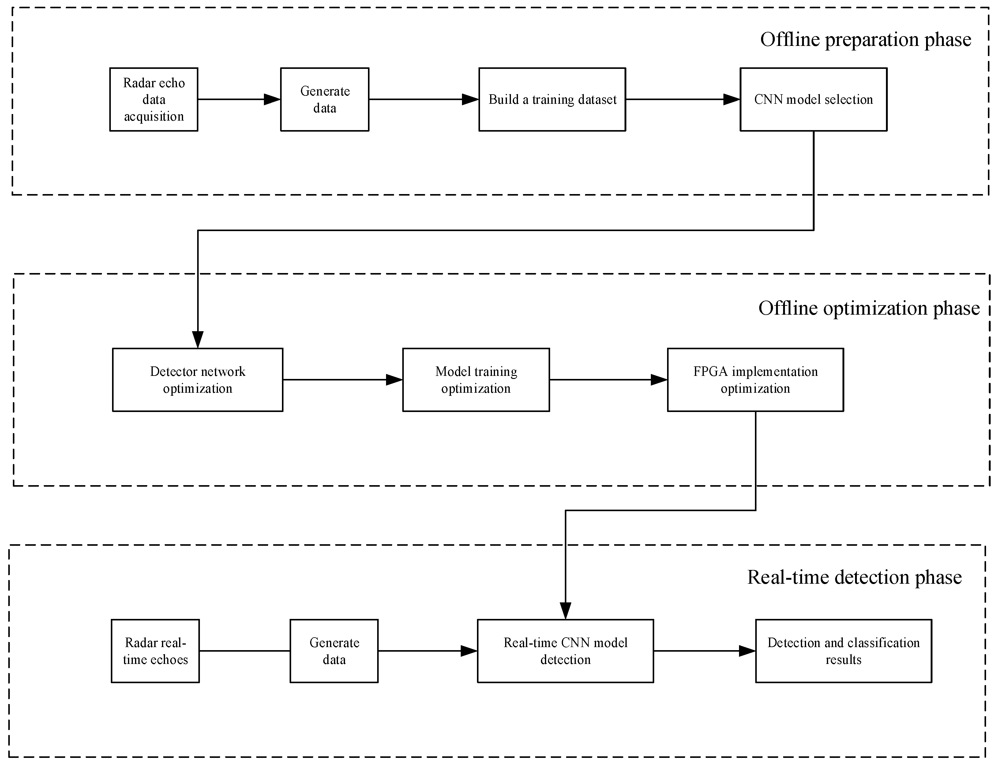
Deep learning is a type of deep neural network that utilizes multiple hidden layers to learn the features of input data. It distinguishes targets from backgrounds by classification, thereby achieving target detection. The working principle of a deep learning-based radar detector is shown in Figure 1.

The working process of a deep learning-based detector mainly consists of three stages: offline preparation, offline optimization, and real-time detection. In the offline preparation stage, the echo data of different types of radar sea-surface targets (dense multiple targets; large, medium, and small targets; and maneuvering targets) are collected and stored under various conditions (different sea states, weather conditions, sampling frequencies, pulse lengths, etc.). Subsequently, after cropping and labeling, a comprehensive sea-surface target dataset is constructed and a suitable neural network is selected.

In the offline optimization stage, the neural network is optimized for lightweight deployment, reducing parameters and computational load. The detector is trained using samples composed of radar sea-surface target echo data and corresponding labels. The labels are set to values of 1 or 0 based on whether the echo data contain sea-surface targets. The dataset is input into the optimized CNN model for training and iterative optimization to obtain the optimal target-detection model. Subsequently, to enhance the efficiency of FPGA implementation, the process of deploying neural networks on the FPGA is optimized to achieve the optimal program for running the target-detection model on the FPGA.

In the real-time detection stage, the trained target-detection model is used to detect sea-surface targets. Real-time radar echo data are input into the model, and the final detection results are obtained directly.

Compared with classical sea-surface target-detection methods, CNN-based methods exhibit stronger detection capabilities due to their ability to learn target features deeply during training.

2.2. Neural Network Selection

In the field of computer vision, object detection and semantic segmentation are two key tasks. Specifically, object detection aims to identify objects in images or videos and provide their locations, while semantic segmentation assigns each pixel in an image to a specific category, achieving fine-grained image segmentation.

Deep learning-based object-detection methods are a type of feature-detection approach. Neural networks are primarily divided into two-stage detection methods and one-stage detection methods. Region-based object-detection algorithms first determine candidate regions using selective search methods and then employ deep learning techniques to extract features and classify objects within these regions. Since the detection process involves two steps, this approach is also known as a two-stage detection algorithm. Common algorithms include Fast R-CNN and Faster R-CNN. Although region-based object detection algorithms achieve high detection performance, their speed is insufficient for real-time detection requirements. To address this issue, researchers have proposed regression-based object-detection algorithms. These algorithms adopt an end-to-end detection approach, performing only a single forward pass through the network, which significantly improves detection speed. Regression-based object-detection algorithms treat object detection as a regression problem, eliminating the separate region-proposal stage and directly regressing the classification probabilities and location coordinates of objects. This one-step detection process is also called a one-stage detection algorithm. Common algorithms in this category include YOLO and SSD.

For radar target detection, downsampling operations can lead to significant feature loss, especially for radar echo targets that occupy few data units in the input data. This loss is exacerbated by the use of multiple downsampling layers, which results in weak semantic information in the output feature maps and makes accurate detection challenging. In applications such as robotics, automotive systems, medical imaging, and other embedded systems that require scene understanding, semantic image segmentation is crucial for intelligent functionality. Many recent studies on deep learning have focused on semantic segmentation tasks. The U-Net, proposed by Olaf Ronneberger et al., is a U-shaped network architecture [21] that improves upon the Fully Convolutional Networks (FCN) design philosophy, achieving pixel-level semantic segmentation. U-Net’s encoder–decoder architecture combines low-level encoder features with upsampled decoder features using skip connections, which helps recover spatial details lost during downsampling and improves segmentation accuracy. Importantly, U-Net is built upon the principles of CNNs, which lay a solid foundation for its effective use in segmentation. In radar target detection, the detection environment typically involves complex sea-clutter backgrounds, which may contain various textures and structures. Weak targets closely resemble the background, making it challenging to distinguish them from the background. The U-shaped network’s powerful feature-extraction capabilities, combined with pixel-level feature-extraction methods, can effectively extract the texture and edge features of small sea-surface targets, thereby enhancing detection accuracy.

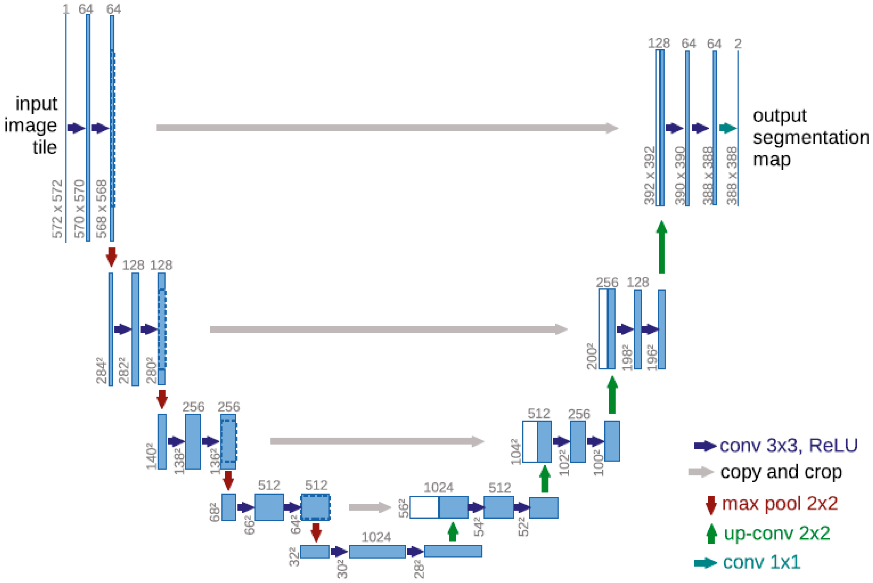
2.3. Classical U-Net Network

The classical U-Net FCN typically consists of five components: convolutional layers, transposed convolutional layers, pooling layers, upsampling layers, and activation function layers. The downsampling network is constructed by stacking two convolutional layers for feature extraction and one max-pooling layer for downsampling. The upsampling network is constructed using transposed convolutional layers. As a derivative of fully convolutional networks, U-Net introduces skip connections to fuse information across layers, connecting the downsampling and upsampling layers. This architecture allows the output data to maintain the same spatial dimensions as the input data.

Thanks to its powerful feature-extraction capabilities, U-Net requires only a small amount of data for training. However, the original network model has a large number of parameters and computational requirements, making it necessary to optimize the network for lightweight deployment on FPGA devices.

3. Detector Network-Optimization Methods

Since the network model must be deployed on FPGAs, there are stringent constraints on both the computational complexity and the number of parameters in the network model. Therefore, the network must be optimized through lightweight design to reduce the computational and storage resources required by the network model. However, the question of how to reduce the computational load and number of parameters in the network model while ensuring accuracy is a challenge in the design of lightweight networks. In order to balance accuracy and model size while utilizing the redundancy and fault tolerance of deep learning models to achieve efficient compression of deep model parameters, this paper mainly focuses on lightweight structural optimization of the model through network structure design. Taking DSC modules, inverted residual structure modules, and ASPP modules as models, this work designs a new CNN based on the U-Net architecture that is highly accurate and has few parameters and low computational complexity. This network was named HW-UNet.

3.1. Depthwise Separable Convolution

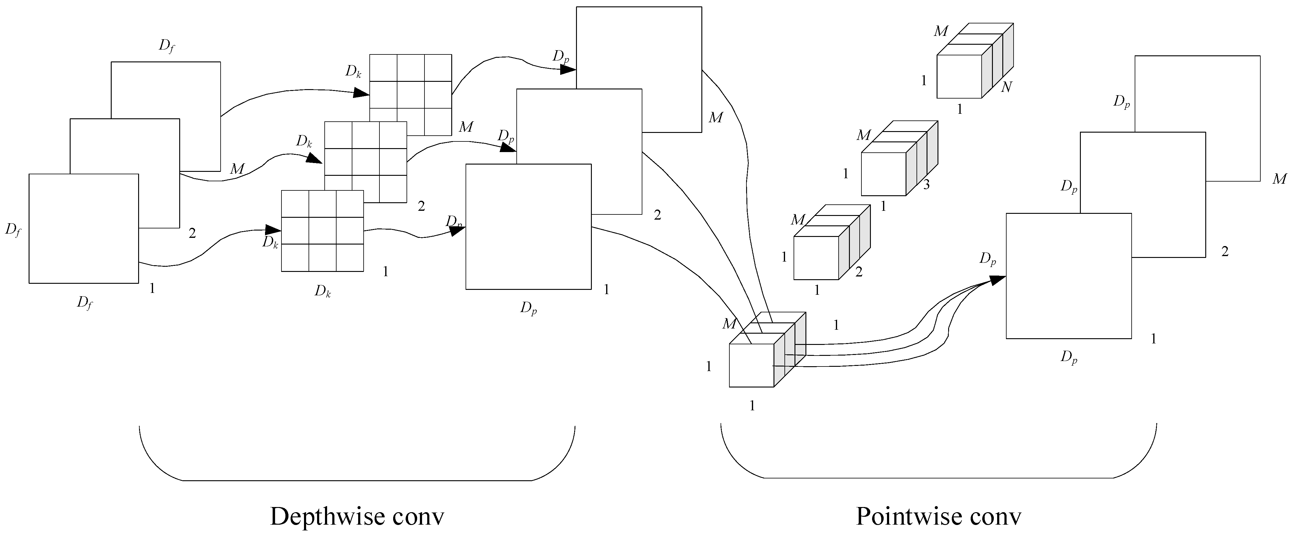
Howard et al. proposed a lightweight and efficient CNN model called MobileNet [22] (Efficient Convolutional Neural Networks for Mobile Vision Applications), which employs DSC. In this approach, depthwise convolution (DWC) performs spatial convolution operations independently on each input channel, while pointwise convolution (PWC) combines the resulting feature maps, as illustrated in Figure 2. DSC consists of DWC and PWC. Compared to standard convolution, DSC decomposes the convolution operation into two steps. DWC is responsible for feature extraction, while PWC is used to fuse information and expand the dimensionality of the feature maps.

Unlike standard convolution, the number of convolution kernels in DWC is determined by the number of input channels, with each kernel operating on a single channel. Therefore, during the DWC operation, each channel of the input feature map is convolved with its corresponding kernel. The outputs from all kernels are then concatenated along the channel axis to form the output feature map, as shown in Figure 2.

Since DWC maintains the same number of input and output channels without expanding the feature map, it can be regarded as an extreme form of group convolution (GC), where each channel is convolved separately. This approach does not effectively utilize the information across channels. Therefore, PWC is necessary to extract and fuse feature information from all channels at each spatial location. Each convolution kernel in PWC has the same number of channels as the input feature map, and the number of kernels corresponds to the number of output channels. The convolution process is also depicted in Figure 2.

Let the input feature map F have dimensions D_f × D_f × M and the output feature map G have dimensions D_p × D_p × N. Here, D_f represents the width and height of the input feature map, M denotes the number of input channels, and N denotes the number of output channels. The kernel size for standard convolution and DWC was D_K × D_K, while the kernel size for PWC was 1 × 1. The standard convolution process with a stride of 1 and padding is described in Equation (1), as follows:

$$G_{k,l,n}={\displaystyle \sum _{i,j,m}{K}_{i,j,m,n}\times F_{k+i-1,l+j-1,m}}$$

(1)

In Equation (1), K represents the filter of the standard convolution, with the input image denoted as F and the output image denoted as G. For standard convolution, the computational cost is given by Equation (2), as follows:

$$O{A}_{SC}=D_f^2\times M\times N\times D_K^2$$

(2)

The DWC operation of the filter is described in Equation (3), as follows:

$$G_{k,l,m}^{\prime }={\displaystyle \sum _{i,j}{K}_{i,j,m}^{\prime }\times F_{k+i-1,l+j-1,m}}$$

(3)

In Equation (3), the filter for DWC is denoted as $K^{\prime }$ and the output feature map is represented as $G^{\prime }$. Here, m indicates that the m-th filter was applied to the m-th feature map of F, generating the m-th feature map in $G^{\prime }$. The computational cost of DWC is shown in Equation (4), while the computational cost of PWC is given by Equation (5), as follows:

$$O{A}_{DWC}=D_f^2\times M\times D_K^2$$

(4)

$$O{A}_{PWC}=D_f^2\times 1\times 1\times M\times N$$

(5)

The ratio of the computational costs between traditional standard convolution and DSC is shown in Equation (6), as follows:

$${\displaystyle \frac{D_f^2\times M\times D_K^2+D_f^2\times 1\times 1\times M\times N}{D_f^2\times M\times N\times D_K^2}}={\displaystyle \frac{1}{N}}+{\displaystyle \frac{1}{D_K^2}}$$

(6)

Furthermore, a comparison of the parameter counts for the two convolution structures was conducted. The parameter count for standard convolution is given by Equation (7), while the parameter count for DSC is shown in Equation (8), as follows:

$$P{A}_{SC}=M\times N\times D_f^2$$

(7)

$$P{A}_{DSC}=M\times (D_K^2\times N)$$

(8)

From the above analysis, it is evident that DSC offers the advantage of significantly reducing the number of model parameters and the computational load while maintaining or even improving performance compared to standard convolution. Therefore, in this paper, we optimized the network architecture by replacing the standard convolution in the encoder with DSC modules. Additionally, since consecutive max-pooling operations in the encoder path can reduce image resolution, we replaced the max-pooling operations in the first to fourth layers of the encoder in the backbone network with DSC with a stride of 2 to enhance the segmentation performance of the network. This optimization not only reduced the computational complexity but also maintained the spatial resolution of the feature maps, which is crucial for accurate target detection.

3.2. Inverted Residual Structure

Traditional residual structures and inverted residual structures exhibit significant differences in channel-number variations and convolutional-layer designs. The inverted residual structure enhances model efficiency and accuracy by increasing the number of channels in the intermediate layers and employing DSC while maintaining low computational cost and memory usage. This design is particularly suitable for low-power devices and embedded systems.

In traditional residual structures, the input and output channels are numerous, while the intermediate convolutional layer has fewer channels, forming a bottleneck structure. In contrast, MobileNetV2 [23] features fewer input and output channels but more channels in the intermediate DSC layer, creating an inverted-bottleneck structure. This design allows the model to maintain low computational cost while effectively extracting features.

In traditional CNNs, convolutional layers typically reduce the number of channels to lower computational cost and then restore the channel count in the decoding stage. However, MobileNetV2 adopts an opposite approach by initially increasing the number of channels, then conducting feature extraction using DSCs and dimensionality reduction using 1 × 1 convolutions. This design effectively utilizes the high-dimensional representation in the intermediate layers and maintains information flow through skip connections.

While DSCs reduce the number of parameters in the network, they can also lead to an increase in the number of layers. Although increased network depth enhances model performance, it can also cause model degradation. Residual structures address this issue by employing a directed curve to simply perform identity mappings, and then element-wise fuse the output of identity mappings with that of the stacked layers. This approach alleviates gradient vanishing and captures rich semantic features, making it widely applicable in tasks such as semantic segmentation.

As previously mentioned, deep residual networks have demonstrated excellent performance in computer vision tasks, especially in semantic segmentation. Therefore, this paper employs a deep residual structure as the backbone network to form a more efficient feature extractor for radar data.

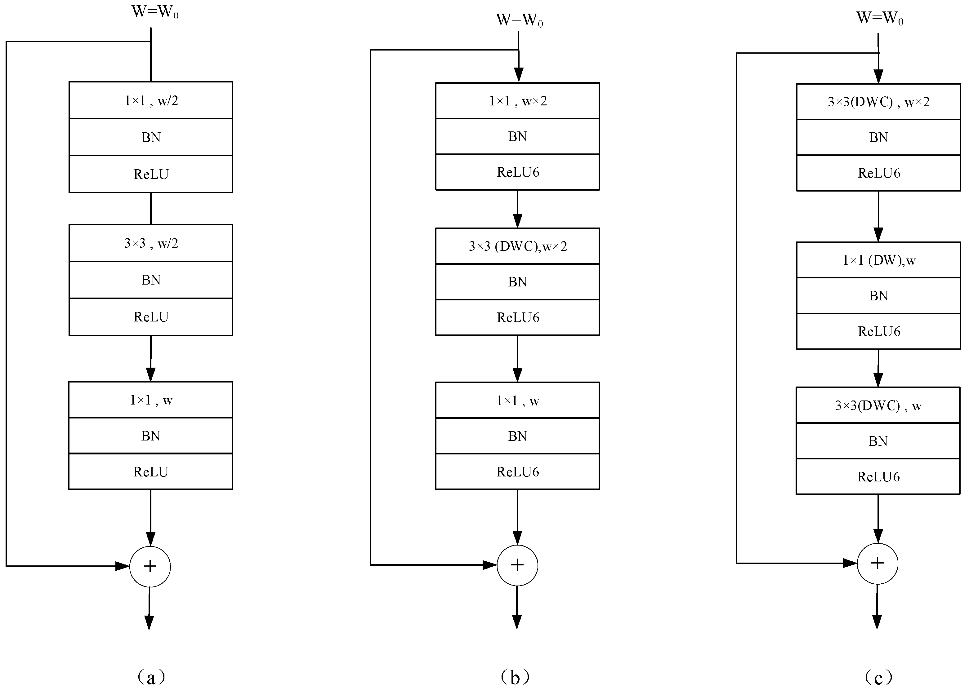
If the input and output feature dimensions are consistent, the feature maps can be directly combined. Otherwise, the input feature map must first be transformed through a 1 × 1 convolutional layer before being concatenated with the input feature map to produce the target feature map. The main difference between the inverted residual structure and the traditional residual structure is as follows. The traditional residual structure first reduces the dimensions of the input feature map using a 1 × 1 convolution, then conducts feature extraction using a 3 × 3 standard convolution, and finally increases the dimensions using another 1 × 1 convolution. The result is then added to the input feature map through channel-wise addition, as shown in Figure 3a. In contrast, the inverted residual structure first increases the dimension using a 1 × 1 convolution, then conducts feature extraction using a 3 × 3 DWC, and finally reduces the dimensionality using another 1 × 1 convolution. The result is then added to the input feature map through channel-wise addition, as shown in Figure 3b.

The reason for using the inverted residual structure is that in DSCs, if the input feature map has a low dimension, a significant portion of the parameters in the DWC kernel are likely to become zero during network training. This means that effective feature extraction is not performed. Therefore, it is necessary to first increase the number of channels in the input feature map before extracting features using DWC. Finally, to reduce the number of parameters and computational load in subsequent convolution kernels, the feature map is reduced in dimension using PWC. However, the PWC convolutional layer used for dimension expansion in the inverted residual structure accounts for most of the computational cost and parameters, making its use not in keeping with the lightweight-design philosophy. Therefore, optimization is necessary.

As shown in Figure 3c, the 1 × 1 convolution expansion component of the inverted residual structure is replaced by a 3 × 3 DWC operation on the input feature map. The resulting feature map is then concatenated with the input feature map, and the concatenated result is used as the output. This Improved Inverted Residual (IIR) structure reduces the computational cost from 1 × 1 × w (assuming the input feature map has w channels, where w is typically 32 or more) to 3 × 3 while retaining the dimension-expansion functionality.

In the inverted residual structure, the ReLU6 activation function is employed. ReLU6 is a clipped version of the Rectified Linear Unit (ReLU) activation function that restricts the output of ReLU to the range of 0 to 6, as shown in Equation (9). In the inverted residual structure, the ReLU6 activation function is typically applied after the expansion layer and after the DSC layer. In the expansion layer, ReLU6 aids in the extraction of non-linear features, while in the DSC layer, ReLU6 helps to extract richer spatial features while maintaining computational efficiency. The activation function following the standard convolution is also ReLU6, which is used with the purpose of limiting all activation values to the range of 0 to 6 to facilitate subsequent hardware deployment.

$$relu6(x)=\left\{\begin{array}{ll}0.0& (x<0)\\ 6.0& (x>6)\\ x& (0\le x\le 6)\end{array}\right.$$

(9)

3.3. Asymmetric Atrous Spatial Pyramid Pooling (AASPP)

ASPP [24] is a deep learning module designed for image-segmentation tasks; it is used with the aim of capturing features at multiple scales to better handle various sizes and shapes of objects in images. The ASPP module has been widely applied in numerous deep learning image-segmentation tasks, such as DeepLabV3 [25] and DeepLabV3+ [26] in the DeepLab series, and has also demonstrated good performance in object-detection tasks.

The AASPP module introduces asymmetric convolutions based on ASPP and reduces some convolution operations and the dilation rates of atrous convolutions, thereby decreasing the number of parameters and computational load. Asymmetric convolutions use a series of asymmetric convolution kernels to replace standard convolution kernels, reducing the convolutional computational load while maintaining the same receptive field. Theoretically, an n × n standard convolution can be replaced by an n × 1 convolution and a 1 × n convolution. The multiplicative computational cost of standard convolution is n × n, while that of asymmetric convolution is 2 × n. As n increases, the reduction in computational operations becomes more significant.

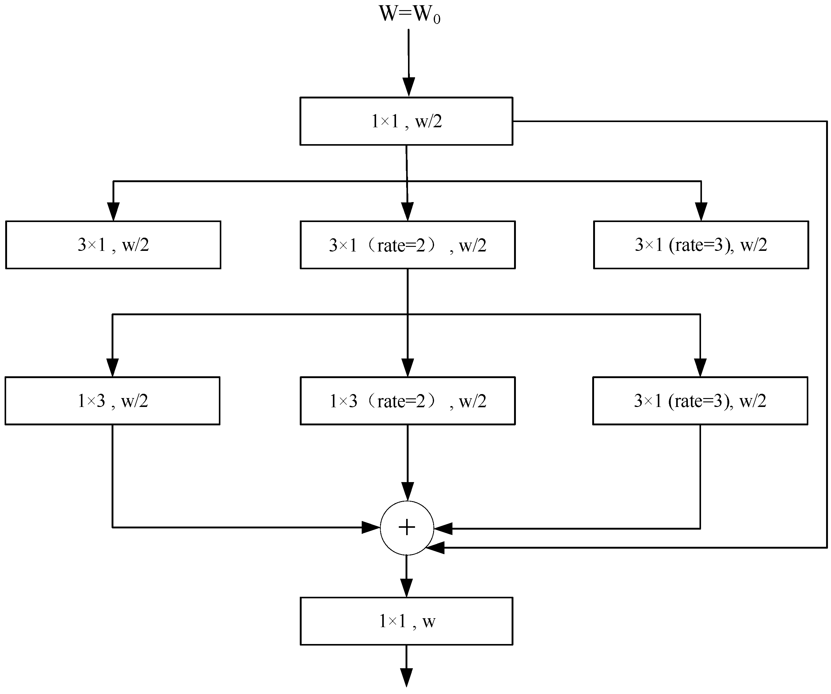
In ASPP, the atrous convolutions used are not depthwise, meaning that each convolution kernel has multiple channels. This increases the number of parameters and computational load. Additionally, the higher dilation rates in ASPP result in a larger sampling range, which requires more storage for hardware deployment. Therefore, optimizations are needed to address these issues. In AASPP, depthwise atrous convolutions are used to replace the original atrous convolutions and the dilation rates of each atrous convolution are reduced. Furthermore, to further decrease the convolutional computational load, asymmetric convolutions are applied to depthwise atrous convolutions, resulting in a convolution method called Depthwise Asymmetric Dilated Convolution (DADC). Finally, a residual connection is added to enhance the representational capability of the module.

The structure of the AASPP module is shown in Figure 4. The module primarily uses dilated convolutions with different dilation rates to obtain feature maps of varying receptive-field sizes, thereby capturing multi-scale information of the segmentation targets. The input feature map first undergoes a PWC to reduce the number of channels to half of the original number. It is then processed in parallel by three sets of convolution kernels, as follows:

• The first set consists of depthwise asymmetric convolutions with kernel sizes of 3 × 1 and 1 × 3.
• The second set consists of depthwise asymmetric dilated convolutions with kernel sizes of 3 × 1 and 1 × 3 with a dilation rate of 2.
• The third set consists of depthwise asymmetric dilated convolutions with kernel sizes of 3 × 1 and 1 × 3 with a dilation rate of 3.

Although dilated convolutions expand the receptive field, they do not introduce additional parameters or increase computational load. The results from these three sets of convolutions are then concatenated with the output of the PWC, doubling the number of channels in the feature map compared to the input. Finally, the concatenated result undergoes another convolution operation, with the output feature map having the same number of channels as the input feature map. This process results in the acquisition of feature maps at different scales and integrates information across channels, effectively increasing the receptive field and merging more contextual features.

3.4. Network Architecture Design

The overall architecture of HW-UNet is similar to that of U-Net, with an encoder–decoder structure. However, HW-UNet introduces a convolution method that differs from the traditional convolution used in Figure 5 U-Net Network architecture. Specifically, DSC is employed. This type of convolution offers a significant advantage: it can dramatically reduce the number of model parameters and the computational load while maintaining or even improving performance compared to standard convolution. As a result, the network structure in this paper has been optimized by replacing the standard convolution in the encoder with DSC modules.

In addition, continuous max-pooling operations in the encoder path tend to reduce image resolution. To address this issue, the first to fourth layers of the backbone network (Figure 5) replace maxpool 2 × 2 with DSC using a stride of 2. This change helps enhance segmentation performance. Furthermore, to further improve efficiency, HW-UNet incorporates the IIR shown in Figure 3c and the AASPP shown in Figure 4. These modules replace the original convolutional modules in Figure 5. The network structure is illustrated in Figure 6.

Encoder: The first layer of the network’s encoder employs a standard convolutional module, which includes two convolutional kernels and one pooling layer. It extracts features from the input feature map, increases the number of channels of the feature map, and performs the first downsampling of the input feature map to reduce the image resolution. Layers 2 to 4 adopt a residual structure centered on DSC. After the first convolution in each layer, there is a batch normalization module and an activation function module. After the second convolution, a normalization process is applied. The input feature is concatenated with the output feature of the convolutional layer, and then passed through the activation layer to obtain feature maps of different scales. These feature maps of different scales are then fed into a DSC layer with a stride of 2 for downsampling. Each layer contains a different number of basic modules. IIR1 includes three IIR modules, IIR2 includes four IIR modules, and IIR3 includes six IIR modules. Each IIR module does not increase the number of channels of the output feature map or change the size of the feature map. The IIR modules in the same layer have the same structure, which is conducive to hardware design for module reuse and saves hardware resources. At the end of the encoder is an AASPP module with multi-level atrous convolutional branches and a global average pooling branch. It is used for multi-scale feature extraction of the image and encoding of global context information. The AASPP module further fuses the feature information without increasing the number of channels of the feature map, thus avoiding the addition of extra parameters by the convolutional kernels.

Decoder: The decoder employs the same standard convolutional blocks as in the U-Net architecture. Upsampled feature maps using bilinear interpolation are concatenated with the corresponding feature maps from the encoder path and fed into the standard convolutional blocks for layer-by-layer convolutional decoding. This process restores the resolution of local features to the size of the input image. Upsampling is achieved by replacing bilinear interpolation with transposed convolutions. Additionally, the channel concatenation used in the skip connections of U-Net is modified to channel addition, reducing the number of convolution kernel parameters in the decoder by half. Since HW-UNet uses zero-padding on the input feature maps before convolution, the output feature maps from the encoder match the size of the corresponding feature maps in the decoder, eliminating the need for cropping operations in the skip connections of UNet. At the end of the network, a PWC is applied to the output feature maps of the decoder to generate the final prediction results.

Summary: HW-UNet integrates the advantages of UNet, Inverted Residuals (IR), and ASPP to enhance the feature-extraction capabilities of the network architecture. It effectively balances high-level semantic features with detailed information and small targets, thereby improving target-detection performance.

3.5. Simulation Result Analysis

In this paper, we conducted simulation analyses on common radar target-detection algorithms, including the two-stage detection algorithm Faster R-CNN, the one-stage detection algorithm YOLOv5s, the image segmentation algorithm U-Net, and the proposed HW-UNet algorithm, using collected radar echo data.

3.5.1. Dataset Construction

The X-band maritime radar echo data used in this study are primarily for coastal surveillance scenarios. The data include information on target range, azimuth, amplitude, etc. Radar echo data collected under various weather conditions were used to ensure the diversity of the dataset.

The dataset consists of a training set and a testing set. Data were categorized based on the characteristics of different sea areas. Targets in the open sea are sparse with significant variations in sea conditions, while coastal areas exhibit strong sea clutter with multiple concentrated maritime targets. Based on the signal-to-noise ratio (SNR) of the targets and their environmental locations, targets were classified into three categories: high-noise targets, low-noise targets, and targets at the edge of clutter. Non-target negative samples mainly include ground clutter, rain and cloud clutter, and sea clutter.

3.5.2. Image Annotation

After processing the radar echo range-azimuth maps with low-threshold CFAR, plot information files were obtained using a plot clustering algorithm. Targets were manually annotated using annotation software to generate label information files, which stored the type and location of the targets as positive samples. Large-scale annotations were performed in sea clutter areas, rain and cloud clutter areas, and noise areas to serve as negative samples.

3.5.3. Operating Environment

• Operating System: Windows 11 64-bit;
• GPU: NVIDIA GeForce 1080;
• CPU: Intel(R) Xeon(R) CPU E3-1225 v5 @ 3.30 GHz;
• Software Environment: PyTorch 1.5, CUDA 10.2, cuDNN 7.6.

3.5.4. Evaluation Metrics

The detection results were evaluated using three metrics: mean average precision (mAP) represented accuracy of target detection, and the number of model parameters (PA) and computational operations (OA) represented the model size. The detection accuracy metric AP for HW-UNet was defined in Equation (10), as follows:

$$\mathrm{AP}={\displaystyle \frac{T}{M}}$$

(10)

where M represents the total number of targets in all sea scenarios to be detected, and T represents the number of correctly detected targets. mAP is the average result of multiple AP values.

3.5.5. Simulation Analysis of Network Model Performance

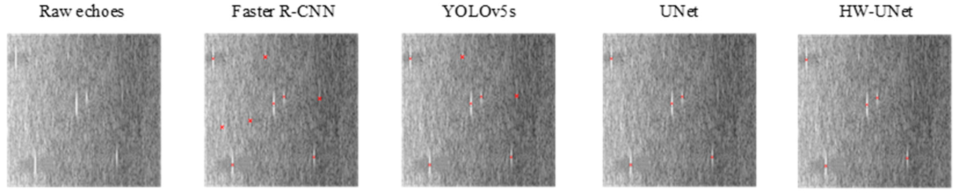
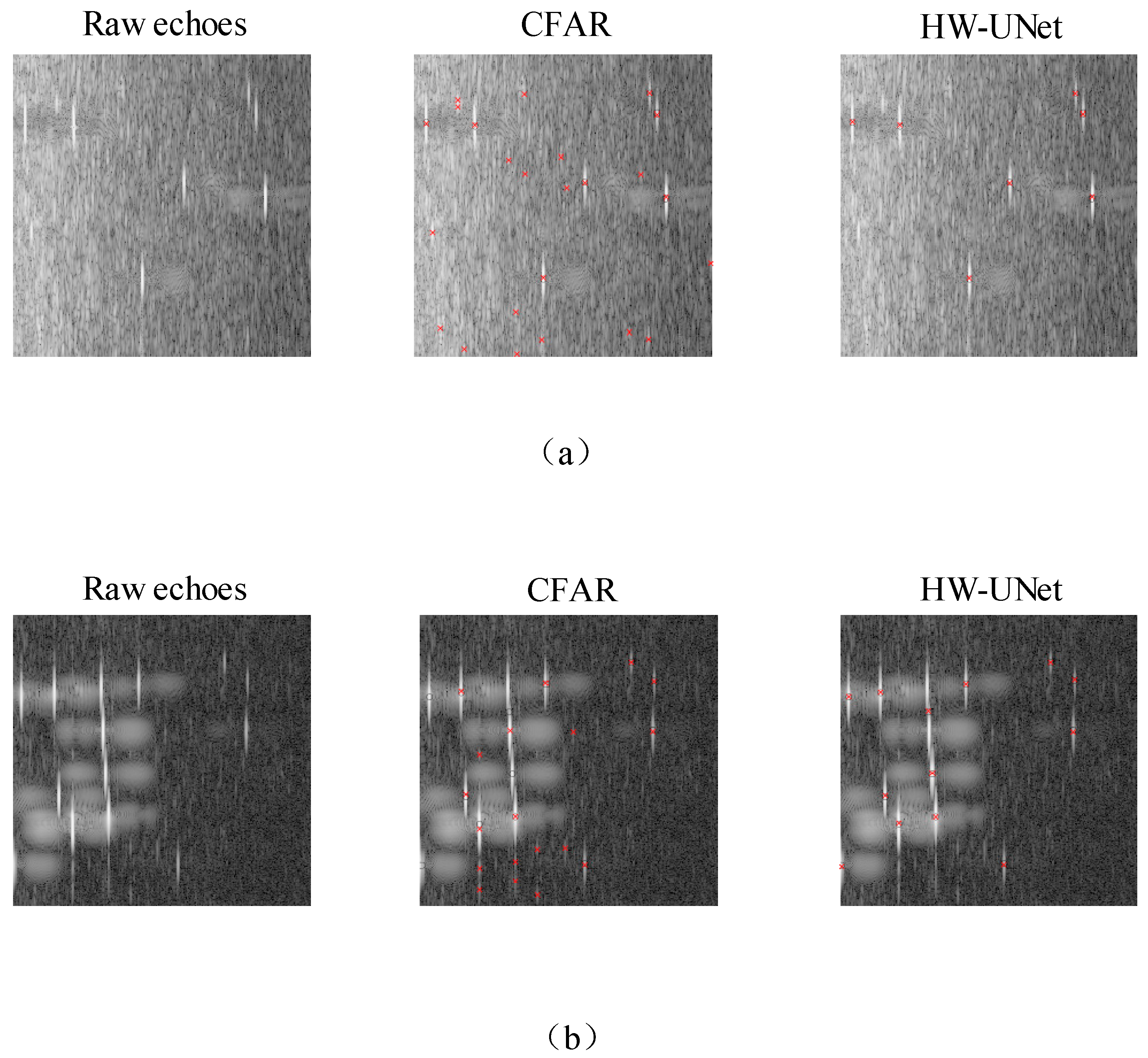
The input image resolution of the dataset was 256 × 256, with grayscale represented by 8-bit pseudo-color. The detection results of each network in a certain scene slice are shown in Figure 7. The accuracy of the network models was evaluated using the mAP metric, while the model size was assessed using the number of parameters (PA) and computational operations (OA). HW-UNet was compared with commonly used radar target-detection algorithms, including Faster R-CNN and YOLO-V5s, as well as the classical U-Net. The results are shown in

Table 1. Comparison of simulation results.

Detection Algorithms	mAP	PA (Byte)	OA (FLOPs)
Faster R-CNN [7]	75.6%	27.2 M	17.5 G
YOLOv5s [13]	80.3%	7.2 M	8.2 G
U-Net [21]	83.4%	7.76 M	10.3 G
HW-UNet	82.6%	0.52 M	1.2 G

. HW-UNet outperformed other networks in terms of comprehensive performance, achieving a better balance between accuracy and model size. In terms of accuracy, HW-UNet had higher detection accuracy than Faster R-CNN and YOLO-V5s but slightly lower than the U-Net. In terms of model size, HW-UNet used only 0.46 MB of parameters with 1.13 G FLOPs, significantly lower than other networks.

4. FPGA Design and Implementation

To deploy HW-UNet on an FPGA, further optimization is required based on the characteristics of the FPGA. This chapter first proposes the architecture of the FPGA accelerator system. By employing modular and templated design approaches, the development efficiency of the entire accelerator system is enhanced. Through network parametric design, the number of quantization bits is reduced. The network structure for the HW-UNet network adopts a hybrid layer design, which saves accelerator hardware resources and reduces the number of memory accesses. Additionally, the convolution operation, which occupies the largest proportion in the accelerator system, is optimized through intra-layer pipelining in the convolutional layer design, thereby improving the speed of convolutional computation. A pipelined parallel architecture design is also implemented to increase inference speed.

4.1. FPGA Implementation of the Acceleration Process

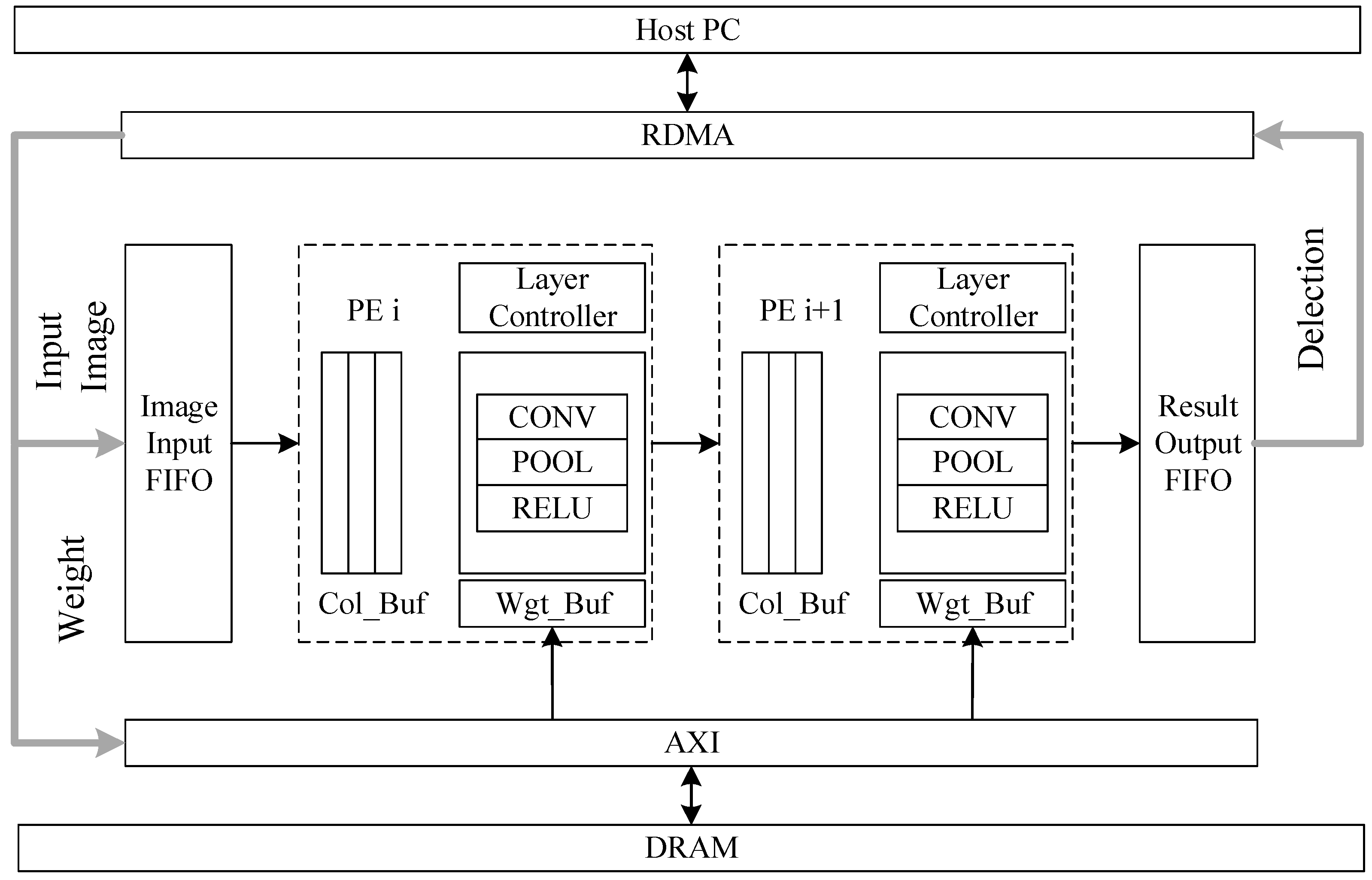
This paper adopts the system architecture proposed in [27] to implement the adaptive and acceleration process and makes improvements for practical applications. The software and hardware interaction environment as shown in Figure 8 is designed. The system is mainly composed of the peripheral data paths and the cascaded processing units Process Engine (PE) of each layer. The HOST PC is connected to the FIFO in the FPGA through the Remote direct memory access (RDMA) interface. After installing the RDMA driver, the operating system will recognize the FPGA as a network terminal device and access it through memory reading and writing. In the HOST PC, the system calls “write()”, “memcpy()” and “read()” can be utilized respectively to write input data, weights and read inference results into the FPGA through the network. Inside the FPGA, through the Advanced extensible Interface (AXI) bus, the Input and weights are sent to the Input FIFO and MIG respectively. MIG stores the weights in the off-chip DRAM through the DDR interface. During reasoning, the weights are loaded onto the on-chip input FIFO through AXI(). After the reasoning is completed, the reasoning result will be sent to RDMA through the AXI bus and then transferred to the HOST PC via RDMA.

In Figure 8, the outer data path is composed of RDMA, AXI, and MIG. RDMA communicates with the host PC via a 40 G Ethernet interface using the RDMA over Converged Ethernet (ROCE) V2 protocol for data and weight transfer. The AXI bus is responsible for on-chip data and weight distribution, while the MIG accesses off-chip DRAM through a DDR3 interface for weight transfer.

The PE is the core of the system design, incorporating various computational units used in the HW-UNet architecture, such as traditional convolution, DWC, PWC, ReLU6 activation function, and average pooling, as well as row cache and parameter FIFO cache unit designed to accelerate computation speed. PE mainly consists of the buffering units like Column_buffer and Wgt_Buffer, the Layer Controller control unit, and the computation units like CONV, POOL and RELU. The unit Column_buffer stores input data for convolutional layers, while the Wgt_Buffer caches weights. The Layer Controller is responsible for the scheduling of the PE module, and the control logic generation center decodes instructions and generates control signals for the corresponding computational modules, receiving completion signals upon finishing calculations. Data are stored in Block RAM (BRAM)-generated feature map caches, and the AXI-DataMover module ensures data interaction between the FPGA and DDR.

CNN layers, including convolutional, pooling, and fully connected layers, have corresponding weight parameters that are pre-trained using the PyTorch framework. During initialization, these weights are loaded from the Host PC into DRAM. In the inference stage, input feature maps are sent column-wise to the input FIFO via RDMA, processed through the pipeline of PEs, and the final results are sent back to the Host PC via RDMA for post-processing. The parameterized design and adaptive adder tree allow the PE to be encapsulated as an IP core, supporting different convolution sizes and configurable parallelism to balance pipeline timing. On-chip memory (Block RAM, distributed RAM, or ultra RAM) is divided into multiple banks for caching features, weights, and bias data. When the accelerator starts a layer, these data are loaded from off-chip memory into the corresponding on-chip memory. If sufficient data are available, the engine reads the input, performs calculations, and writes the results back to memory. Finally, the results are saved to off-chip memory.

The Host PC can transmit control instructions via RDMA, enhancing the convenience of debugging. The radar target-detection accelerator can also operate independently of the PC by pre-storing weight parameters in the FPGA’s internal memory, with diverse output options (e.g., high-speed bus or hardware display panel).

4.2. Fine-Grained Network Parameter Quantization

The parameters of CNNs are generally represented using floating-point numbers, ensuring the model’s precision, thereby enhancing the accuracy of target detection. The high-precision representation method requires high-performance computational resources. With its exceptional parallel processing capabilities, GPU has become the preferred hardware for training complex CNN models, effectively handling large-scale data and intricate computational tasks. However, when these high-precision models are deployed onto FPGAs, the use of floating-point numbers consumes significant hardware resources. In such cases, quantization methods are employed to convert floating-point numbers into low-precision fixed-point numbers. This effectively reduces the model’s demand for storage resources and lowers computational complexity, thereby enabling CNN models to operate efficiently on resource-constrained devices.

Quantizing 32-bit floating-point numbers to 8-bit fixed-point numbers (INT8) reduces model size to one-fourth of its original, thereby significantly decreasing memory occupancy. Faster memory data access enables algorithm acceleration.

However, simple INT8 quantization may result in significant precision loss, limiting its applicability. To address this, we employ a shift-based quantization method targeting single-layer network activation and weight data. This method avoids large quantization steps caused by varying data ranges across layers, maintaining zero values and simplifying activation operations. The quantization bit-width can be customized to balance precision and speed. In this work, we adopt a 16-bit activation and 8-bit weight quantization scheme (16-8 bit quantization) to achieve a good trade-off. The quantization process is defined by the following Equations (11)–(13), as follows:

$$s={\log }_{2}Max(\left|q_{\max }\right|,\left|q_{\min }\right|)$$

(11)

$$k=2^{w-1}$$

(12)

$$q=\left[r\times k\right]$$

(13)

where r is the original floating-point parameter; w is the data bit-width (16 or 8); k is the scaling factor; and q is the quantized integer, representing a fixed-point number.

Using this method, the volume of activation and weight data is reduced by half compared to the original float32 format, with less than 1% precision loss. This balance between speed and precision is crucial for efficient inference in resource-constrained environments.

4.3. Mixed Layer Design

Batch normalization (BN) is a technique used to accelerate the inference of neural networks. The primary functions of BN layers include normalizing the output distribution of each network layer, alleviating internal covariate shift, accelerating the convergence speed of the training process, preventing saturation of activation functions and abnormal increases in gradients, enhancing the generalization capability of the model, and increasing the independence between different layers of the network. However, during the forward inference process, BN layers transition from training mode to testing mode, utilizing fixed mean and variance values obtained after model training. Therefore, integrating BN layers into convolutional computations can save the resource overhead of BN layers, especially in FPGA hardware implementations, where there is no need to design a separate hardware circuit for BN operations. Moreover, BN layer integration can also accelerate the inference speed of the network.

During the computation process, a normalization layer and an activation function layer are added after each convolutional layer operation. In this context, layer fusion technology is introduced for this type of structure. Since BN layers can degrade model performance during inference, BN layers can be integrated into the convolutional layers through layer fusion during the inference process, thereby reducing the computational load and enhancing model performance. The layer fusion process is described below.

Layer fusion technology integrates the data from convolutional layers, normalization layers, and activation function layers into a single layer. This reduces the number of data exchanges from three to one, without introducing additional computational load. In the network used in this design, the normalization layer is mainly responsible for data translation operations. Based on the computational characteristics of the normalization layer, it can be fused with the other two layers, as shown in Equation (14).

$$y_i=\gamma {\displaystyle \frac{x_i-\mu }{\sqrt{{\delta }^2+\epsilon }}}+\beta$$

(14)

In Equation (14), $\mu$ represents the mean of a batch, ${\delta }^2$ represents the standard deviation of a batch, and $\epsilon$ is a very small constant to avoid the abnormal situation where the ${\delta }^2$ is zero.

γ and β are learnable parameters. During training, like other convolutional kernel parameters, they are learned through gradient descent. Here, γ is the scale factor, and β is the shift factor. The scale factor optimizes the width of the feature data distribution, while the shift factor optimizes the offset of the data. These two parameters are automatically learned during model training and their values are fixed after training. Expanding Equation (15), as follows:

$$y_i=\gamma {\displaystyle \frac{x_i-\mu }{\sqrt{{\delta }^2+\epsilon }}}+\beta ={\displaystyle \frac{\gamma }{\sqrt{{\delta }^2+\epsilon }}}{x}_i+(\beta -{\displaystyle \frac{\gamma \mu }{\sqrt{{\delta }^2+\epsilon }}})$$

(15)

The formula is simplified by letting $a={\displaystyle \frac{\gamma }{\sqrt{{\delta }^2+\epsilon }}}$, $b=\beta -{\displaystyle \frac{\gamma \mu }{\sqrt{{\delta }^2+\epsilon }}}$ obtain Equation (16), as follows:

$$y_i=a{x}_i+b$$

(16)

Thus, it can be concluded that BN is a linear operation, which is essentially a scaling operation followed by a shifting operation. This linear operation can be integrated into the preceding fully connected layer or convolutional layer.

The convolution formula incorporating BN can be defined as in Equation (17), as follows:

$$x_i=w_{conv}\times z_i+b_{conv}$$

(17)

$x_i$ represents the input to the BN; $z_i$ represents the input to the conv; $w_{conv}$ represents the weights of the convolutional layer; and $b_{conv}$ represents the bias of the convolutional layer. Substituting these into Equation (18) yields

$$y_i={\displaystyle \frac{\gamma }{\sqrt{{\delta }^2+\epsilon }}}(w_{conv}\times z_i+b_{conv})+\beta -{\displaystyle \frac{\gamma \times \mu }{\sqrt{{\delta }^2+\epsilon }}}$$

(18)

Expanding the content within the parentheses of Equation (18) results in Equation (19), as follows:

$$y_i={\displaystyle \frac{\gamma \times w_{conv}}{\sqrt{{\delta }^2+\epsilon }}}(z_i)+{\displaystyle \frac{\gamma \times b_{conv}}{\sqrt{{\delta }^2+\epsilon }}}+\beta -{\displaystyle \frac{\gamma \times \mu }{\sqrt{{\delta }^2+\epsilon }}}$$

(19)

In Equation (19), ${\displaystyle \frac{\gamma \times w_{conv}}{\sqrt{{\delta }^2+\epsilon }}}$ represents the new weights after the integration of Conv and BN, ${\displaystyle \frac{\gamma \times (b_{conv}-\mu )}{\sqrt{{\delta }^2+\epsilon }}}+\beta$ represents the new bias after the integration of Conv and BN.

The transformation of parameters w and b primarily relies on incorporating the pre-trained parameters (γ, β) to calculate the new convolution kernels and biases in advance. After performing this substitution, the convolution function with layer fusion can replace the traditional convolution function. This operation does not introduce new multiplicative or additive calculations during convolution but reduces data transfer by replacing multiple data transfers with a single one, thereby improving the efficiency of memory access. The fused layer effectively reduces the computational load during model inference on the FPGA, decreasing the consumption of on-chip FPGA resources such as Digital Signal Processing (DSP) and Look Up Table (LUT). Additionally, since the number of computational steps is reduced, inference latency is also decreased to some extent, enhancing the overall system performance.

4.4. FPGA Implementation-Optimization Methods

This design utilizes the FPGA in a heterogeneous platform as an external acceleration device to accelerate neural network inference. Among the optimization strategies for FPGA acceleration, two methods are particularly effective. The first is to reduce the number of data transfers by optimizing data-transmission strategies to minimize access to external memory and reduce I/O time. The second is to minimize the number of multiplication and addition operations during computation by employing a space-for-time strategy to reduce the computational load. This design incorporates multi-level pipelining and multi-channel parallel convolution to optimize memory-access efficiency and improve the utilization of computational resources, ultimately achieving reduced hardware-resource usage and ease of implementation.

4.4.1. Multi-Level Pipelining

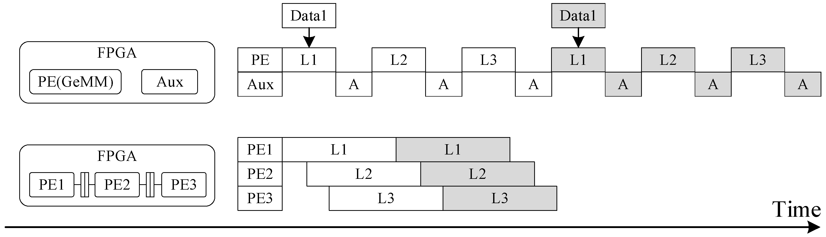
Among the optimization strategies mentioned above, in addition to the optimization of data transmission to enhance computational speed, another space-for-time approach to accelerate computation involves introducing multi-level pipelining. This is a common operator-acceleration strategy used on FPGAs.

In this design, convolution operators, which are the most computationally intensive, are targeted for optimization. Therefore, a hybrid-granularity multi-level pipelining architecture is introduced and then coupled with dataflow and parallelism design to eliminate pipeline bubbles and optimize convolutional-layer computations. For example, in the improved inverted residual structure shown in Figure 3c, L1 represents a 3 × 3 DWC block computation, L2 represents a 1 × 1 convolution block computation, and L3 represents another 3 × 3 DWC computation. Originally, L1, L2, and L3 convolutions are executed in parallel. Through the implementation of a pipelined strategy for the L1, L2, and L3 convolution circuits, data exchanges with external memory during computation are reduced, thereby improving computational efficiency. A comparison of the specific processes is shown in Figure 9.

4.4.2. Multi-Channel Parallelism

During the hardware design of the convolution operator, this design employs a strategy of multi-channel parallel convolution computation. First, compared to single-channel convolution, multi-channel parallel computation significantly improves computational efficiency and accelerates the inference process of the network. Multi-channel parallel computation can more effectively utilize the computational and storage resources on the FPGA, greatly improving resource-utilization efficiency through this parallelized design. Given the high flexibility of FPGAs, parallel-processing units and data-transfer strategies can be designed according to application requirements. The degree of parallelism can be flexibly configured based on the size of the input feature maps and network parameters to achieve optimal performance. After the multi-channel parallel convolution strategy has been introduced, data can be processed in multiple local channels, further reducing access to external memory, thereby reducing memory-access latency and accelerating data processing speed.

5. Experimental Results and Analysis

5.1. Experimental Environment

The Xilinx Kintex UltraScale FPGA-based KCU1500 acceleration-development kit was selected as the system-implementation platform, as shown in Figure 10. The KCU1500 employs the Kintex UltraScale architecture, which is specifically designed for large-scale application development. It supports PCIe Gen3 interfaces and features two Quad Small Form-factor Pluggable (QSFP) modules. Equipped with 16 GB DDR4 memory supporting Error-Correcting Code (ECC) functionality, the board also includes 1 Gb Dual Quad Serial Peripheral Interface (SPI )Flash storage. The board supports dynamic modification of logic blocks without the need for full reconfiguration. The development environment utilizes the Vivado Design Suite and HLS.

Real-time radar data streams at 5 Mbps were received through QSFP fiber interfaces in the experiment. The acceleration task was completed through a co-processing approach between hardware and software on the CPU side. The complete convolution accelerator was designed and implemented based on the Vivado Design Suite, with key modules of the convolution accelerator designed using HLS and corresponding IP cores generated.

5.2. Hardware-Resource Utilization and Computational Speed

After the functional module design had been completed on the FPGA, synthesis and place-and-route processes were performed. Vivado automatically provided detailed resource-utilization statistics, as shown in

Table 2. Hardware-resource utilization.

Resource	LUT	Distributed RAM	Flip-Flops	DSP Slices	BRAM
Total	663,360	18,360	1,326,720	5520	2160
Usage	231,084	3762	421,440	2496	435
Percentage	34.8%	20.5%	31.8%	45.2%	20.1%

. The results indicated that DSP slices had the highest utilization rate at 45.2%, primarily due to the 128 parallel convolution windows used in the convolution calculation module. LUTs were mainly used for addition and shift operations, with 231,084 utilized. Distributed RAM was used for linear buffering, Flip-Flops served as registers, and BRAM was used for caching input feature blocks, weight data, intermediate results, and output feature blocks. Except for the DSP slices, the utilization rates of all resources were below 40%, indicating efficient resource utilization and conservation of hardware resources.

According to the test plan, the accelerator card received radar data in real time through fiber optics and performs network model inference via the FPGA, ultimately completing the experimental test. Through this experiment, under a 200 MHz working clock, the HW-UNet FPGA accelerator achieved real-time radar target detection with a data stream of 7.2 Mbps. The data showed that the HW-UNet network model FPGA accelerator achieved real-time radar target detection with a data stream of 5 Mbps and was faster than this index.

5.3. HW-UNet Target-Detection Results

In specific slice scenarios with strong sea clutter and multi-target environments, the detection performance of HW-UNet was compared with that of the traditional CFAR detection method, as shown in Figure 11. The statistical results were presented in

Table 3. Comparison of detection results between CFAR and HW-UNet in sliced scenarios.

Scenarios	Number of True Targets	Number of True Targets CA-CFAR	Number of False Targets CA-CFAR	Number of True Targets HW-UNet	Number of False Targets HW-UNet
Strong clutter	7	7	17	7	0
Multi-target clutter	14	9	9	13	0

. The experimental results indicated that while the CFAR method could detect small targets in the scenario, it generated a significant number of false alarms across all scenarios. Moreover, in multi-target scenarios, CFAR was prone to missing detections due to mutual interference between targets, clutter peaks, and sidelobes. By contrast, the HW-UNet method achieved an average detection rate of 95.24% without any false alarms in the same scenario. Through long-term statistical analysis of a large number of data samples, under the same detection-probability condition (0.001), the target-detection probability for CFAR was 78.3%, while for HW-UNet, it was 85.6%. These experimental data demonstrated that HW-UNet had a stronger target-detection capability compared to the CFAR method.

6. Discussion

This paper proposes a radar sea-surface target-detection accelerator design, employing techniques such as DSC, inverted residual structures, and ASPP to optimize the U-Net network. These improvements effectively reduce the number of network parameters and the computational load. Additionally, the design incorporates a flexible implementation framework based on RDMA, fine-grained network parameter quantization, and parallel pipelining to minimize FPGA resource usage and enhance processing efficiency. Experimental results demonstrate that the HW-UNet accelerator, due to quantization of parameters and computational results on the FPGA, experiences a slight drop in average detection accuracy compared to GPU implementations. However, the precision loss is less than 1%, which places it within an acceptable range. In sea-clutter environments, traditional CA-CFAR algorithms are prone to false detections of sea-clutter peaks as targets and are more likely to miss detections in multi-target scenarios due to mutual interference between targets, clutter peaks, and sidelobes. In contrast, the deep learning algorithm based on HW-UNet learns from the tendencies of human annotators in the ground-truth labels, effectively suppressing sea clutter while maintaining a high level of target-detection capability.

The HW-UNet network addresses the challenge of deploying radar target detection on FPGA with limited resources, achieving real-time target-detection processing of radar data streams at 7.2 Mbps without compromising detection accuracy. Future work will focus on further increasing parallelism in layer-by-layer convolution processing to improve throughput and handle higher radar data rates. Additionally, training and validating the accelerator with datasets from various radar scenarios will enhance its generalization capability for radar target detection. In particular, we aim to optimize the network to handle even higher data rates and improve its robustness in diverse maritime environments.