Robust 12-Lead ECG Classification with Lightweight ResNet: An Adaptive Second-Order Learning Rate Optimization Approach

Abstract

To enhance the classification accuracy of the ResNet model for 12-lead ECG signals, a novel approach that focuses on optimizing the learning rate within the model training algorithm is proposed. Firstly, a Taylor expansion of the training formula for model weights is performed to derive a learning rate that incorporates the second-order gradient information. Subsequently, to circumvent the direct computation of the complex second-order gradient in the learning rate, an approximation method utilizing the historical first-order gradient is introduced. Additionally, truncation techniques are employed to ensure that the second-order learning rate remains neither excessively large nor too small. Ultimately, the 1D-ResNet-AdaSOM model is constructed based on this adaptive second-order momentum (AdaSOM) method and applied for 12-lead ECG classification. The proposed algorithm and model were validated on the CPSC2018 dataset. The evolving trend of the loss function throughout the training process demonstrated that the proposed algorithm exhibited commendable convergence and stability, and these results aligned with the conclusions derived from the theoretical analysis of the algorithm’s convergence. On the test set, the model attained an impressive average F1 score of 0.862, demonstrating that 1D-ResNet-AdaSOM surpassed several state-of-the-art deep-learning models in performance while exhibiting strong robustness. The experimental findings further substantiate our hypothesis that adjusting the learning rate in the ResNet training algorithm can effectively enhance classification accuracy for 12-lead ECGs.

1. Introduction

The 12-lead electrocardiogram (ECG) signals, which yield a more comprehensive understanding of cardiac activity, represent a non-invasive, cost-effective method for cardiac health screening and have found extensive applications in clinical diagnostics. Nevertheless, the signals derived from these twelve leads exhibit considerable variability [1]. Consequently, the analysis of these intricate ECG signals poses a significant challenge for clinicians due to their time-consuming nature. Employing artificial intelligence and machine learning techniques to facilitate the analysis of 12-lead ECGs emerges as an efficacious solution to address this pressing issue [2,3,4].

Currently, various traditional machine learning methods have been employed for ECG classification, including naïve Bayes (NB) [5], k-nearest neighbors (KNNs) [6], support vector machines (SVMs) [7], logistic regression [8], random forests (RFs) [9], extreme learning machines (ELMs) [10], and artificial neural networks (ANNs) [11]. The general procedure for ECG classification using these traditional machine learning techniques consists of several key steps: preprocessing the ECG signals, extracting features from the ECG data, training machine learning models, and predicting the categories of the samples. Among these steps, feature extraction from ECG signals is particularly critical and challenging. This process involves various techniques, such as the medical characterization of ECGs [12] and both the time-domain and frequency-domain analyses of ECG signals [13,14].

In recent years, deep learning has achieved significant success in the field of image recognition [15]. Numerous studies have also demonstrated that ECG signals can be treated as one-dimensional images and recognized with deep-learning models [16]. In [17], a one-dimensional convolutional neural network (1D-CNN) is employed to automatically extract features from ECG images through convolutional, pooling, dropout, and normalization layers. Ultimately, the Adam optimization algorithm is utilized to train the model. In [18], an approach is proposed that leverages the LSTM model and auto-encoder for feature extraction from ECG signals; subsequently, the SVM is used to classify these signals based on the learned features. In [19], DenseNet, a developed CNN model, is employed to extract features from ECG signals. Additionally, refs. [20] suggest that deep-learning models utilizing ResNet and Inception architectures demonstrate remarkable performance in the recognition of 12-lead electrocardiograms. From the aforementioned literature, it becomes evident that enhancing the accuracy of deep-learning models for 12-lead ECG classification primarily focuses on deep feature extraction techniques. Deep-learning models typically consist of two main components: deep feature extraction and deep feature learning; however, there is limited literature addressing methods to improve classification accuracy during the deep feature learning phase, specifically for ECG data. To address this gap, this paper adopts 1D-ResNet as the foundational deep-learning model for ECG classification [20,21] and investigates strategies to enhance its classification accuracy within the 1D-ResNet’s deep feature learning process. The principal contributions of this paper are summarized as follows: (1) A novel training algorithm for the 1D-ResNet model, designed to enhance the classification accuracy of 12-lead ECG signals, is proposed in this study. Traditional deep-learning models for ECG classification typically utilize complex deep feature extraction methods to improve accuracy, which inevitably increases model complexity and design challenges. In contrast to conventional approaches, our method enhances classification accuracy by optimizing the learning rate within the training algorithm without altering the architecture of the deep-learning model. Consequently, the proposed model maintains a lightweight architecture compared to traditional ECG deep-learning frameworks while achieving competitive performance. (2) A momentum method incorporating a second-order learning rate is proposed to enhance the classification accuracy of 1D-ResNet for ECG classification. Based on the weight training model of 1D-ResNet, the learning rate with second-order gradient information is derived. To mitigate the challenges associated with directly computing the second-order gradient information in the learning rate, a method of approximating the second-order learning rate with the historical first-order gradient is introduced. Furthermore, truncation techniques are employed to ensure that the second-order learning rate remains within appropriate bounds, preventing excessive oscillations during the iterative process. The designed second-order learning rate is capable of adapting to the current momentum, facilitating the acquisition of high-quality weights and thereby improving ECG classification accuracy for 1D-ResNet. (3) Experiments were conducted on the CPSC2018 dataset, which included noise. The convergence performance of the proposed training algorithm was evaluated in comparison to classical training algorithms. Additionally, the classification results of 12-lead ECG signals produced by the proposed model were compared with those of state-of-the-art competing deep-learning models. The experimental results confirm both the effectiveness and superiority of the proposed algorithm and model.

This paper is organized as follows: Section 2 provides a summary of the related work pertinent to this research. Section 3 offers a detailed description of the momentum method utilizing a second-order learning rate. In Section 4, the convergence analysis of the proposed momentum method is presented. Section 5 demonstrates the feasibility and effectiveness of the proposed algorithm and model through experiments. Finally, Section 6 concludes with a summary of the entire paper.

2. Related Work

Figure 1 depicts the architecture of a 1D-ResNet-34 model designed for the ECG signal recognition [20,21,22]. This model comprises a total of 34 layers. The Conv1D layer executes convolutional operations on the input one-dimensional ECG signals, facilitating both data transformation and feature extraction. The BatchNorm1D layer normalizes these features to mitigate the sensitivity of the ResNet model to variations in input data distribution. The ReLU layer applies nonlinear transformations to the input data, and the pooling layer performs downsampling on features, thereby reducing their dimensionality while preserving essential information. The residual blocks employ skip connections as a technique to address issues related to vanishing or exploding gradients. The output from these residual blocks is subsequently downsampled by the pooling layer, yielding the deep features of the ECG signals. Finally, the dense layer, commonly referred to as the fully connected layer, integrates and transforms deep features; it subsequently maps and outputs the categories of the ECG samples through the built-in Softmax function, thereby achieving the classification and identification of ECG signals. In summary, in the 1D-ResNet-34 model, the first 33 layers are responsible for extracting deep features, and the final dense layer is for the classification and recognition of these deep features.

For the $i$-th ECG training sample, its true label is denoted as $y_i$; the deep feature vector extracted by 1D-ResNet to $y_i$ is denoted as $x_i$, and the predicted label for $x_i$ is denoted as ${\widehat{y}}_i$. The cross-entropy function is used as the training loss function of 1D-ResNet, which is defined as

$$f\left(w\right)=-{\displaystyle \frac{1}{N}}{\displaystyle \sum _{i=1}^N{\displaystyle \sum _{k=1}^K{y}_{i,k}\log {\widehat{y}}_{i,k}}}$$

(1)

where $N$ represents the number of training samples, while $K$ denotes the number of categories. The weights of 1D-ResNet are denoted as $w$. The term $y_{i,k}$ indicates the value of the $k$-th dimension of the true label for the $i$-th sample, and ${\widehat{y}}_{i,k}$ signifies the value of the $k$-th dimension of the predicted label for the $i$-th sample. $f(w)$ reflects the degree to which the predicted labels in the training set diverge from their corresponding true labels.

The predicted label ${\widehat{y}}_i$ in Equation (1) can be interpreted as the output of the implicit function $p(\cdot )$, expressed as ${\widehat{y}}_i=p\left(x_i,w\right)$. Consequently, ${\widehat{y}}_i$ is dependent on $w$. The training process for 1D-ResNet involves determining the optimal weights $w$ that align with the deep features extracted from the training set through an optimization algorithm, aiming to minimize the loss function $f(w)$. Consequently, this training procedure can be formulated as an unconstrained optimization problem:

$$\underset{w\in {ℝ}^D}{\min }f\left(w\right)$$

(2)

where $f(w)$ is continuously differentiable.

For the optimization problem described in Equation (2), the momentum method [23], which is based on first-order gradients or its variants, is widely employed for its resolution. The iterative solution formula utilized in the momentum method is given as follows [24].

$$d_t=\beta d_{t-1}+\left(1-\beta \right)g_t$$

(3)

$$w_{t+1}=w_t+{\alpha }_t{d}_t$$

(4)

where $t$ represents the number of iterations, and $w_t$ denotes the weights at the $t$-th iteration. Let $g_t=-\nabla f(w_t)$ denote the first-order stochastic negative gradient of $f(w)$ at $w_t$. Additionally, let $d_t$ and $d_{t-1}$ represent the update directions for the parameter $w$ at the current $t$-th and previous ($t$ − 1)th iterations, respectively. The term $\beta$, known as the momentum coefficient, lies within the range of [0, 1), controlling the extent to which historical gradient contributions influence current updates. The learning rate denoted by ${\alpha }_t>0$ is typically maintained as a constant in momentum methods to simplify algorithmic complexity. Equation (3) can be interpreted as the synthesis of a new negative gradient, denoted as $d_t$, which incorporates both the historical negative gradient, $d_{t-1}$, and the current negative gradient, $g_t$. This approach aims to mitigate oscillations during iterations described in Equation (4).

Problem (2) can be addressed utilizing the Adam algorithm too, which employs the following iterative formula [25]:

$$w_{t+1}=w_t+{\alpha }_t{d}_t/(\sqrt{v_t}+\epsilon )$$

(5)

where ${\alpha }_t$ is the learning rate. The term $v_t$ represents the estimate of the second raw moment. When considering ${\alpha }_t/(\sqrt{v_t}+\epsilon )$ as the dynamic learning rate, it encompasses momentum information and adapts to the current momentum $d_t$. Motivated by this observation, we propose a novel adaptive learning rate that integrates second-order gradient information to enhance both the convergence speed and stability of Equation (4).

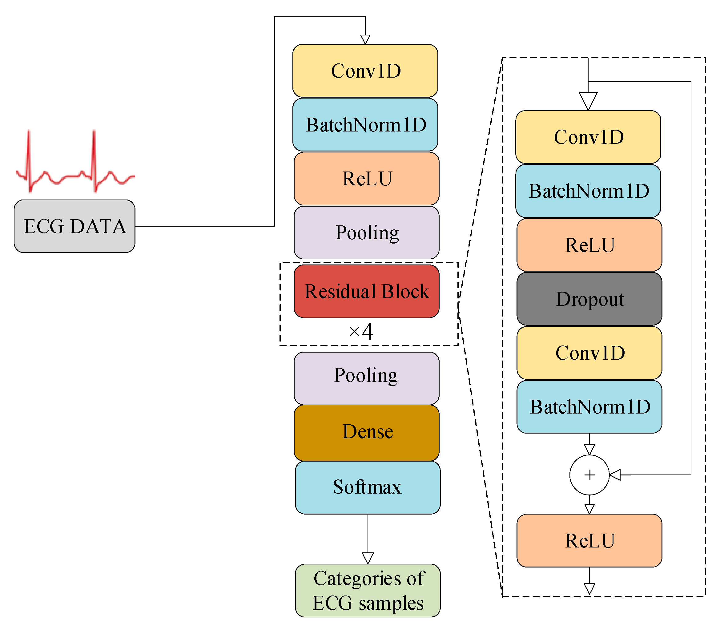
3. Adaptive Second-Order Momentum Method (AdaSOM)

The cross-entropy loss function $f(w)$, as described in Equation (1), exhibits quadratic differentiability. In accordance with Equation (4), a Taylor expansion of $f(w_t)=f(w_{t-1}+{\alpha }_{t-1}{d}_{t-1})$ is derived, incorporating quadratic terms as follows.

$$f\left(w_{t-1}+{\alpha }_{t-1}{d}_{t-1}\right)\approx f\left(w_{t-1}\right)+{\alpha }_{t-1}\left(\nabla f\left(w_{t-1}\right)\odot d_{t-1}\right)+{\displaystyle \frac{{\alpha }_{t-1}^2}{2}}\left(\left({\nabla }^{2}f\left(w_{t-1}\right)d_{t-1}\right)\odot d_{t-1}\right)$$

(6)

where ⊙ denotes the inner product operation of vectors. The term ${\nabla }^{2}f(w_{t-1})$, which contains second-order gradient information, represents the Hessian matrix of the function $f(w_{t-1})$, evaluated at $w_{t-1}$. If the curvature term $\left({\nabla }^{2}f\left(w_{t-1}\right)d_{t-1}\right)\odot d_{t-1}$ is positive, there exists a unique value $\alpha (w_{t-1})$ in Equation (6) that minimizes $f\left(w_{t-1}+{\alpha }_{t-1}{d}_{t-1}\right)$. Here, to simplify the calculation, let $d_{t-1}=-\nabla f\left(w_{t-1}\right)$; therefore, $\alpha (w_{t-1})$ can be calculated using the following formula [26,27]:

$$\alpha (w_{t-1})={\displaystyle \frac{{‖\nabla f\left(w_{t-1}\right)‖}^2}{\left({\nabla }^{2}f\left(w_{t-1}\right)\nabla f\left(w_{t-1}\right)\right)\odot \nabla f\left(w_{t-1}\right)}}$$

(7)

where the learning rate $\alpha (w_{t-1})$ in Equation (7) is computed using the second-order gradient information ${\nabla }^{2}f(w_{t-1})$. The notation ||⋅|| denotes the 2-norm operation on vectors, yielding a scalar result. Accurately calculating the Hessian matrix for large-scale problems poses significant challenges; therefore, in this paper, the first-order gradient information is used to approximate the Hessian matrix, thereby enhancing the computational efficiency. This approximation is derived from the iterative formula $w_t=w_{t-1}-{\alpha }_{t-1}\nabla f(w_{t-1})$ and Taylor’s theorem:

$$\mathsf{\Delta }{w}_t=w_t-w_{t-1}=-{\alpha }_{t-1}\nabla f\left(w_{t-1}\right)$$

(8)

$$\mathsf{\Delta }{g}_t=\nabla f\left(w_t\right)-\nabla f\left(w_{t-1}\right)\simeq -{\alpha }_{t-1}{C}_f\left(w_{t-1}\right)$$

(9)

where $C_f\left(w_{t-1}\right)={\nabla }^{2}f(w_{t-1})\nabla f(w_{t-1})$.

By reformulating Equation (7) in terms of Equations (8) and (9), the learning rate associated with the adaptive second-order information can be derived as follows.

$${\alpha }_t^{*}\simeq \alpha \left(w_{t-1}\right)=\frac{{\left|\right|\mathsf{\Delta }{w}_t\left|\right|}^2}{\mathsf{\Delta }{w}_t\odot \mathsf{\Delta }{g}_t}$$

(10)

The learning rate ${\alpha }_t^{*}$ derived from Equation (10) may be excessively large or small, potentially leading to instability during the iteration process. In [26], a solution was proposed: for a parameter of $\eta >0$, when $‖{\alpha }_t^{*},g_t‖>\eta$, the learning rate is adjusted to $\eta /‖g_t‖$ to ensure that $‖w_{t+1}-w_t‖=\eta$; otherwise, the learning rate remains as ${\alpha }_t^{*}$, in which case it holds that $‖w_{t+1}-w_t‖\le \eta$. Inspired by this approach, in this paper, the value of $\eta$ is defined as $‖w_{t+1}-w_t‖$, and a boundary learning rate ${\mu }_{\mathrm{t}}$ is constructed to solve the problem of an overly large learning rate. Additionally, a scalar $\gamma >0$ is defined to prevent the learning rate from being too small, thereby obtaining a new corrected learning rate, whose corresponding computational equations are formulated as follows.

$${\mu }_t={\displaystyle \frac{\eta }{‖g_t‖}}$$

(11)

$${\widehat{\alpha }}_t=\max \left(\gamma ,\min \left({\alpha }_t^{*},{\mu }_t\right)\right)$$

(12)

The max(∙) function is designed to ensure that when $\left({\nabla }^{2}f(w_{t-1})d_{t-1}\right)\odot d_{t-1}$ is negative, the resulting learning rate remains non-negative. Equation (12) employs min(∙) and max(∙) as truncation techniques to prevent the learning rate from becoming excessively large or too small.

In the original momentum method, the value of $d_t$ derived from the initial computation may be relatively small, leading to a significant bias in parameter updates during the early stages of training. To mitigate this bias, $d_t$ is adjusted for initialization bias through the following correction method.

$${\widehat{d}}_t={\displaystyle \frac{d_t}{1-{\beta }^{t+1}}}$$

(13)

Reformulating Equation (4) in conjunction with Equations (12) and (13) results in the iterative solution equation for AdaSOM applied to address Problem (2), as demonstrated below.

$$w_{t+1}=w_t+{\widehat{\alpha }}_t{\widehat{d}}_t$$

(14)

Based on the equations above, the algorithmic steps of AdaSOM for training the 1D-ResNet are outlined as follows (Algorithm 1).

Algorithm 1. AdaSOM.

1: Input: maximum iterations $T$, learning rate ${\alpha }_0$, scalar learning rate $\gamma >0$, momentum coefficient $\beta \in [0,1)$, loss function $f(w)$, training set, and validation set. 2: Initial: $w_0$, $t\leftarrow 0$, $d_0\leftarrow 0$. 3: $w_1\leftarrow w_0-{\alpha }_0\nabla f\left(w_0\right)$. 4: $\eta \leftarrow ‖w_1-w_0‖$. 5: $t\leftarrow t+1$. 6: while $w_t$ not converged do 7:       $g_t\leftarrow -\nabla f\left(w_t\right)$. 8:       $d_t\leftarrow \beta d_{t-1}+(1-\beta )g_t$. 9:       $\widehat{d_t}\leftarrow {\displaystyle \frac{d_t}{1-{\beta }^{t+1}}}$. 10:     $\Delta w_t\leftarrow w_t-w_{t-1}$. 11:     $\Delta g_t\leftarrow \nabla f(w_t)-\nabla f(w_{t-1})$. 12:     ${\alpha }_t^{*}\leftarrow {\displaystyle \frac{{‖\Delta w_t‖}^2}{\Delta w_t\odot \Delta g_t}}$. 13:     ${\mu }_t\leftarrow {\displaystyle \frac{\eta }{‖g_t‖}}$. 14:     ${\widehat{\alpha }}_t\leftarrow \max \left(\gamma ,\min \left({\alpha }_t^{*},{\mu }_t\right)\right)$. 15:     $w_{t+1}\leftarrow w_t+{\widehat{\alpha }}_t{\widehat{d}}_t$. 16:     $\eta \leftarrow ‖w_{t+1}-w_t‖$. 17:     $t\leftarrow t+1$. 18: end while 19: return $w_t^{*}\leftarrow w_{t+1}$.

4. Convergence Analysis of AdaSOM Algorithm

Let $\mathbb{E}[\cdot ]$ denote the expectation of the potential probability space to analyze the convergence of the AdaSOM algorithm. Since the objective function $f(w)$ is continuous and differentiable, the gradient of $f$ is locally L-Lipschitz continuous. The convergence of the AdaSOM algorithm is analyzed by introducing the following three lemmas [27].

Lemma 1.

For $w_1,w_2\in {ℝ}^D$, there exists $L>0$, such that

$$\left|\right|\nabla f(w_1)-\nabla f(w_2)\left|\right|\le L\left|\right|w_1-w_2\left|\right|$$

(15)

Lemma 2.

The function $f:{ℝ}^D\to ℝ$ has an L-Lipschitz continuous gradient, and for any $w\in {ℝ}^D$ as well as $d\in {ℝ}^D$ , there exists $L>0$, satisfying the following equation:

$$f(w+d)\le f(w)+\nabla f(w)\odot d+{\displaystyle \frac{L}{2}}{‖d‖}^2$$

(16)

Lemma 3.

Let$$and $\gamma >m$. The learning rate of the AdaSOM algorithm is ${\widehat{\alpha }}_t=\max (\gamma ,\min ({\alpha }_t^{*},{\mu }_t))$. Let ${\alpha }_t=b{\widehat{\alpha }}_t{(t+1)}^{-(1/2+\delta )}$, there exists ${\alpha }_t\in [bm/{(t+1)}^{-(1/2+\delta )}$,$bM/{(t+1)}^{-(1/2+\delta )}]$.

Theorem 1.

Let $w_0\in {ℝ}^D$. ${(w_T)}_{T\in \mathbb{N}/2}$ is the sequence generated by the AdaSOM algorithm at the initial point $w_0$, and there exists a constant $C_1>0$ such that $‖w_t‖<C_1$; then, the sequence ${(f\nabla (w_T))}_{T\in \mathbb{N}}$ almost necessarily converges, and the sequence ${({\Vert f(w_T)\Vert }^2)}_{T\in \mathbb{N}}$ almost necessarily converges to 0. There exists a constant $C_2>0$ such that ${‖\nabla f(w_t)‖}^2\le C_2$, and there is

$$\underset{t\in \left\{0,\dots ,T-1\right\}}{\min }\mathbb{E}\left[{‖\nabla f(w_t)‖}^2\right]=O\left({\displaystyle \frac{1}{T^{1/2-\delta }}}\right)$$

(17)

Proof. 

For $t\in N$, $\nabla f(w_{t+1})-\nabla f(w_t)$ is restricted by using the descending direction $d=-{\alpha }_t\nabla f(w_t)$. According to Lemma 2, it can be derived that

$$f(w_{t+{\displaystyle \frac{1}{2}}})\le f(w_t)-{\alpha }_t\left(\nabla f(w_t)\odot \nabla f(w_t)\right)+{\displaystyle \frac{{\alpha }_t^2}{2}}L{‖\nabla f(w_t)‖}^2$$

(18)

$$f(w_{t+1})\le f(w_{t+{\displaystyle \frac{1}{2}}})-{\alpha }_t\left(\nabla f(w_{t+{\displaystyle \frac{1}{2}}})\odot \nabla f(w_{t+{\displaystyle \frac{1}{2}}})\right)+{\displaystyle \frac{{\alpha }_t^2}{2}}L{‖\nabla f(w_{t+{\displaystyle \frac{1}{2}}})‖}^2$$

(19)

From Equations (18) and (19), it can be obtained that

$$\begin{array}{ll}f(w_{t+1})& \le f(w_t)-{\alpha }_t\left(\nabla f(w_t)\odot \nabla f(w_t)+\nabla f(w_{t+{\displaystyle \frac{1}{2}}})\odot \nabla f(w_{t+{\displaystyle \frac{1}{2}}})\right)\\ & +{\displaystyle \frac{{\alpha }_t^2}{2}}\left(L{‖\nabla f(w_t)‖}^2+{‖\nabla f(w_{t+{\displaystyle \frac{1}{2}}})‖}^2\right)\end{array}$$

(20)

From ${‖\nabla f(w_t)‖}^2\le C_2$, it follows that

$$f(w_{t+1})\le f(w_t)-{\alpha }_t\left(\nabla f(w_t)\odot \nabla f(w_t)+\nabla f(w_{t+{\displaystyle \frac{1}{2}}})\odot \nabla f(w_{t+{\displaystyle \frac{1}{2}}})\right)+{\alpha }_t^{2}L{C}_2$$

(21)

Calculating the expectation for Equation (21) yields

$$\begin{array}{ll}\mathbb{E}\left[f(w_{t+1})\right]& \le \mathbb{E}\left[f(w_t)\right]+\mathbb{E}\left[{\alpha }_t^{2}L{C}_2\right]\\ & -\mathbb{E}\left[{\alpha }_t\left(\nabla f(w_t)\odot \nabla f(w_t)+\nabla f(w_{t+{\displaystyle \frac{1}{2}}})\odot \nabla f(w_{t+{\displaystyle \frac{1}{2}}})\right)\right]\\ & \le f(w_t)+{\alpha }_t^{2}L{C}_2-{\alpha }_t\times \left(\nabla f(w_t)\odot \mathbb{E}\left[\nabla f(w_t)\right]\right)\\ & -{\alpha }_t\mathbb{E}\left[\nabla f(w_{t+{\displaystyle \frac{1}{2}}})\odot \nabla f(w_{t+{\displaystyle \frac{1}{2}}})\right]\end{array}$$

(22)

Due to $\mathbb{E}\left[\nabla f(w_t)\right]=\nabla f(w_t)$ and $\mathbb{E}\left[f(w_t)\right]=f(w_t)$, it follows from Lemma 1 that

$$\begin{array}{ll}\mathbb{E}\left[f(w_{t+1})\right]& \le f(w_t)+{\alpha }_t^{2}L{C}_2-{\alpha }_t{‖f(w_t)‖}^2-{\alpha }_t\mathbb{E}\left[{\alpha }_t\left(\nabla f(w_{t+{\displaystyle \frac{1}{2}}})\odot \nabla f(w_{t+{\displaystyle \frac{1}{2}}})\right)\right]\\ & \le f(w_t)+{\alpha }_t^{2}L{C}_2-{\alpha }_t{‖f(w_t)‖}^2+2L{C}_2^2{\alpha }_t^2-{\alpha }_t{‖f(w_t)‖}^2\\ & \le f(w_t)-2{\alpha }_t{‖f(w_t)‖}^2+{\alpha }_t^{2}L(C_2+2C_2^2)\end{array}$$

(23)

By Lemma 3, there is

$$\mathbb{E}\left[\nabla f\left(w_{t+1}\right)\right]\le f\left(w_t\right)-2{\displaystyle \frac{bm}{{(t+1)}^{1+2\delta }}}{‖\nabla f\left(w_t\right)‖}^2+{\displaystyle \frac{b^2{M}^2}{{(t+1)}^{1+2\delta }}}L\left(C_2+2C_2^2\right)$$

(24)

Therefore, for all $t\in N$, it holds that

$$2{\displaystyle \frac{bm}{{(t+1)}^{1/2+\delta }}}\mathbb{E}\left[{‖\nabla f\left(w_t\right)‖}^2\right]\le \mathbb{E}\left[f\left(w_t\right)\right]-\mathbb{E}\left[f\left(w_{t+1}\right)\right]+{\displaystyle \frac{b^2{M}^2}{{(t+1)}^{1+2\delta }}}L\left(C_2+2C_2^2\right)$$

(25)

When $T>0$, summing Equation (25) from 0 to $T$ − 1 yields

$$\begin{array}{l}{\displaystyle \sum _{t=0}^{T-1}2}{\displaystyle \frac{bm}{{\left(t+1\right)}^{1/2+\delta }}}\mathbb{E}\left[{‖\nabla f\left(w_t\right)‖}^2\right]\\ \le {\displaystyle \sum _{t=0}^{T-1}\mathbb{E}}\left[\nabla f\left(w_t\right)\right]-{\displaystyle \sum _{t=0}^{T-1}\mathbb{E}}\left[\nabla f\left(w_{t+1}\right)\right]+{\displaystyle \sum _{t=0}^{T-1}\frac{b^2{M}^2}{{(t+1)}^{1+2\delta }}}L\left(C_2+2C_2^2\right)\\ =f\left(w_0\right)-\mathbb{E}\left[f\left(w_T\right)\right]+{\displaystyle \sum _{t=0}^{T-1}\frac{b^2{M}^2}{{\left(t+1\right)}^{1+2\delta }}}L\left(C_2+2C_2^2\right)\end{array}$$

(26)

From Equation (26), it can be deduced that there exists a constant $C_3$, such that 

$$\begin{array}{ll}{(T+1)}^{1/2-\delta }{\min }_{t\in \{0,\dots ,T-1\}}\mathbb{E}\left[{‖\nabla f\left(w_t\right)‖}^2\right]& \le {\min }_{t\in \{0,\dots ,T-1\}}\mathbb{E}\left[{‖\nabla f\left(w_t\right)‖}^2\right]{\displaystyle \sum _{t=0}^{T-1}\frac{1}{{(t+1)}^{1/2+\delta }}}\\ & \le {\displaystyle \sum _{t=0}^{T-1}\frac{1}{{(t+1)}^{1/2+\delta }}}\mathbb{E}\left[{‖\nabla f\left(w_t\right)‖}^2\right]\le C_3\end{array}$$

(27)

From Equation (27), for any $T\in N$, there is

$$\underset{t\in \left\{0,\dots ,T-1\right\}}{\min }\mathbb{E}\left[{‖\nabla f(w_t)‖}^2\right]=O\left({\displaystyle \frac{1}{T^{1/2-\delta }}}\right)$$

(28)

From Theorem 1, it is established that the expected error $\mathbb{E}\left[{‖\nabla f(w_t)‖}^2\right]$ of AdaSOM converges at a rate of $O\left(1/T^{1/2-\delta }\right)$, where the parameter $\delta \in (0,1/2)$, and $T$ represents the total number of iterations. This indicates that as the number of iterations increases, the expected error gradually diminishes at a rate proportional to $T^{1/2-\delta }$. Consequently, it can be inferred that the AdaSOM algorithm exhibits convergence. □

5. Experiments

5.1. Experimental Environment

The 1D-ResNet and AdaSOM algorithms were developed and implemented using Python 3.8 and the PyTorch 1.10.0 framework.

5.2. Dataset

The proposed algorithm and model were validated on the ECG dataset of the China Physiological Signal Challenge 2018 (CPSC2018) [28]. This dataset was collected from eleven different hospitals in China in clinical practice. The dataset has a total of 6877 samples, including 3699 male samples and 3178 female samples. There are nine different categories in the dataset, which are normal (Normal), atrial fibrillation (AF), first-degree atrioventricular block (IAVB), left bundle branch block (LBBB), right bundle branch block (RBBB), premature atrial contraction (PAC), premature ventricular contraction (PVC), ST-segment depression (STD), and ST-segment elevated (STE). The profile of the dataset is shown in

Table 1. Data profile of CPSC2018 [28].

Category	# Recording	Time Length (s)
		Mean	SD	Min	Median	Max
Normal	918	15.43	7.61	10.00	13.00	60.00
AF	1098	15.01	8.39	9.00	11.00	60.00
IAVB	704	14.32	7.21	10.00	11.27	60.00
LBBB	207	14.92	8.09	9.00	12.00	60.00
RBBB	1695	14.42	7.60	10.00	11.19	60.00
PAC	556	19.46	12.36	9.00	14.00	60.00
PVC	672	20.21	12.85	6.00	15.00	60.00
STD	825	15.13	6.82	8.00	12.78	60.00
STE	202	17.15	10.72	10.00	11.89	60.00

, with the LBBB and STE categories containing a relatively small number of samples, accounting for approximately 3% of the total dataset. It is noteworthy that certain ECG samples in the CPSC2018 dataset had partial lead detachment phenomena, with corresponding lead data values recorded as zero; these abnormal samples were not subjected to any special treatment in this paper, thereby facilitating the evaluation of the proposed model’s noise resistance capability and robustness. The proposed algorithm was validated using the 10-fold cross-validation method. In Table 1, the symbol # indicates the number of records.

In this paper, the ECG signal from a single lead was duplicated and spliced to create a new ECG signal with a fixed length of 15,000 sampling points, utilizing the method outlined in [29]. Subsequently, the ECG signals from 12 leads were combined according to a predetermined sequence to generate a one-dimensional ECG signal comprising 15,000 × 12 sampling points [29]. This configuration indicated that the input layer of the 1D-ResNet was designed to accept a one-dimensional ECG signal with a total length of 15,000 × 12.

5.3. Evaluation Metrics

The evaluation of the proposed algorithm and model was conducted using several metrics, including accuracy (Acc), precision (P), recall (R), F1 score (F1), and area under the ROC curve (AUC). To assess the overall classification performance of the model, we utilized the average values of these metrics across each category. The formulas for these evaluation metrics are presented below.

$${\mathrm{Accuracy}}_i={\displaystyle \frac{T{P}_i+T{N}_i}{T{P}_i+T{N}_i+F{P}_i+F{N}_i}}$$

(29)

$${\mathrm{Precision}}_i={\displaystyle \frac{T{P}_i}{T{P}_i+F{P}_i}}$$

(30)

$${\mathrm{Recall}}_i={\displaystyle \frac{T{P}_i}{T{P}_i+F{N}_i}}$$

(31)

$${\mathrm{F}1}_i={\displaystyle \frac{2\ast {\mathrm{Precision}}_i\ast {\mathrm{Recall}}_i}{{\mathrm{Precision}}_i+{\mathrm{Recall}}_i}}$$

(32)

where $i$ is the identifier of categories. The term $T{P}_i$ refers to the number of samples identified as true positives, which indicates that positive samples have been accurately classified as positive. Conversely, $T{N}_i$ denotes the number of samples recognized as true negatives, signifying that negative samples have been correctly categorized as negative. On the other hand, $F{P}_i$ represents the count of false positives, indicating instances where negative samples were erroneously classified as positive. Lastly, $F{N}_i$ refers to the number of false negatives, highlighting cases in which positive samples were mistakenly categorized as negative.

5.4. Results

5.4.1. Experimental Results and Analysis

When classifying 12-lead ECG signals with deep neural networks, the epoch of the training algorithm is generally set between 50 and 150 [30,31,32,33]. To ensure that all compared algorithms can fully iterate, in this paper, the epoch is set to 200.

Table 2. Results of 1D-ResNet-AdaSOM model on the test set.

Category	Acc	P	R	F1	AUC
Normal	0.9631 ± 0.0125	0.8859 ± 0.0115	0.8194 ± 0.0106	0.8512 ± 0.0110	0.9801 ± 0.0127
AF	0.9821 ± 0.0222	0.9612 ± 0.0217	0.9303 ± 0.021	0.9453 ± 0.0214	0.9917 ± 0.0224
IAVB	0.9791 ± 0.0170	0.8705 ± 0.0151	0.9192 ± 0.016	0.8942 ± 0.0156	0.9894 ± 0.0172
LBBB	0.9969 ± 0.0168	0.9071 ± 0.0147	0.9071 ± 0.0153	0.9072 ± 0.0144	0.9962 ± 0.0168
RBBB	0.9749 ± 0.0182	0.9548 ± 0.0178	0.9498 ± 0.0177	0.9523 ± 0.0178	0.9932 ± 0.0185
PAC	0.9632 ± 0.0184	0.8389 ± 0.0160	0.6849 ± 0.0131	0.7543 ± 0.0144	0.9288 ± 0.0178
PVC	0.9778 ± 0.0201	0.8534 ± 0.0175	0.8021 ± 0.0164	0.8269 ± 0.0170	0.9424 ± 0.0193
STD	0.9616 ± 0.0142	0.8709 ± 0.0128	0.8537 ± 0.0126	0.8622 ± 0.0127	0.9569 ± 0.0141
STE	0.9925 ± 0.0169	0.7877 ± 0.0134	0.7351 ± 0.0125	0.7604 ± 0.013	0.9891 ± 0.0169
Average	0.9768 ± 0.0173	0.8812 ± 0.0156	0.8446 ± 0.0150	0.8616 ± 0.0152	0.9742 ± 0.0173

shows the evaluation metrics and average metric values for the 1D-ResNet-AdaSOM model across each category in the test set. As illustrated in Table 2, the 1D-ResNet model trained with AdaSOM demonstrates superior classification performance on the CPSC2018 dataset, achieving an overall average classification accuracy of 97.68%. Notably, recognition accuracies for both the LBBB and STE categories reach impressive levels of 99.69% and 99.25%, respectively. Among all assessed categories, while the model’s recognition accuracy for the STD category is slightly lower at 96.16%, it still reflects a commendable level of performance; the other categories exhibit relatively high accuracy rates. The average F1 score attained by this model stands at 0.8616. Specifically, F1 scores for both AF and RBBB categories exceed 0.94, while that for LBBB reaches an encouraging value of 0.9072. This indicates that the model effectively recognizes these three critical categories. Furthermore, the average precision and recall values are recorded at 0.8812 and 0.8446, respectively, underscoring a robust overall classification performance by this model. The average AUC value is reported to be an impressive 0.9742, signifying that the 1D-ResNet-AdaSOM model excels in distinguishing between various heart disease categories. In terms of individual category performance, the AUC value for LBBB, which surpasses 0.99, highlights exceptional efficacy. Notably, LBBB represents an unbalanced sample scenario, which further demonstrates that 1D-ResNet-AdaSOM maintains effective recognition capabilities even when faced with unbalanced datasets.

Figure 2 presents the confusion matrix of 1D-ResNet-AdaSOM applied to the CPSC2018 test set, illustrating the number of correctly and incorrectly classified samples across each category. As shown in Figure 2, the model demonstrates superior performance for categories such as Normal, AF, IAVB, RBBB, PVC, and STE; over 97% of samples within these categories are accurately recognized. Notably, for the STE category, correct recognition reaches an impressive 100%. In contrast, for the less represented LBBB category, the model identifies eighteen samples correctly while misclassifying only one as belonging to the Normal category. This results in a commendable accuracy rate of 94.74%, indicating that even with imbalanced sample distributions, the model exhibits robust recognition capabilities and effectively addresses issues related to sample imbalance. For the PAC category specifically, the model achieves a correct identification count of 35; however, it misclassifies 15 instances as the Normal category. This suggests that there remains room for improvement in distinguishing between the PAC and Normal categories, necessitating further enhancement in learning strategies. The overall analysis from Figure 2 indicates that 1D-ResNet-AdaSOM possesses strong recognition abilities across eight distinct categories; although there is a slight decline in recognition rates for the PAC category compared to the others, its overall performance remains commendable.

The F1 classification metric values obtained for each single lead on the test set, derived from training the model using data from a single lead within the dataset, are presented in

Table 3. (a–c) The F1 scores of the proposed model on each single lead.

(a)
Category	F1
	I	II	III	aVR		aVL
Normal	0.6939 ± 0.0083	0.7582 ± 0.0088	0.6131 ± 0.0075	0.7723 ± 0.0091		0.6184 ± 0.0076
AF	0.9432 ± 0.0113	0.9473 ± 0.0109	0.9302 ± 0.0113	0.9481 ± 0.0112		0.9011 ± 0.0111
IAVB	0.8697 ± 0.0104	0.8947 ± 0.0103	0.8609 ± 0.0105	0.8901 ± 0.0105		0.8854 ± 0.0109
LBBB	0.8996 ± 0.0108	0.8497 ± 0.0098	0.8631 ± 0.0105	0.9044 ± 0.0107		0.9496 ± 0.0117
RBBB	0.8584 ± 0.0103	0.8592 ± 0.0099	0.7985 ± 0.0097	0.8958 ± 0.0106		0.8478 ± 0.0104
PAC	0.6988 ± 0.0084	0.7496 ± 0.0087	0.7128 ± 0.0087	0.6904 ± 0.0081		0.7381 ± 0.0091
PVC	0.7774 ± 0.0093	0.8482 ± 0.0098	0.8298 ± 0.0101	0.8159 ± 0.0096		0.7918 ± 0.0098
STD	0.7606 ± 0.0091	0.7996 ± 0.0092	0.7242 ± 0.0088	0.8354 ± 0.0099		0.6369 ± 0.0078
STE	0.5329 ± 0.0064	0.4996 ± 0.0058	0.4135 ± 0.005	0.5259 ± 0.0062		0.4098 ± 0.0051
Average	0.7816 ± 0.0094	0.8006 ± 0.0092	0.7496 ± 0.0091	0.8087 ± 0.0095		0.7532 ± 0.0093
(b)
Category	F1
	aVF	V1	V2	V3		V4
Normal	0.6662 ± 0.0083	0.6556 ± 0.0088	0.6897 ± 0.0075	0.7001 ± 0.0091		0.7014 ± 0.0076
AF	0.9524 ± 0.0113	0.9357 ± 0.0109	0.9307 ± 0.0113	0.9367 ± 0.0112		0.9482 ± 0.0111
IAVB	0.8871 ± 0.0104	0.9163 ± 0.0103	0.9112 ± 0.0105	0.9086 ± 0.0105		0.8868 ± 0.0109
LBBB	0.8996 ± 0.0108	0.9541 ± 0.0098	0.9328 ± 0.0105	0.8997 ± 0.0107		0.8884 ± 0.0117
RBBB	0.8082 ± 0.0103	0.9351 ± 0.0099	0.8974 ± 0.0097	0.8535 ± 0.0106		0.8411 ± 0.0104
PAC	0.7495 ± 0.0084	0.7254 ± 0.0087	0.7458 ± 0.0087	0.7128 ± 0.0081		0.7252 ± 0.0091
PVC	0.8347 ± 0.0093	0.8078 ± 0.0098	0.8451 ± 0.0101	0.8205 ± 0.0096		0.8279 ± 0.0098
STD	0.7853 ± 0.0091	0.6303 ± 0.0092	0.7196 ± 0.0088	0.7225 ± 0.0099		0.7138 ± 0.0078
STE	0.4663 ± 0.0064	0.3806 ± 0.0058	0.5362 ± 0.005	0.7328 ± 0.0062		0.6427 ± 0.0051
Average	0.7632 ± 0.0093	0.7712 ± 0.0092	0.8009 ± 0.0096	0.8097 ± 0.0095		0.7973 ± 0.0093
(c)
Category	F1
	V5		V6		12-lead
Normal	0.7198 ± 0.0081		0.7422 ± 0.0088		0.8512 ± 0.0110
AF	0.9325 ± 0.0105		0.9561 ± 0.0113		0.9453 ± 0.0214
IAVB	0.8687 ± 0.0098		0.8607 ± 0.0102		0.8942 ± 0.0156
LBBB	0.9521 ± 0.0107		0.8778 ± 0.0104		0.9072 ± 0.0144
RBBB	0.8535 ± 0.0096		0.8511 ± 0.0101		0.9523 ± 0.0178
PAC	0.7149 ± 0.0081		0.6771 ± 0.008		0.7543 ± 0.0144
PVC	0.8259 ± 0.0093		0.8328 ± 0.0099		0.8269 ± 0.0170
STD	0.7851 ± 0.0088		0.7941 ± 0.0094		0.8622 ± 0.0127
STE	0.6152 ± 0.0069		0.6086 ± 0.0072		0.7604 ± 0.013
Average	0.8075 ± 0.0091		0.8001 ± 0.0095		0.8616 ± 0.0152

a–c; in these tables, twelve leads are, respectively, represented as I, II, III, aVR, aVL, aVF, V1, V2, V3, V4, V5, and V6. In Table 3c, the item “12-lead” represents the results achieved by utilizing all twelve leads of data. As illustrated in Table 3a–c, the overall performance of the model trained with only a single lead was slightly inferior; conversely, the average F1 scores of the model trained with twelve leads showed an improvement ranging from 6.37% to 14.94%. Among all twelve leads, the classification performance was notably better for leads aVR, V3, and V5, which exhibited average F1 scores exceeding 0.80. In the identification of the minority category STE, the F1 score using 12-lead data was on average 43.39% higher than that using the single-lead data, indicating a significant improvement effect. These findings underscore that employing multi-lead data yields superior classification outcomes compared to single-lead data and is particularly advantageous for enhancing recognition accuracy across minority categories.

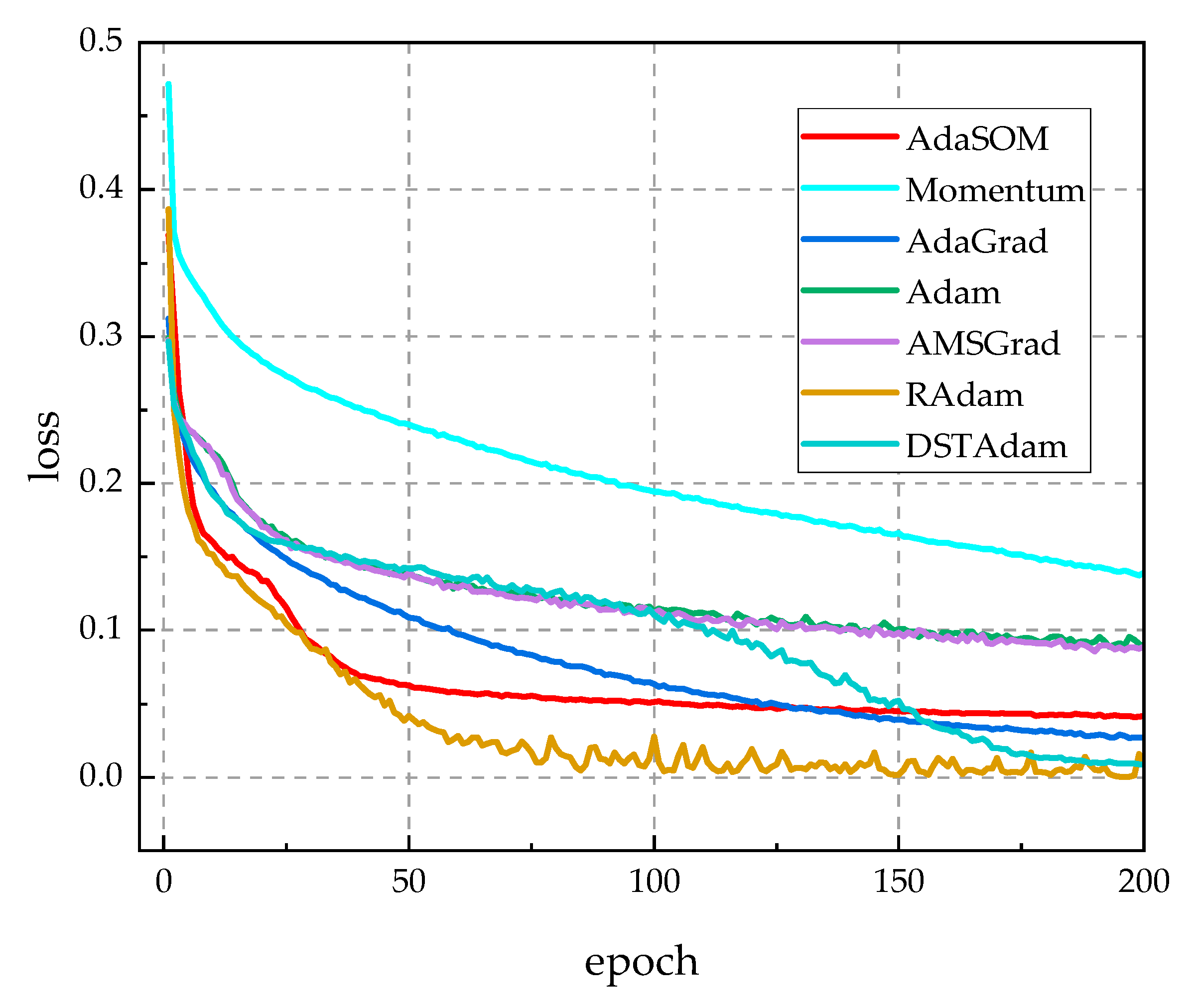
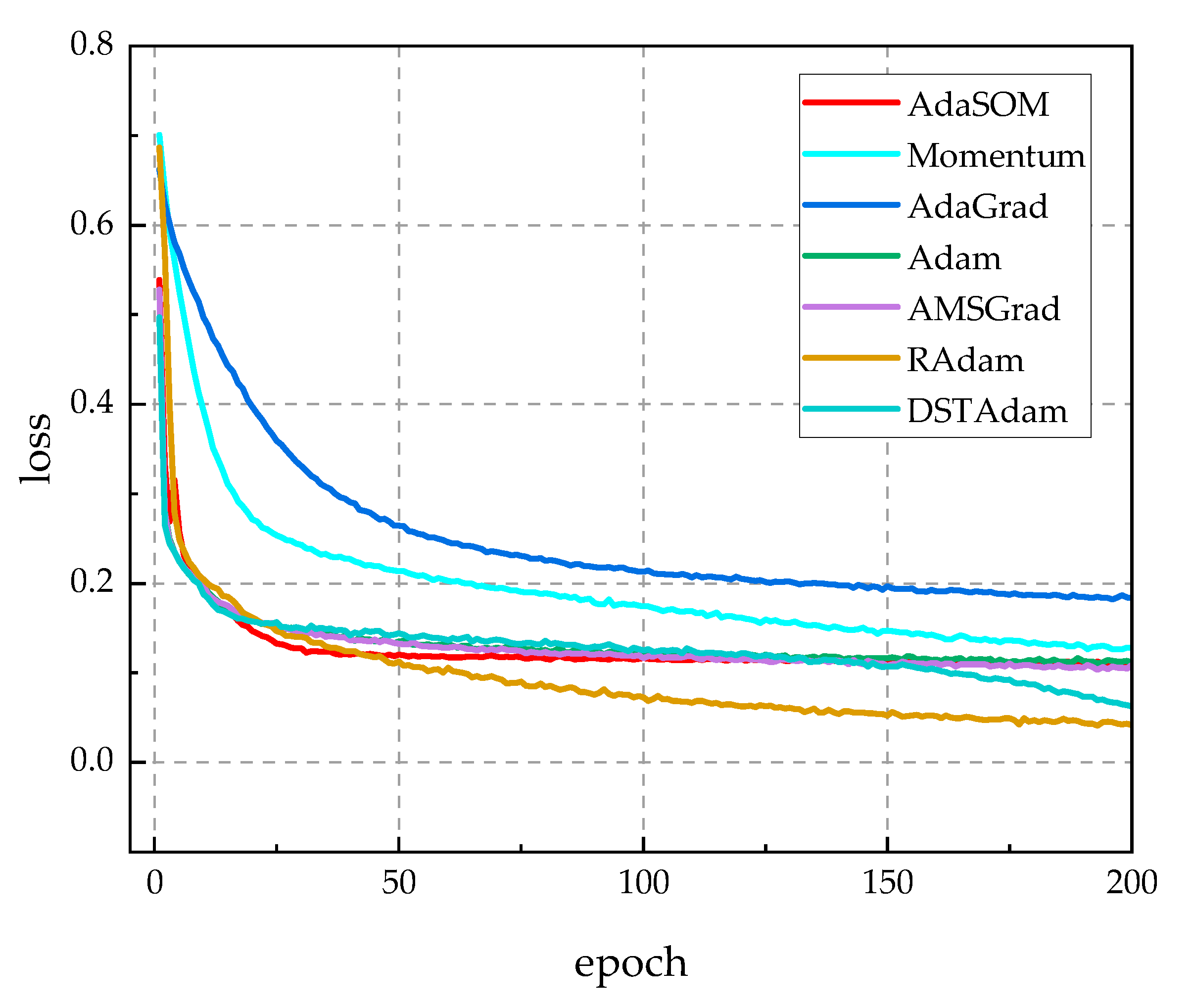
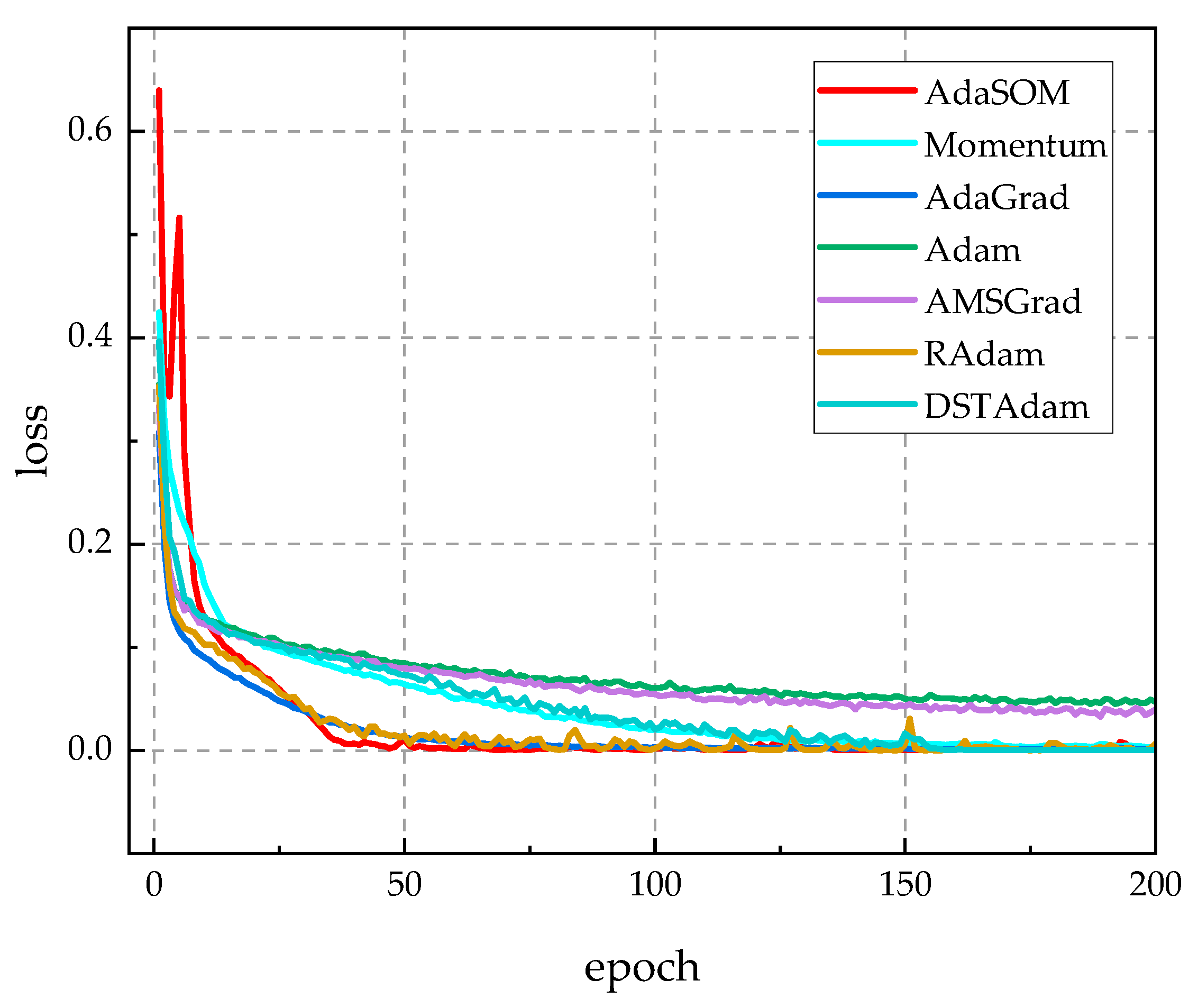
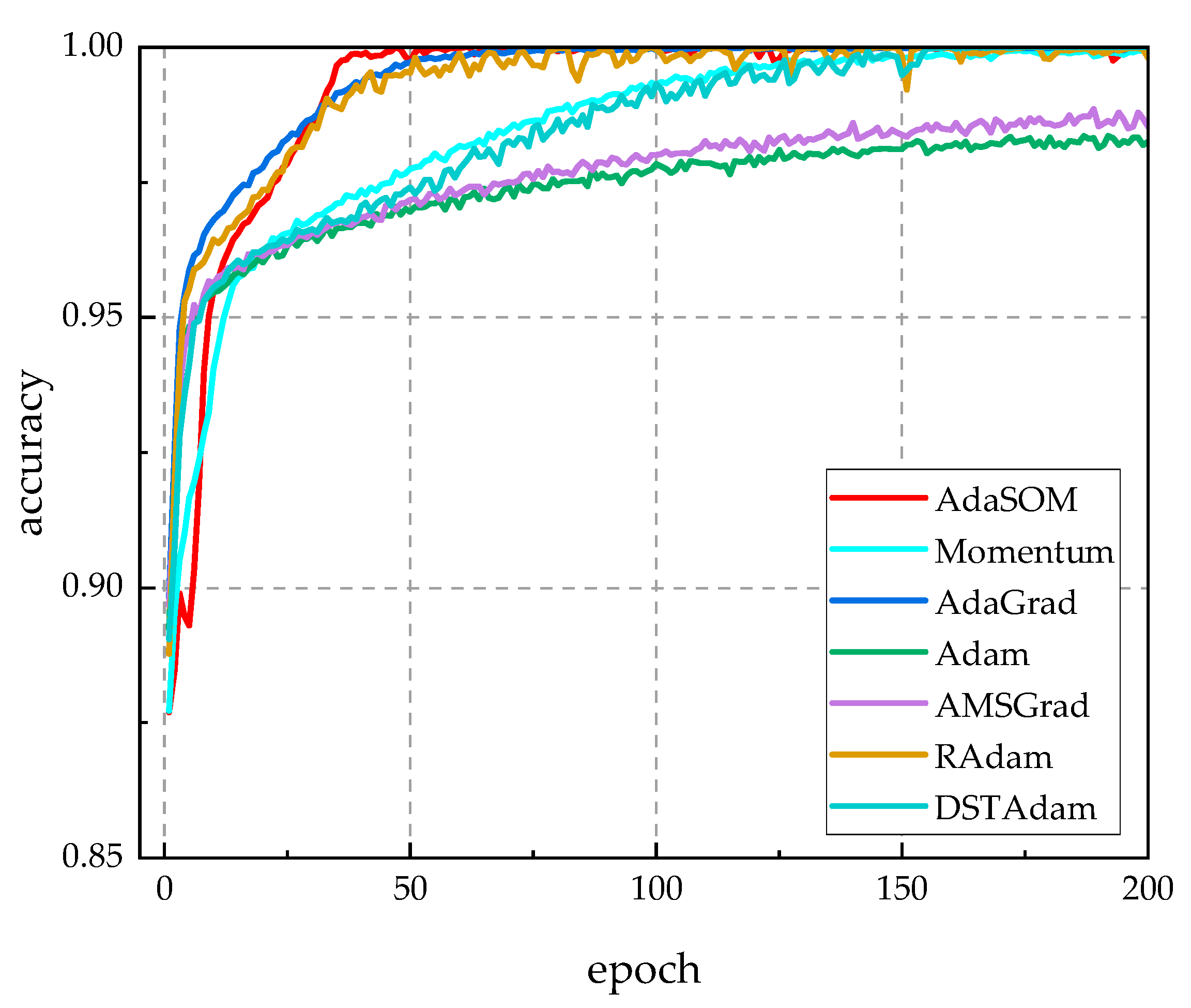
5.4.2. Comparison with Classical Training Algorithms

The AdaSOM algorithm was evaluated against several classical deep-learning training algorithms. The comparable training algorithms include momentum [23], Adam [25], AdaGrad [34], AMSGrad [35], RAdam [36], and DSTAdam [37]. Momentum represents the traditional momentum method. Adam, on the other hand, is a variant of the first-order stochastic gradient descent method that incorporates finite memory, allowing it to adjust the first-order gradient through an adaptive learning rate based on gradient direction. AdaGrad functions as a stochastic, optimized subgradient method that regulates the learning rate of the first-order gradient via a proximal function. AMSGrad enhances Adam by introducing a new learning rate aimed at improving the algorithm’s iterative convergence. RAdam modifies Adam by exploring ways to accelerate its convergence rate through the proper initialization of the learning rate. Lastly, DSTAdam implements a mechanism that gradually transitions from the Adam algorithm to stochastic gradient descent during iterations, effectively combining the strengths of both approaches.

The initial learning rate for the optimization algorithms was established at 1 × 10⁻³ [38], with the exception of momentum, which had an initial learning rate set to 1 × 10⁻¹ [23]. For the AdaSOM algorithm, the initial learning rate and momentum coefficient were configured to 2 × 10⁻⁵ and 0.9, respectively. Additionally, the weight decay rate for all the optimization algorithms was fixed at 5 × 10⁻⁴. The mini-batch size was determined to be 32.

Figure 3 describes the changing curves of the loss function values for each competitive optimization algorithm on the training set throughout the training process. From Figure 3, the following is evident: (1) in comparison to the momentum algorithm, the AdaSOM algorithm demonstrated a significantly faster decrease in loss function values, indicating that the proposed adaptive learning rate incorporating second-order gradient information effectively accelerated convergence for the momentum algorithm. (2) When compared to the DSTAdam algorithm, AdaSOM exhibited smoother convergence during iterations, whereas DSTAdam displayed pronounced jagged peaks indicative of iterative oscillations; thus, AdaSOM’s convergence stability surpassed that of DSTAdam during optimization. (3) The trends of loss function values during iterations for AdaSOM closely resembled those of Adam, AdaGrad, AMSGrad, and RAdam—all exhibiting a clear convergence trend. Therefore, Figure 3 confirms that by introducing an adaptive learning rate with second-order gradient information, the AdaSOM algorithm can significantly enhance both convergence speed and stability relative to the momentum algorithm; consequently, the improvement ideas proposed in this paper are effective and feasible.

Figure 4 reveals the accuracy curves of competing algorithms throughout the training process. From Figure 4, it is evident that the iterative accuracy trends of the AdaSOM algorithm, as well as those of AdaGrad, AMSGrad, and DSTAdam, all approached 100%, indicating that the AdaSOM algorithm successfully converged during training. In the later stages of training, however, the accuracy of AdaGrad, AMSGrad, and DSTAdam exhibited oscillations, whereas the curve for AdaSOM remained relatively smooth. Furthermore, in Figure 3 and Figure 4, the convergence behavior aligned perfectly with our theoretical analysis regarding the convergence properties of the AdaSOM algorithm presented in Section 4. Through the analysis of the results presented in

Table 4. Metric values for related algorithms on the test set.

Algorithm	Acc	P	R	F1	AUC
Momentum [23]	0.9608 ± 0.0126	0.8302 ± 0.0108	0.8641 ± 0.0112	0.8452 ± 0.0110	0.9673 ± 0.0125
AdaGrad [35]	0.9689 ± 0.0127	0.8459 ± 0.0111	0.8381 ± 0.0113	0.8381 ± 0.0112	0.9688 ± 0.0127
Adam [25]	0.9691 ± 0.0118	0.8612 ± 0.0105	0.8389 ± 0.0102	0.8469 ± 0.0103	0.9702 ± 0.0118
AMSGrad [34]	0.9682 ± 0.0105	0.8392 ± 0.0091	0.8482 ± 0.0092	0.8419 ± 0.0091	0.9706 ± 0.0105
Radam [36]	0.9703 ± 0.0101	0.8446 ± 0.0088	0.8491 ± 0.0088	0.8411 ± 0.0087	0.9685 ± 0.0100
DSTAdam [37]	0.9712 ± 0.0105	0.8437 ± 0.0091	0.8533 ± 0.0092	0.8475 ± 0.0092	0.9693 ± 0.0105
AdaSOM (Ours)	0.9768 ± 0.0173	0.8812 ± 0.0156	0.8446 ± 0.0150	0.8616 ± 0.0152	0.9742 ± 0.0173

, it becomes evident that utilizing a learning rate informed by second-order information allows for better adaptation to current momentum conditions, which enhances the training stability and enables the algorithm to identify more optimal weights to fit the training dataset effectively—ultimately leading to a higher model training accuracy rate.

Figure 5 illustrates the loss function curves of competing algorithms on the validation set throughout the training process. As observed in Figure 5, the AdaSOM algorithm exhibited the lowest loss function value among all the evaluated algorithms, indicating that its generalization capability on the validation set was significantly superior to that of comparable algorithms. Notably, during the later stages of training, the loss value for the AdaSOM algorithm gradually stabilized, suggesting an enhanced ability to maintain model stability and generalization capacity as training progresses. Therefore, Figure 4 demonstrates that the 1D-ResNet model trained by the AdaSOM algorithm possesses greater robustness and generalization ability.

To assess the model independence of the AdaSOM algorithm, we trained the AlexNet [39], VGG11 [40], and Inception [41] models on the CPCS2018 dataset, utilizing the AdaSOM. The resulting models have been designated as AlexNet-AdaSOM, VGG11-AdaSOM, and Inception-AdaSOM, respectively. Figure A1, Figure A2 and Figure A3 in Appendix A illustrate a comparison of the training loss function curves for these three models across relevant algorithms. From these figures, it is evident that the AdaSOM algorithm demonstrates strong convergence across all three models, thereby indicating its model-independent nature.

Table 4 presents the metric values of the competing algorithms evaluated on the test set. As illustrated in Table 4, the F1 score of the AdaSOM algorithm reached 0.8616, which was an improvement of 1.66% over the second-ranked DSTAdam algorithm. Furthermore, the AdaSOM algorithm demonstrated superior performance compared to other algorithms in terms of accuracy, precision, and AUC metrics. Although the accuracy rates of all training algorithms in Figure 4 were close to 100%, the model trained by AdaSOM had the highest F1 and AUC values in Table 4. This indicated that the AdaSOM algorithm possessed superior optimization capabilities, enabling it to identify more optimal weights for accurately fitting the features of the training samples; consequently, the trained model exhibited an enhanced generalization ability and achieved higher classification accuracy on the test set. The results presented in Table 4 confirm that enhancements made to the momentum algorithm within this study significantly improve classification accuracy for 12-lead ECGs, thus validating both the effectiveness and feasibility of our proposed improvements.

5.4.3. Comparison with State-of-the-Art Deep-Learning Models

The 1D-Resnet-AdaSOM model was compared with several state-of-the-art deep-learning models, with data for these baseline models sourced from their original publications. The results obtained on the CPSC2018 dataset are presented in

Table 5. Comparison of the results of related deep-learning models on the CPSC2018 dataset.

Deep Model	Acc	P	R	AUC	F1
MTNN [42]	0.966	0.852	0.808	0.977	0.827
lightX3ECG [43]	0.963	0.821	0.786	—	0.800
ED-DGCN [44]	—	0.849	0.841	—	0.843
STFAC-Net [45]	0.894	0.778	0.756	0.933	0.767
LFG-Net [46]	—	0.853	0.838	—	0.842
No. CPSC0236 [47]	0.970	—	—	0.911	0.840
Bean [48]	—	0.706	0.715	0.928	0.711
resnet_wang [48]	—	0.692	0.700	0.924	0.689
Xresnet1d101 [48]	—	0.690	0.697	0.924	0.671
JAMC [51]	0.706	—	—	0.915	0.666
SCDNN [52]	0.859	0.838	0.781	—	0.782
Inception-CL [53]	—	—	—	—	0.710
AlexNet-AdaSOM	0.963	0.811	0.813	0.969	0.811
Inception-AdaSOM	0.962	0.787	0.784	0.970	0.781
VGG11-AdaSOM	0.949	0.729	0.793	0.963	0.756
1D-ResNet34-AdaSOM	0.977	0.881	0.845	0.974	0.862

. In this table, the symbol “—” indicates that the original literature does not provide these data. The multi-task neural network (MTNN) [42] employs SE-ResNet to extract ECG features and dynamically captures both the local and global information of ECG signal feature sequences through CoT within the classification module. The lightX3ECG model [43] utilizes three independent one-dimensional convolutional neural networks (1D-CNNs) as its backbone to extract features from each of the three input ECG leads. The ED-DGCN model [44] leverages a convolutional neural network (CNN) during the encoder stage to extract feature information from ECG signals, while employing a bi-directional LSTM in the decoder stage to delineate semantic regions and generate corresponding class relations. The STFAC-Net model [45] enhances the overall performance by integrating advantages derived from CNNs, RNNs, and Transformers. The LFG-Net [46] applies the Shapley additive explanations (SHAP) methodology to select lead features that exhibit high contributions. No. CPSC0236 was the team number of a participant in the CPSC 2018 competition, where they achieved first place overall [47]. The Bean model is a multibranch network for 12-lead electrocardiogram multilabel classification based on ensemble learning and attention [48]. The resnet_wang model is a ResNet network used for time series classification [49]. The Xresnet model is a ResNet network that has been improved with over a dozen tricks [50]. The JAMC model is an autoencoder with masked contrastive learning [51]. The SCDNN model is a convolutional neural network that embeds frequency and time-domain information [52]. Inception-CL is an Inception network with domain knowledge-driven contrastive learning [53].

As illustrated in Table 5, the average F1 score of the 1D-ResNet-AdaSOM model was 0.862, demonstrating superior classification performance. The models resnet_wang, Xresnet101, and 1D-ResNet34-AdaSOM are all categorized as ResNet-type deep networks. However, the average F1 score of 1D-ResNet34-AdaSOM surpasses that of resnet_wang and Xresnet101 by 25.11% and 28.46%, respectively. Notably, despite having a lower model complexity than Xresnet101, 1D-ResNet34-AdaSOM demonstrates more robust recognition performance for 12-lead ECG signals. Models such as Bean, JAMC, SCDNN, STFAC-Net, and lightX3ECG have made significant strides in extracting deep features from 12-lead ECGs. However, their F1 scores are generally low, suggesting that while optimizing the deep features of ECG is important, the training algorithms employed by these models also play a critical role in the recognition and effective utilization of these features. The F1 score of model No. CPSC0236, which achieved first place in the CPSC2018 competition, is 0.84. Among the models presented in Table 5, those that demonstrate superior F1 scores compared to No. CPSC0236 include ED-DGCN, LFG-Net, and 1D-ResNet34-AdaSOM. The distinguishing feature of the LFG-Net model lies in its ability to identify and prioritize the lead features that significantly contribute to classification, representing a form of feature enhancement technology. The ED-DGCN model leverages the larger-scale PTB-XL dataset for auxiliary training, thereby enhancing its capability to recognize the characteristics of 12-lead ECG signals through an increased data scale. Both models, Inception-AdaSOM and Inception-CL, are categorized as Inception-type deep networks. However, the F1 score of the former surpasses that of the latter by 10%. This observation further underscores the significant influence that training algorithms exert on deep-learning models for ECG classification. The models AlexNet-AdaSOM, Inception-AdaSOM, VGG11-AdaSOM, and 1D-ResNet34-AdaSOM were trained utilizing the AdaSOM. While their architectures remained unchanged, their F1 scores ranked among the highest compared to other models evaluated. This further underscores the effectiveness of AdaSOM in enhancing the classification accuracy of deep-learning networks for 12-lead ECG analysis. Based on the analysis of the data in Table 5, the competing models employed more intricate feature extraction methods to enhance the ECG classification accuracy. However, in contrast to competing models, we retained the original 1D-ResNet architecture, resulting in a structurally simpler and computationally lighter framework; notably, this unmodified architecture achieved high ECG classification accuracy via an enhanced adaptive training algorithm. The analysis of the results in Table 5 validates our hypothesis that optimizing the learning rate within the training algorithm can effectively enhance ECG classification accuracy for the 1D-ResNet model.

6. Conclusions

When classifying 12-lead ECGs using deep-learning models, conventional research approaches primarily focus on enhancing accuracy through the adoption of novel deep feature extraction methods to capture more comprehensive local and global features of ECG signals. In contrast to the traditional literature, the innovation of this paper lies in improving the classification accuracy of 1D-ResNet-34 for 12-lead ECGs by optimizing the training algorithm’s learning rate. Specifically, we perform a Taylor expansion on the iterative formula governing the weights of the 1D-ResNet model to derive a learning rate that incorporates second-order gradient information. Given that accurately calculating the Hessian matrix for obtaining second-order gradient information poses significant challenges, we propose an approach to approximate the second-order gradient information by utilizing the historical first-order gradient. Accordingly, an adaptive learning rate is derived, incorporating second-order gradient information. Furthermore, to mitigate issues related to excessively large or small learning rates during iterations—which could adversely impact both stability and accuracy—we implement a truncation mechanism for the learning rate. Finally, we validate the classification performance of our proposed model, termed 1D-ResNet-AdaSOM, on the CPSC2018 dataset. The experimental results indicate that our model’s loss function converges effectively during training with reduced oscillations compared to competing algorithms; additionally, it achieves a commendable average F1 score of 0.862 on the test set. These results demonstrate that the proposed model has superior classification performance and generalization capabilities when compared with state-of-the-art competing deep-learning models. In summary, 1D-ResNet-AdaSOM is lightweight in structure and robust in 12-lead ECG classification performance.

Although the proposed method significantly enhances the classification accuracy of 1D-ResNet for 12-lead ECGs, certain limitations persist. (1) The training algorithm presented in this paper struggles to effectively address the accuracy of minority categories. For instance, as illustrated in Figure 2, the minority category PAC is frequently misclassified as Normal at a relatively high proportion. (2) It remains to be investigated whether combining the AdaSOM algorithm with state-of-the-art deep features can further enhance ECG classification accuracy within deep-learning models. (3) The mathematical formulas employed in the AdaSOM algorithm are modality-independent and theoretically applicable to any modality. However, the effectiveness of its application in other modalities, such as images and signals, requires further investigation. These issues will be subject to ongoing exploration in future research endeavors.

References

1. Zhang, Q.-x.; Liu, Z.-j.; Liu, X.-h.; Zhao, X.-h.; Li, X.-c. The Correlation between Epicardial Adipose Tissue Thickness Measured by Echocardiography and P-Wave Dispersion and Atrial Fibrillation. Rev. Cardiovasc. Med. 2024, 25, 287. [Google Scholar] [CrossRef] [PubMed]
2. Nechita, L.C.; Nechita, A.; Voipan, A.E.; Voipan, D.; Debita, M.; Fulga, A.; Fulga, I.; Musat, C.L. AI-Enhanced ECG Applications in Cardiology: Comprehensive Insights from the Current Literature with a Focus on COVID-19 and Multiple Cardiovascular Conditions. Diagnostics 2024, 14, 1839. [Google Scholar] [CrossRef] [PubMed]
3. Kalmady, S.V.; Salimi, A.; Sun, W.; Sepehrvand, N.; Nademi, Y.; Bainey, K.; Ezekowitz, J.; Hindle, A.; McAlister, F.; Greiner, R. Development and validation of machine learning algorithms based on electrocardiograms for cardiovascular diagnoses at the population level. npj Digit. Med. 2024, 7, 133. [Google Scholar] [CrossRef] [PubMed]
4. Ameen, A.; Fattoh, I.E.; Abd El-Hafeez, T.; Ahmed, K. Advances in ECG and PCG-based cardiovascular disease classification: A review of deep learning and machine learning methods. J. Big Data 2024, 11, 159. [Google Scholar] [CrossRef]
5. Padmavathi, S.; Ramanujam, E. Naïve Bayes classifier for ECG abnormalities using multivariate maximal time series motif. Procedia Comput. Sci. 2015, 47, 222–228. [Google Scholar] [CrossRef]
6. Hamidi, A.A.; Robertson, B.; Ilow, J. A new approach for ECG artifact detection using fine-KNN classification and wavelet scattering features in vital health applications. Procedia Comput. Sci. 2023, 224, 60–67. [Google Scholar] [CrossRef]
7. Hamza, S.; Ayed, Y.B. Svm for human identification using the ECG signal. Procedia Comput. Sci. 2020, 176, 430–439. [Google Scholar] [CrossRef]
8. Ambrish, G.; Ganesh, B.; Ganesh, A.; Srinivas, C.; Mensinkal, K. Logistic regression technique for prediction of cardiovascular disease. Glob. Transit. Proc. 2022, 3, 127–130. [Google Scholar]
9. Vimal, C.; Sathish, B. Random forest classifier based ECG arrhythmia classification. Int. J. Healthc. Inf. Syst. Inform. (IJHISI) 2010, 5, 1–10. [Google Scholar] [CrossRef]
10. Xu, Y.; Zhang, S.; Cao, Z.; Chen, Q.; Xiao, W. Extreme Learning Machine for Heartbeat Classification with Hybrid Time-Domain and Wavelet Time-Frequency Features. J. Healthc. Eng. 2021, 2021, 6674695. [Google Scholar] [CrossRef]
11. El-Khafif, S.H.; El-Brawany, M.A. Artificial Neural Network-Based Automated ECG Signal Classifier. Int. Sch. Res. Not. 2013, 2013, 261917. [Google Scholar] [CrossRef]
12. Liu, L.-R.; Huang, M.-Y.; Huang, S.-T.; Kung, L.-C.; Lee, C.-h.; Yao, W.-T.; Tsai, M.-F.; Hsu, C.-H.; Chu, Y.-C.; Hung, F.-H. An Arrhythmia classification approach via deep learning using single-lead ECG without QRS wave detection. Heliyon 2024, 10, e27200. [Google Scholar] [CrossRef] [PubMed]
13. Darmawahyuni, A.; Nurmaini, S.; Tutuko, B.; Rachmatullah, M.N.; Firdaus, F.; Sapitri, A.I.; Islami, A.; Marcelino, J.; Isdwanta, R.; Perwira, M.I. An improved electrocardiogram arrhythmia classification performance with feature optimization. BMC Med. Inform. Decis. Mak. 2024, 24, 412. [Google Scholar] [CrossRef]
14. Toulni, Y.; Nsiri, B.; Drissi, T.B. ECG signal classification using DWT, MFCC and SVM classifier. Trait. Du Signal 2023, 40, 335. [Google Scholar] [CrossRef]
15. Guo, Y.; Liu, Y.; Oerlemans, A.; Lao, S.; Wu, S.; Lew, M.S. Deep learning for visual understanding: A review. Neurocomputing 2016, 187, 27–48. [Google Scholar] [CrossRef]
16. Liu, X.; Wang, H.; Li, Z.; Qin, L. Deep learning in ECG diagnosis: A review. Knowl.-Based Syst. 2021, 227, 107187. [Google Scholar] [CrossRef]
17. Ahmed, A.A.; Ali, W.; Abdullah, T.A.; Malebary, S.J. Classifying cardiac arrhythmia from ECG signal using 1D CNN deep learning model. Mathematics 2023, 11, 562. [Google Scholar] [CrossRef]
18. Hou, B.; Yang, J.; Wang, P.; Yan, R. LSTM-based auto-encoder model for ECG arrhythmias classification. IEEE Trans. Instrum. Meas. 2019, 69, 1232–1240. [Google Scholar] [CrossRef]
19. Jahmunah, V.; Ng, E.Y.; Tan, R.-S.; Oh, S.L.; Acharya, U.R. Explainable detection of myocardial infarction using deep learning models with Grad-CAM technique on ECG signals. Comput. Biol. Med. 2022, 146, 105550. [Google Scholar] [CrossRef]
20. Strodthoff, N.; Wagner, P.; Schaeffter, T.; Samek, W. Deep learning for ECG analysis: Benchmarks and insights from PTB-XL. IEEE J. Biomed. Health Inform. 2020, 25, 1519–1528. [Google Scholar] [CrossRef]
21. Hempel, P.; Ribeiro, A.H.; Vollmer, M.; Bender, T.; Dörr, M.; Krefting, D.; Spicher, N. Explainable AI associates ECG aging effects with increased cardiovascular risk in a longitudinal population study. npj Digit. Med. 2025, 8, 25. [Google Scholar] [CrossRef] [PubMed]
22. He, K.; Zhang, X.; Ren, S.; Sun, J. Deep residual learning for image recognition. In Proceedings of the IEEE Conference on Computer Vision and Pattern Recognition, Las Vegas, NV, USA, 26 June–1 July 2016; pp. 770–778. [Google Scholar]
23. Sutskever, I.; Martens, J.; Dahl, G.; Hinton, G. On the importance of initialization and momentum in deep learning. In Proceedings of the 30th International Conference on Machine Learning, Atlanta, GA, USA, 16–21 June 2013; Sanjoy, D., David, M., Eds.; PMLR (Proceedings of Machine Learning Research): New York, NY, USA, 2013; Volume 28, pp. 1139–1147. [Google Scholar]
24. Gitman, I.; Lang, H.; Zhang, P.; Xiao, L. Understanding the role of momentum in stochastic gradient methods. In Proceedings of the Advances in Neural Information Processing Systems, Vancouver, BC, Canada, 8–14 December 2019; Volume 32. [Google Scholar]
25. Kingma, D.P.; Ba, J. Adam: A method for stochastic optimization. arXiv 2014, arXiv:1412.6980. [Google Scholar]
26. Burdakov, O.; Dai, Y.; Huang, N. Stabilized barzilai-borwein method. J. Comput. Math. 2019, 37, 916–936. [Google Scholar] [CrossRef]
27. Castera, C.; Bolte, J.; Févotte, C.; Pauwels, E. Second-order step-size tuning of SGD for non-convex optimization. Neural Process. Lett. 2022, 54, 1727–1752. [Google Scholar] [CrossRef]
28. Liu, F.; Liu, C.; Zhao, L.; Zhang, X.; Wu, X.; Xu, X.; Liu, Y.; Ma, C.; Wei, S.; He, Z. An open access database for evaluating the algorithms of electrocardiogram rhythm and morphology abnormality detection. J. Med. Imaging Health Inform. 2018, 8, 1368–1373. [Google Scholar] [CrossRef]
29. Zhang, D.; Yang, S.; Yuan, X.; Zhang, P. Interpretable deep learning for automatic diagnosis of 12-lead electrocardiogram. iScience 2021, 24, 102373. [Google Scholar] [CrossRef]
30. Ribeiro, A.H.; Ribeiro, M.H.; Paixão, G.M.; Oliveira, D.M.; Gomes, P.R.; Canazart, J.A.; Ferreira, M.P.; Andersson, C.R.; Macfarlane, P.W.; Meira, W., Jr. Automatic diagnosis of the 12-lead ECG using a deep neural network. Nat. Commun. 2020, 11, 1760. [Google Scholar] [CrossRef]
31. Jothiaruna, N. SSDMNV2-FPN: A cardiac disorder classification from 12 lead ECG images using deep neural network. Microprocess. Microsyst. 2022, 93, 104627. [Google Scholar]
32. Yao, Q.; Wang, R.; Fan, X.; Liu, J.; Li, Y. Multi-class arrhythmia detection from 12-lead varied-length ECG using attention-based time-incremental convolutional neural network. Inf. Fusion 2020, 53, 174–182. [Google Scholar] [CrossRef]
33. Baloglu, U.B.; Talo, M.; Yildirim, O.; San Tan, R.; Acharya, U.R. Classification of myocardial infarction with multi-lead ECG signals and deep CNN. Pattern Recognit. Lett. 2019, 122, 23–30. [Google Scholar] [CrossRef]
34. Duchi, J.; Hazan, E.; Singer, Y. Adaptive subgradient methods for online learning and stochastic optimization. J. Mach. Learn. Res. 2011, 12, 2121–2159. [Google Scholar]
35. Reddi, S.J.; Kale, S.; Kumar, S. On the convergence of adam and beyond. arXiv 2019, arXiv:1904.09237. [Google Scholar]
36. Liu, L.; Jiang, H.; He, P.; Chen, W.; Liu, X.; Gao, J.; Han, J. On the variance of the adaptive learning rate and beyond. arXiv 2019, arXiv:1908.03265. [Google Scholar]
37. Zeng, K.; Liu, J.; Jiang, Z.; Xu, D. A decreasing scaling transition scheme from Adam to SGD. Adv. Theory Simul. 2022, 5, 2100599. [Google Scholar] [CrossRef]
38. Qiu, L.; Cai, W.; Zhang, M.; Zhu, W.; Wang, L. Two-stage ECG signal denoising based on deep convolutional network. Physiol. Meas. 2021, 42, 115002. [Google Scholar] [CrossRef]
39. Krizhevsky, A.; Sutskever, I.; Hinton, G.E. ImageNet classification with deep convolutional neural networks. Commun. ACM 2017, 60, 84–90. [Google Scholar] [CrossRef]
40. Simonyan, K.; Zisserman, A. Very deep convolutional networks for large-scale image recognition. arXiv 2014, arXiv:1409.1556. [Google Scholar]
41. Szegedy, C.; Liu, W.; Jia, Y.; Sermanet, P.; Reed, S.; Anguelov, D.; Erhan, D.; Vanhoucke, V.; Rabinovich, A. Going Deeper with Convolutions. In Proceedings of the IEEE Conference on Computer Vision and Pattern Recognition (CVPR), Boston, MA, USA, 7–12 June 2015; pp. 1–9. [Google Scholar]
42. Geng, Q.; Liu, H.; Gao, T.; Liu, R.; Chen, C.; Zhu, Q.; Shu, M. An ECG Classification Method Based on Multi-Task Learning and CoT Attention Mechanism. Healthcare 2023, 11, 1000. [Google Scholar] [CrossRef]
43. Le, K.H.; Pham, H.H.; Nguyen, T.B.; Nguyen, T.A.; Thanh, T.N.; Do, C.D. Lightx3ecg: A lightweight and explainable deep learning system for 3-lead electrocardiogram classification. Biomed. Signal Process. Control 2023, 85, 104963. [Google Scholar] [CrossRef]
44. Cheng, Y.; Zhu, W.; Li, D.; Wang, L. Multi-label classification of arrhythmia using dynamic graph convolutional network based on encoder-decoder framework. Biomed. Signal Process. Control 2024, 95, 106348. [Google Scholar] [CrossRef]
45. Yang, Z.; Jin, A.; Li, Y.; Yu, X.; Xu, X.; Wang, J.; Li, Q.; Guo, X.; Liu, Y. A coordinated adaptive multiscale enhanced spatio-temporal fusion network for multi-lead electrocardiogram arrhythmia detection. Sci. Rep. 2024, 14, 20828. [Google Scholar] [CrossRef] [PubMed]
46. Cheng, Y.; Li, D.; Wang, D.; Chen, Y.; Wang, L. Multi-label arrhythmia classification using 12-lead ECG based on lead feature guide network. Eng. Appl. Artif. Intell. 2024, 129, 107599. [Google Scholar] [CrossRef]
47. Chen, T.-M.; Huang, C.-H.; Shih, E.S.; Hu, Y.-F.; Hwang, M.-J. Detection and classification of cardiac arrhythmias by a challenge-best deep learning neural network model. iScience 2020, 23, 100886. [Google Scholar] [CrossRef]
48. Wang, X.; Wang, N.; Liu, D.; Wu, J.; Lu, P. Bean: A Multibranch Network for 12 Leads Electrocardiogram Multilabel Classification Based on Ensemble Learning and Attention. IEEE Trans. Instrum. Meas. 2025, 74, 4005313. [Google Scholar] [CrossRef]
49. Wang, Z.; Yan, W.; Oates, T. Time Series Classification from Scratch with Deep Neural Networks: A Strong Baseline. In Proceedings of the 2017 International Joint Conference on Neural Networks (IJCNN), Anchorage, AK, USA, 14–19 May 2017; pp. 1578–1585. [Google Scholar]
50. He, T.; Zhang, Z.; Zhang, H.; Zhang, Z.; Xie, J.; Li, M. Bag of Tricks for Image Classification with Convolutional Neural Networks. In Proceedings of the IEEE/CVF Conference on Computer Vision and Pattern Recognition (CVPR), Long Beach, CA, USA, 16–20 June 2019; pp. 558–567. [Google Scholar]
51. Ge, Y.; Zhang, H.; Shi, J.; Luo, D.; Chang, S.; He, J.; Huang, Q.; Wang, H. JAMC: A jigsaw-based autoencoder with masked contrastive learning for cardiovascular disease diagnosis. Knowl.-Based Syst. 2025, 311, 113090. [Google Scholar] [CrossRef]
52. Liu, C.; Cheng, S.; Ding, W.; Arcucci, R. Spectral cross-domain neural network with soft-adaptive threshold spectral enhancement. IEEE Trans. Neural Netw. Learn. Syst. 2023, 36, 692–703. [Google Scholar] [CrossRef]
53. Zhou, S.; Huang, X.; Liu, N.; Zhang, W.; Zhang, Y.-T.; Chung, F.-L. Open-world electrocardiogram classification via domain knowledge-driven contrastive learning. Neural Netw. 2024, 179, 106551. [Google Scholar] [CrossRef]
Figure 1. The architecture of the 1D-ResNet-34 model for ECG classification.
Electronics 14 01941 g001
Figure 2. The confusion matrix of 1D-ResNet-AdaSOM on the test set.
Electronics 14 01941 g002
Figure 3. The loss function curves of related algorithms throughout the training process.
Electronics 14 01941 g003
Figure 4. The accuracy rate curves of related algorithms during the training process.
Electronics 14 01941 g004
Figure 5. The loss function curves of related algorithms on the validation set.
Electronics 14 01941 g005