
From Single to Deep Learning and Hybrid Ensemble Models for Recognition of Dog Motion States †


Abstract
1. Introduction
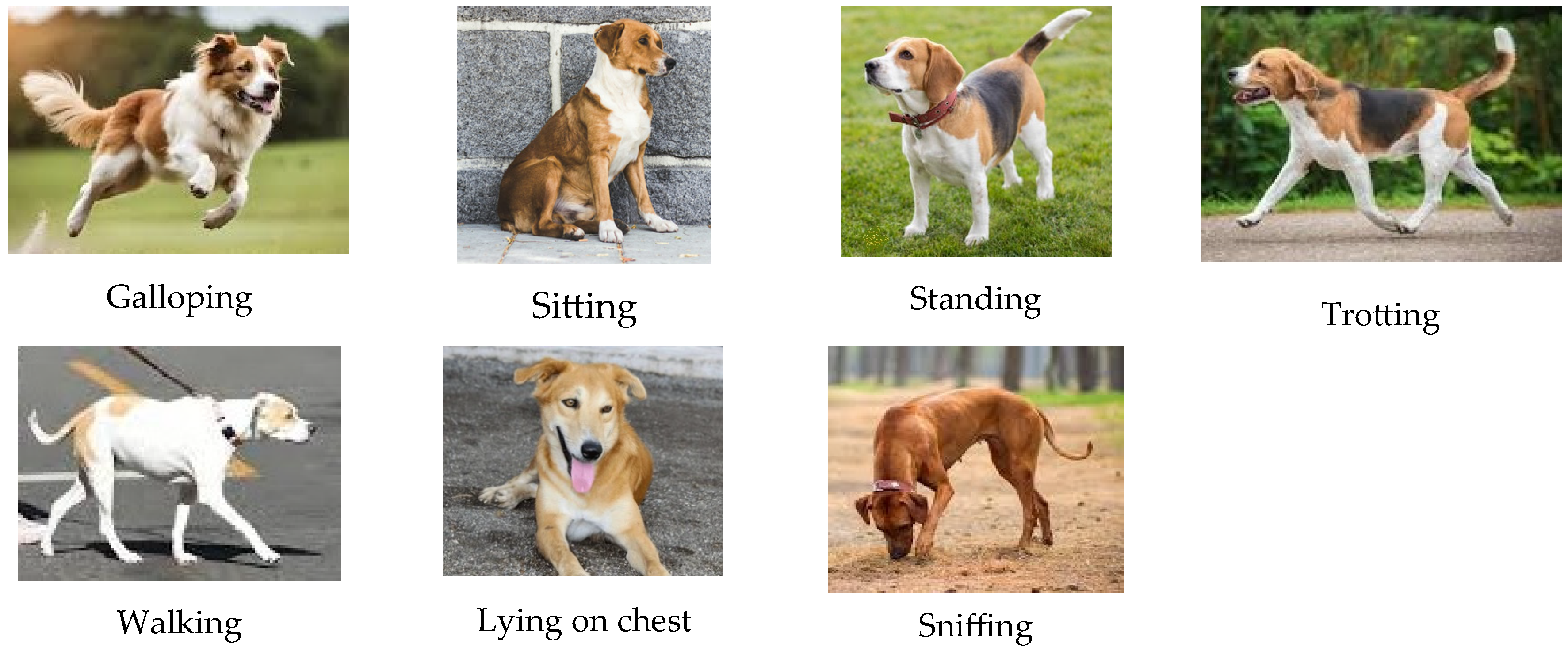
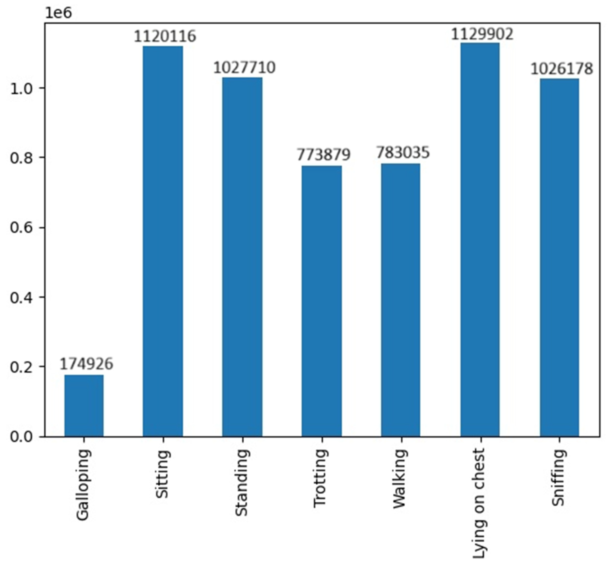
- An extended dataset that concerns seven dog motion states, rather than five as in [13], is used.
- A new stacking model, called the Compound Stacking Model (CSM), is configured and used.
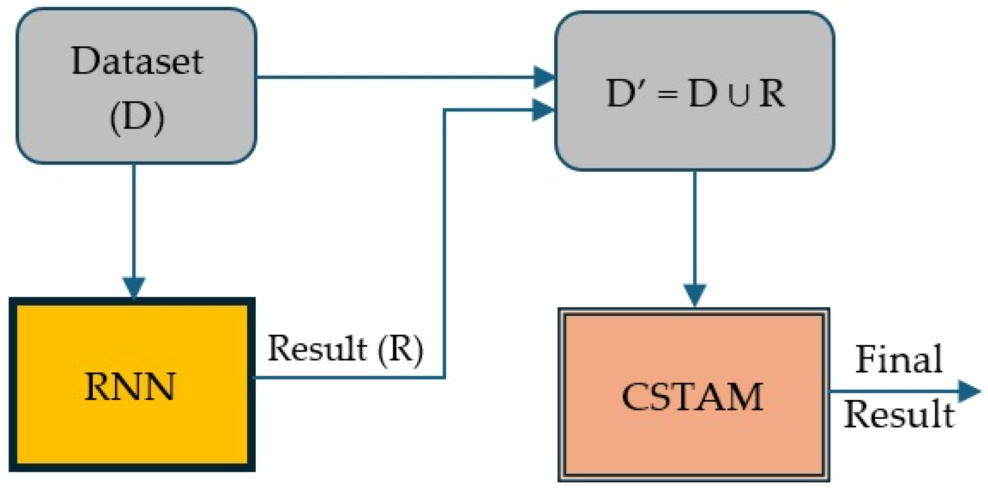
- A new hybrid cascading model (HCM), combining RNN and CSM models, is introduced and used. HCM produces the best accuracy result that overcomes almost all SOTA systems.
- Comparison with old and new state-of-the-art models is presented.
- Useful conclusions about the scalability of the used models and the recognition difficulty level of dog motion states are drawn.
2. Related Work
3. Materials and Methods
3.1. Datasets and Preprocessing
3.2. Experimental Methodology
- Application of the same classification models as those configured and tested for datset-5 ms in [13] to dataset-7 ms, so that we can see their behavior at an extended dataset.
- Analysis of the new results and comparison with the old ones.
- In case of non-satisfactory results, design and train new compound models.
- Random Forest (RF).
- Bagging model (BM) with DT as base classifier.
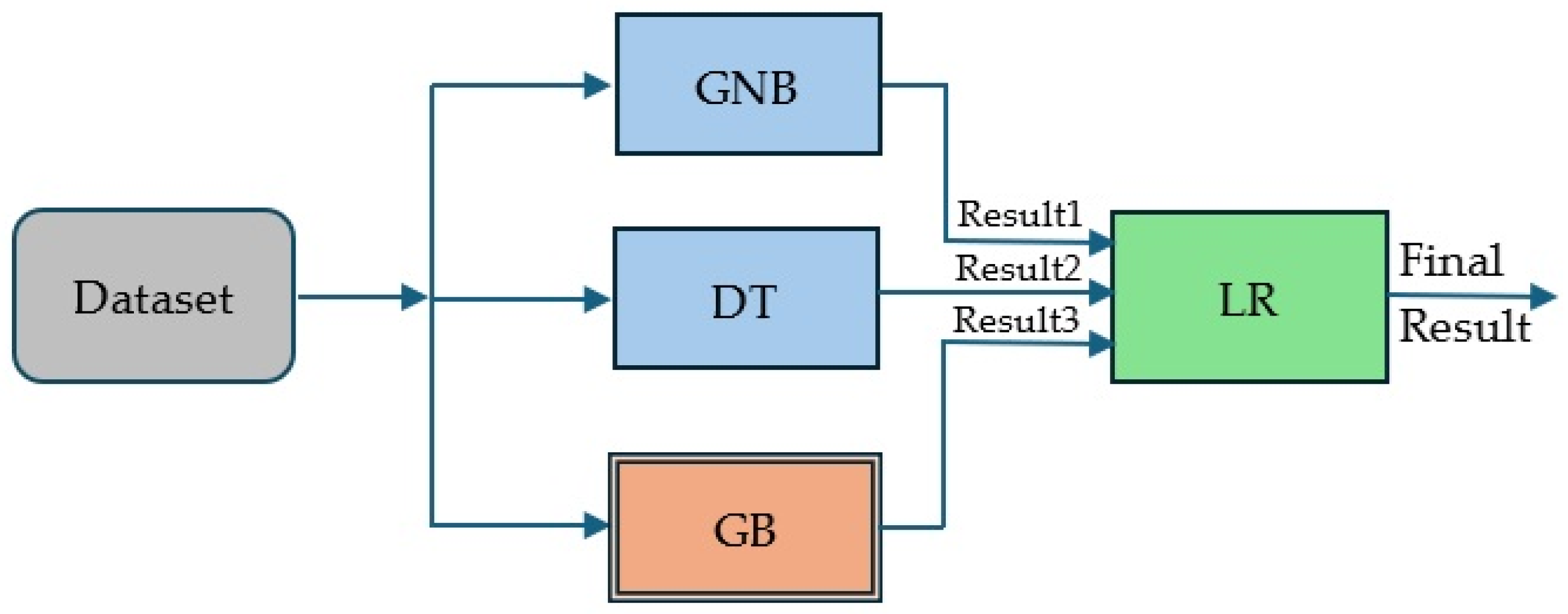
- Stacking model (SM) with k-NN and DT as base models, and LR as meta-classifier.
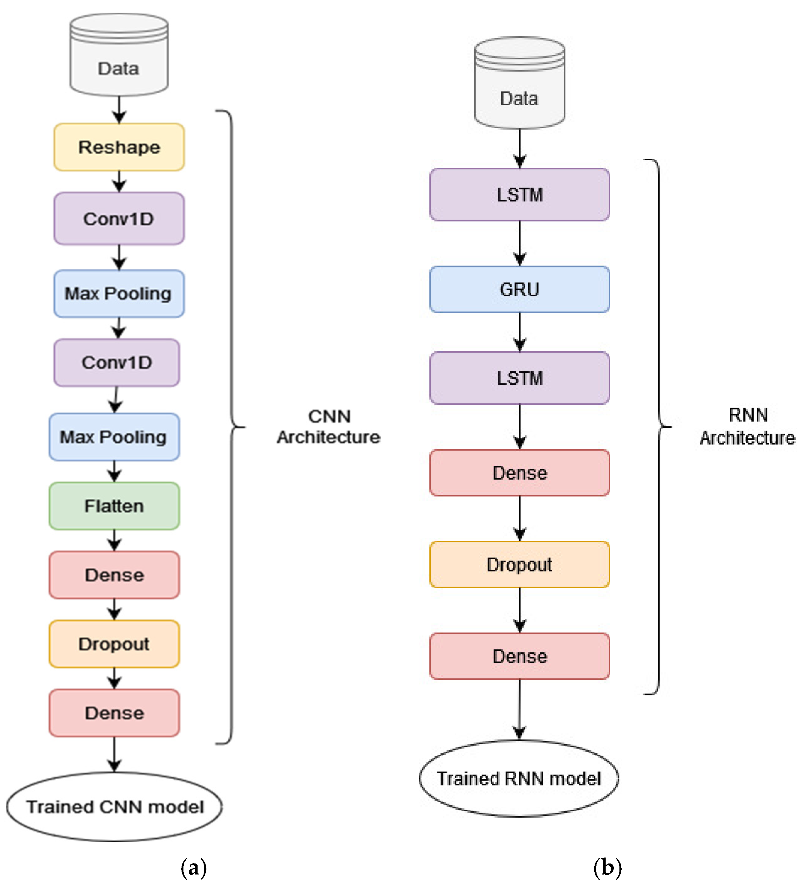
- Convolutional Neural Network (CNN)
- Recurrent Neural Network (RNN)
- Use an ensemble model as an extra base model in SM, thus creating a compound stacking model (CSM). As a compound stacking model, we define the one that includes one (or more) stacking model(s) as base classifier(s) or meta-classifier. We chose Gradient Boosting (GB) as an extra base model, because this model had the best results from all ensemble models in [13].
- Combine the best ensemble model with the best deep learning model in a cascading mode, thus creating a hybrid cascading model (HCM). As a hybrid cascading model, we define a cascading model that mixes (conventional) ML models with DL models. This gave us the best result.
3.3. Implementation Tools and Metrics
4. Experimental Results
5. Comparisons and Discussion
6. Conclusions
Author Contributions
Funding
Data Availability Statement
Conflicts of Interest
Appendix A


References
- Hardin, A.; Schlupp, I. Using machine learning and DeepLabCut in animal behavior. Acta Ethologica 2022, 25, 125–133. [Google Scholar] [CrossRef]
- Mao, A.; Huang, E.; Wang, X.; Liu, K. Deep learning-based animal activity recognition with wearable sensors: Overview, challenges, and future directions. Comput. Electron. Agric. 2023, 211, 108043. [Google Scholar] [CrossRef]
- Kamat, Y.; Nasnodkar, S. Advances in technologies and methods for behavior, emotion, and health monitoring in pets. Appl. Res. Artif. Intell. Claud Comput. 2018, 1, 38–57. [Google Scholar]
- Väätäjä, H.; Majaranta, P.; Isokoski, P.; Gizatdinova, Y.; Kujala, M.V.; Somppi, S.; Vehkaoja, A.; Vainio, O.; Juhlin, O.; Ruohonen, M.; et al. Happy dogs and happy owners: Using dog activity monitoring technology in everyday life. In Proceedings of the 5th International Conference on Animal-Computer Interaction, Atlanta, GA, USA, 4–6 December 2018; pp. 1–12. [Google Scholar] [CrossRef]
- Rast, W.; Kimmig, S.E.; Giese, L.; Berger, A. Machine learning goes wild: Using data from captive individuals to infer wildlife behaviors. PLoS ONE 2020, 15, e0227317. [Google Scholar] [CrossRef] [PubMed]
- Borah, B.; Saikia, R.; Das, P. Animal Motion Tracking in Forest: Using Machine Vision Technology. Int. J. Sci. Res. Eng. Manag. (IJSREM) 2022, 6, 1–8. [Google Scholar] [CrossRef]
- Kasnesis, P.; Doulgerakis, V.; Uzunidis, D.; Kogias, D.G.; Funcia, S.I.; Gonz’alez, M.B.; Giannousis, C.; Patrikakis, C.Z. Deep learning empowered wearable-based behavior recognition for search and rescue dogs. Sensors 2022, 22, 993. [Google Scholar] [CrossRef] [PubMed]
- Ferdinandy, B.; Gerencser, L.; Corrieri, L.; Perez, P.; Ujvary, D.; Csizmadia, G.; Miklosi, A. Challenges of machine learning model validation using correlated behaviour data: Evaluation of cross-validation strategies and accuracy measures. PLoS ONE 2020, 15, e0236092. [Google Scholar] [CrossRef] [PubMed]
- Hussain, A.; Sikandar, A.; Abdullah Hee-Cheol, K. Activity Detection for the Wellbeing of Dogs Using Wearable Sensors Based on Deep Learning. IEEE Access 2022, 10, 53153–53163. [Google Scholar] [CrossRef]
- Hussain, A.; Begum, K.; Armand, T.P.T.; Mozumder, A.I.; Ali, S.; Kim, H.C.; Joo, M.-I. Long Short-Term Memory (LSTM)-Based Dog Activity Detection Using Accelerometer and Gyroscope. Appl. Sci. 2022, 12, 9427. [Google Scholar] [CrossRef]
- Hatzilygeroudis, I.; Prentzas, J. AI Approaches for the Prognosis of the Survival (or Not) of Patients with Bone Metastases. In Proceedings of the IEEE 33rd International Conference on Tools with Artificial Intelligence (ICTAI), Washington, DC, USA, 1–3 November 2021; pp. 1353–1357. [Google Scholar] [CrossRef]
- Troussas, C.; Krouska, A.; Virvou, M. Evaluation of ensemble-based sentiment classifiers for Twitter data. In Proceedings of the 7th International Conference on Information, Intelligence, Systems & Applications (IISA), Chalkidiki, Greece, 13–15 July 2016; pp. 1–6. [Google Scholar] [CrossRef]
- Davoulos, G.; Lalakou, I.; Hatzilygeroudis, I. Recognition of Dog Motion States: Ensemble vs Deep Learning Models. In Proceedings of the 15th International Conference on Information, Intelligence, Systems & Applications (IISA), Chania Crete, Greece, 17–19 July 2024; pp. 1–8. [Google Scholar] [CrossRef]
- Aich, S.; Chakraborty, S.; Sim, J.-S.; Jang, D.-J.; Kim, H.-C. The Design of an Automated System for the Analysis of the Activity and Emotional Patterns of Dogs with Wearable Sensors Using Machine Learning. Appl. Sci. 2019, 9, 4938. [Google Scholar] [CrossRef]
- Chambers, R.D.; Yoder, N.C.; Carson, A.B.; Junge, C.; Allen, D.E.; Prescott, L.M.; Bradley, S.; Wymore, G.; Lloyd, K.; Lyle, S. Deep Learning Classification of Canine Behavior Using a Single Collar-Mounted Accelerometer: Real-World Validation. Animals 2021, 11, 1549. [Google Scholar] [CrossRef] [PubMed]
- Kumpulainen, P.; Cardo, A.V.; Somppi, S.; Tornqvist, H.; Vaataja, H.; Majaranta, P.; Gizatdinova, Y.; Antink, C.H.; Surakka, V.; Kujala, M.V.; et al. Dog behaviour classification with movement sensors placed on the harness and the collar. Appl. Anim. Behav. Sci. 2021, 241, 105393. [Google Scholar] [CrossRef]
- Vehkaoja, A.; Somppi, S.; Törnqvist, H.; Cardó, A.V.; Kumpulainen, P.; Väätäjä, H.; Majaranta, P.; Surakka, V.; Kujala, M.V.; Vainio, O. Description of Movement Sensor Dataset for Dog Behavior Classification. Data Brief 2022, 40, 107822. [Google Scholar] [CrossRef] [PubMed]
- Muminov, A.; Mukhiddinov, M.; Cho, J. Enhanced Classification of Dog Activities with Quaternion-Based Fusion Approach on High-Dimensional Raw Data from Wearable Sensors. Sensors 2022, 22, 9471. [Google Scholar] [CrossRef] [PubMed]
- Amano, R.; Ma, J. Recognition and Change Point Detection of Dogs’ Activities of Daily Living Using Wearable Devices. In Proceedings of the 2021 IEEE Intl Conf on Dependable, Autonomic and Secure Computing, Intl Conf on Pervasive Intelligence and Computing, Intl Conf on Cloud and Big Data Computing, Intl Conf on Cyber Science and Technology Congress, Virtual, 25–28 October 2021; pp. 693–699. [Google Scholar] [CrossRef]
- Kim, J.; Moon, N. Dog Behavior Recognition Based on Multimodal Data from a Camera and Wearable Device. Appl. Sci. 2022, 12, 3199. [Google Scholar] [CrossRef]
- Eerdekens, A.; Callaert, A.; Deruyck, M.; Martens, L.; Joseph, W. Dog’s Behaviour Classification Based on Wearable Sensor Accelerometer Data. In Proceedings of the 5th Conference on Cloud and Internet of Things (CIoT-22), Marrakech, Morocco, 28–30 March 2022; pp. 226–231. [Google Scholar]
- Kim, H.; Moon, N. TN-GAN-Based Pet Behavior Prediction through Multiple-Dimension Time-Series Augmentation. Sensors 2023, 23, 4157. [Google Scholar] [CrossRef] [PubMed]
- Marcato, M.; Tedesco, S.; O’Mahony, C.; O’Flynn, B.; Galvin, P. Machine learning based canine posture estimation using inertial data. PLoS ONE 2023, 18, e0286311. [Google Scholar] [CrossRef] [PubMed]
- Or, B. Transformer Based Dog Behavior Classification with Motion Sensors. IEEE Sens. J. 2024, 24, 33816–33825. [Google Scholar] [CrossRef]
- Chatzilygeroudis, K.; Hatzilygeroudis, I.; Perikos, I. Machine Learning Basics. In Intelligent Computing for Interactive System Design: Statistics, Digital Signal Processing, and Machine Learning in Practice; ACM: New York, NY, USA, 2021; pp. 143–193. [Google Scholar] [CrossRef]
- Garcıa-Pedrajas, N.; Ortiz-Boyer, D.; del Castillo-Gomariz, R.; Hervas-Martınez, C. Cascade Ensembles. In Computational Intelligence and Bioinspired Systems. IWANN 2005; Cabestany, J., Prieto, A., Sandoval, D.F., Eds.; Lecture Notes in Computer Science; Springer: Berlin/Heidelberg, Germany, 2005; Volume 3512. [Google Scholar] [CrossRef]
- De Zarzà, I.; de Curtò, J.; Hernández-Orallo, E.; Calafate, C.T. Cascading and Ensemble Techniques in Deep Learning. Electronics 2023, 12, 3354. [Google Scholar] [CrossRef]


| Motion State | Description |
|---|---|
| Galloping | A 3- or 4-beat gait where the dog lifts and puts down both front and rear extremities in a coordinated manner, in 1-2-3-beat gait (canter) or in 1-2-3-4 beat gait (gallop). All four extremities are simultaneously in the air at some point in every stride. Galloping occurred only during the Playing task. |
| Sitting | The dog has four extremities and rump on the ground. The dog can change the balance point from central to hip or vice versa. |
| Standing | The dog has the four extremities on the ground, without the dog’s torso touching the ground. |
| Trotting | A 2-beat gait where the dog lifts and puts down extremities in diagonal pairs at a speed faster than walking. |
| Walking | A 4-beat gait where the dog moves extremities at slow speed, legs are moved one by one in the order: left hind leg, left front leg, right hind leg, and right front leg. The dog moves straight forward or at a maximum angle of 45 degrees. |
| Lying on chest | The dog’s torso is touching the ground, and its hips are at the same level as its shoulders. The dog can change balance point without using its limbs. |
| Sniffing | The dog has its head below its back line and moves its muzzle close to the ground. The dog walks, stands, or performs another slow movement, but its chest and bottom do not touch the ground. Taking food from the ground and eating it can be included (eating was not coded separately). |
| Column | Description |
|---|---|
| Dog ID | Number of dog ID |
| Test Num | Number of the test {1, 2} |
| t_sec | Time from the start of the test (in sec) |
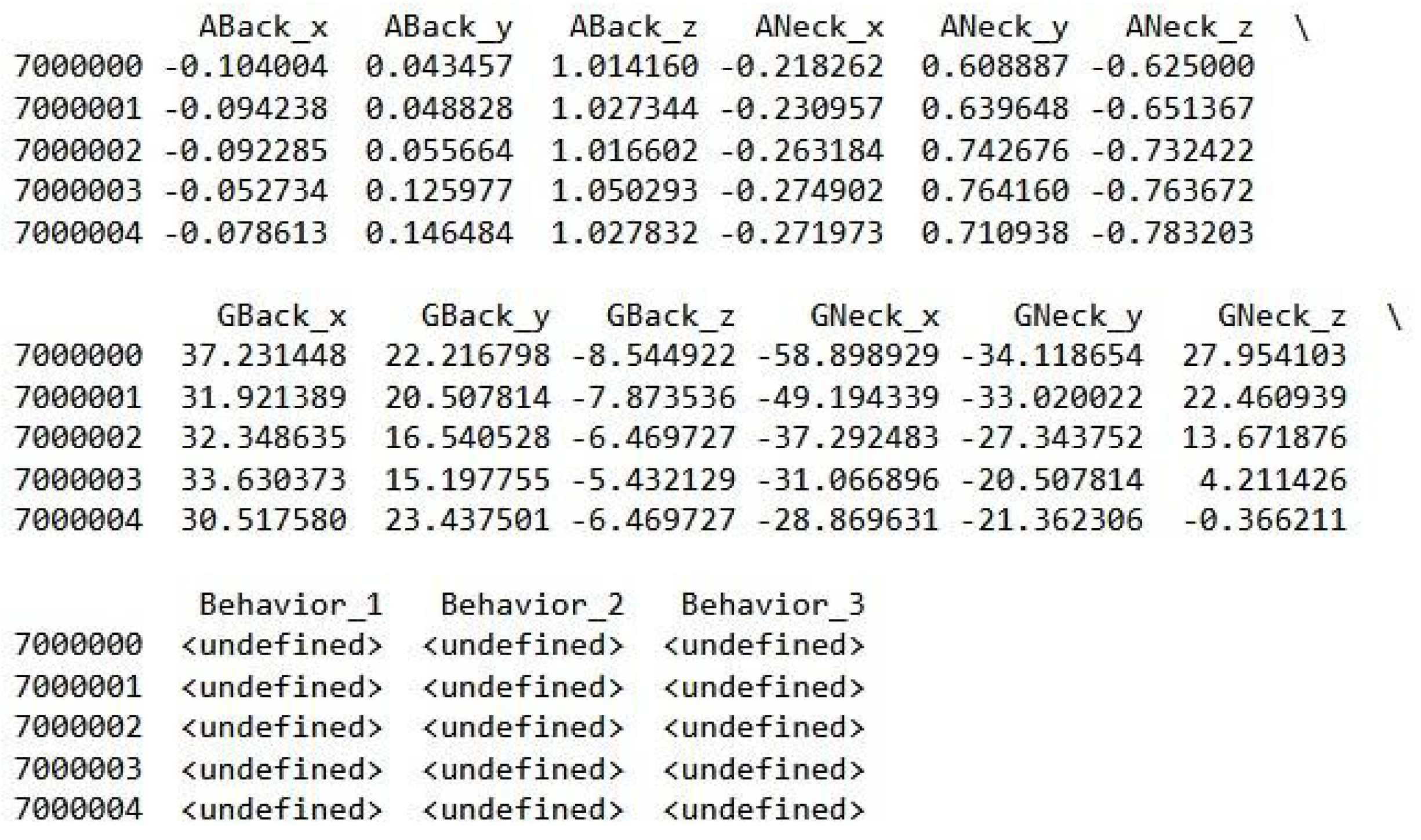
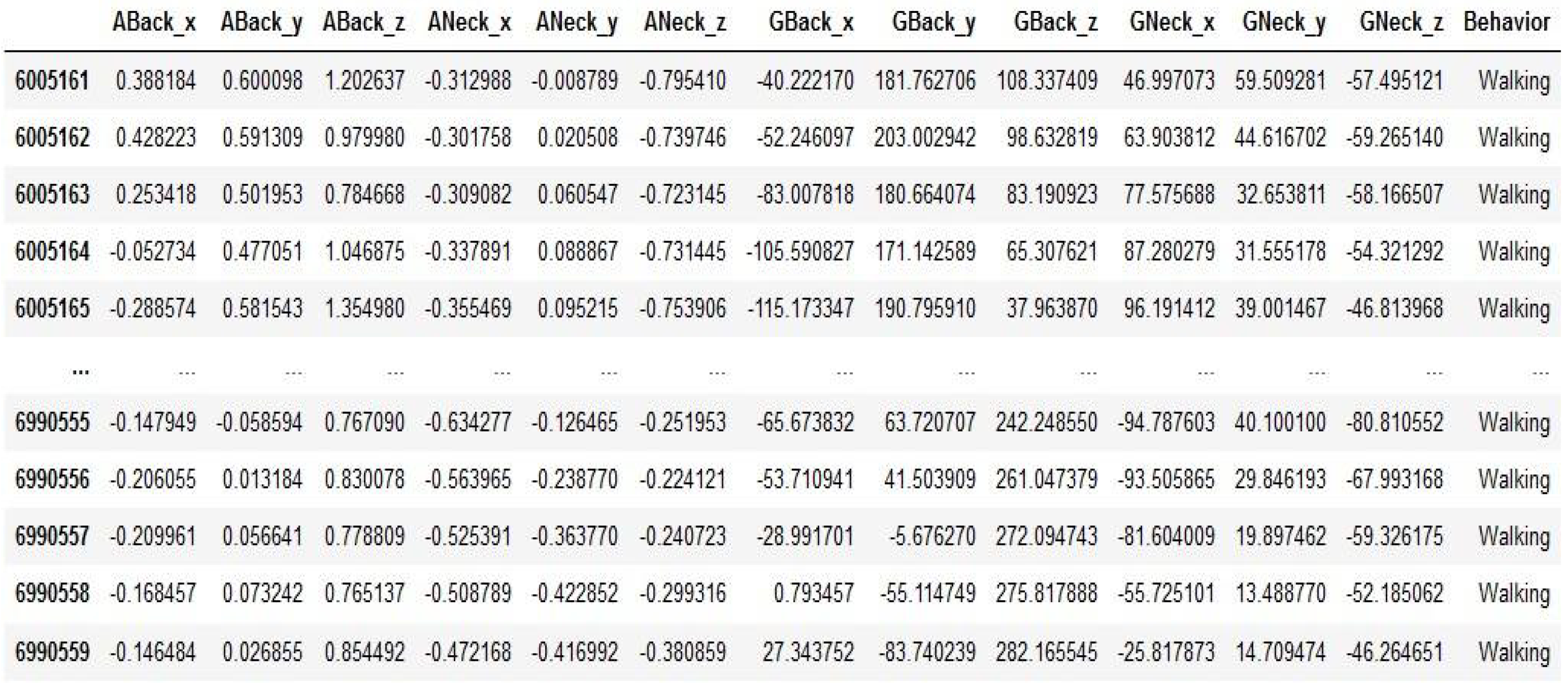
| ABack_x | Accelerometer measurement from the sensor in the back, x-axis |
| ABack_y | Accelerometer measurement from the sensor in the back, y-axis |
| ABack_z | Accelerometer measurement from the sensor in the back, z-axis |
| ANeck_x | Accelerometer measurement from the sensor in the neck, x-axis |
| ANeck_y | Accelerometer measurement from the sensor in the neck, y-axis |
| ANeck_z | Accelerometer measurement from the sensor in the neck, z-axis |
| GBack_x | Gyroscope measurement from the sensor in the back, x-axis |
| GBack_y | Gyroscope measurement from the sensor in the back, y-axis |
| GBack_z | Gyroscope measurement from the sensor in the back, z-axis |
| GNeck_x | Gyroscope measurement from the sensor in the neck, x-axis |
| GNeck_y | Gyroscope measurement from the sensor in the neck, y-axis |
| GNeck_z | Gyroscope measurement from the sensor in the neck, z-axis |
| task | The task given at the time, <undefined> when no task is being performed |
| behavior_1 | Annotated behavior 1, maximum of three simultaneous annotations at the same time |
| behavior_2 | Annotated behavior 2, maximum of three simultaneous annotations at the same time |
| behavior_3 | Annotated behavior 3, maximum of three simultaneous annotations at the same time |
| PointEvent | Short events annotated separately (Bark, for example) |
| Model | Accuracy | Precision | Recall | F1-Score | ||||
|---|---|---|---|---|---|---|---|---|
| 5 ms | 7 ms | 5 ms | 7 ms | 5 ms | 7 ms | 5 ms | 7 ms | |
| GNB | 0.88 | 0.74 | 0.88 | 0.74 | 0.88 | 0.74 | 0.88 | 0.73 |
| Decision Tree | 0.84 | 0.75 | 0.83 | 0.75 | 0.84 | 0.75 | 0.83 | 0.75 |
| k-NN | 0.78 | 0.65 | 0.78 | 0.65 | 0.78 | 0.65 | 0.78 | 0.65 |
| Random Forest | 0.90 | 0.81 | 0.90 | 0.81 | 0.90 | 0.81 | 0.90 | 0.81 |
| Bagging Model | 0.85 | 0.69 | 0.85 | 0.71 | 0.85 | 0.69 | 0.85 | 0.68 |
| Stacking Model | 0.90 | 0.81 | 0.90 | 0.81 | 0.90 | 0.81 | 0.90 | 0.81 |
| CNN | 0.93 | 0.89 | 0.93 | 0.89 | 0.93 | 0.89 | 0.93 | 0.89 |
| RNN | 0.95 | 0.93 | 0.95 | 0.93 | 0.95 | 0.93 | 0.95 | 0.93 |
| CSM | 0.91 | 0.91 | 0.91 | 0.91 | ||||
| HCM | 0.97 | 0.97 | 0.97 | 0.97 | ||||
| Model | 1st Best Feature | 2nd Best Feature | 1st Worst Feature | 2nd Worst Feature | ||||
|---|---|---|---|---|---|---|---|---|
| 5 ms | 7 ms | 5 ms | 7 ms | 5 ms | 7 ms | 5 ms | 7 ms | |
| GNB | Sitting | Sniffing | Standing | Sitting | Galloping | Standing | Walking | Lying on chest |
| Decision Tree | Sitting | Sniffing | Standing | Sitting | Galloping | Galloping | Walking | Lying on chest |
| k-NN | Trotting | Galloping | Sitting | Trotting | Standing | Standing | Galloping | Walking |
| Random Forest | Sitting | Sniffing | Standing | Sitting | Galloping | Standing | Walking | Lying on chest |
| Bagging Model | Sitting | Sniffing | Standing | Sitting | Galloping | Walking | Walking | Galloping |
| Stacking Model | Sitting | Sniffing | Trotting | Sitting | Galloping | Standing | Walking | Lying on chest |
| CNN | Sitting | Sniffing | Standing | Sitting | Galloping | Galloping | Walking | Standing |
| RNN | Sitting | Sitting | Standing | Sniffing | Galloping | Galloping | Walking | Standing |
| CSM | Sniffing | Sitting | Galloping | Standing | ||||
| HCM | Sitting | Sniffing | Galloping | Walking | ||||
| Work | Dataset | States | Approach | Acc (%) |
|---|---|---|---|---|
| Aich et al. [14]-2019 | Own | 7 | Deep MLP (6 layers) | 96.58 |
| Amano & Ma [19]-2021 | Own | 5 | CNN (2Conv, 2MaxP, 2Dropout, 1Flatten, 3FC) | 92.6 |
| Kumpulainen et al. [16]-2021 | Mendeley (part of) | 7 (Incl. Galloping) | SVM | 91.4 |
| Muminov et al. [18]-2022 | Own | 6 | GNB | 88.0 |
| Hussain et al. [9]-2022 | Own | 10 | CNN (5Conv, 2Dropout, 1Flatten, 3FC) | 96.85 |
| Hussain et al. [10]-2022 | Own | 10 | LSTM (6LSTM, 3Dropout, 3FC) | 94.25 |
| Eerdekens et al. [21]-2022 | Own | 9 (incl. Sprinting) | CNN (2Conv, 1MaxP, 1Flatten, 1FC) | 96.9 (10 Hz) |
| Marcato et al. [23]-2023 | Own | 5 | RF Cascade | 90 (F1) |
| Or [24]-2024 | Mendeley (part of) | 7 (incl. Galloping) | Encoder-FFN-GAP | 98.5–94.6 (F1) |
| Ours1 [13]-2024 | Kaggle (part of) | 5 (incl. Galloping) | RNN (2LSTM, 1GRU, 1Dropout, 2FC) | 94.7 (100 Hz) |
| Ours2 (HCM)-2025 | Kaggle (extended part of) | 7 (incl. Galloping) | RNN-CSM Cascading | 96.82 (100 Hz) |
Disclaimer/Publisher’s Note: The statements, opinions and data contained in all publications are solely those of the individual author(s) and contributor(s) and not of MDPI and/or the editor(s). MDPI and/or the editor(s) disclaim responsibility for any injury to people or property resulting from any ideas, methods, instructions or products referred to in the content. |
© 2025 by the authors. Licensee MDPI, Basel, Switzerland. This article is an open access article distributed under the terms and conditions of the Creative Commons Attribution (CC BY) license (https://creativecommons.org/licenses/by/4.0/).
Share and Cite
Davoulos, G.; Lalakou, I.; Hatzilygeroudis, I. From Single to Deep Learning and Hybrid Ensemble Models for Recognition of Dog Motion States. Electronics 2025, 14, 1924. https://doi.org/10.3390/electronics14101924
Davoulos G, Lalakou I, Hatzilygeroudis I. From Single to Deep Learning and Hybrid Ensemble Models for Recognition of Dog Motion States. Electronics. 2025; 14(10):1924. https://doi.org/10.3390/electronics14101924
Chicago/Turabian StyleDavoulos, George, Iro Lalakou, and Ioannis Hatzilygeroudis. 2025. "From Single to Deep Learning and Hybrid Ensemble Models for Recognition of Dog Motion States" Electronics 14, no. 10: 1924. https://doi.org/10.3390/electronics14101924
APA StyleDavoulos, G., Lalakou, I., & Hatzilygeroudis, I. (2025). From Single to Deep Learning and Hybrid Ensemble Models for Recognition of Dog Motion States. Electronics, 14(10), 1924. https://doi.org/10.3390/electronics14101924