Coupled Sub-Feedback Hyperchaotic Dynamical System and Its Application in Image Encryption

Abstract

Images serve as significant conduits of information and are extensively utilized in several facets of life. As chaotic encryption evolves, current chaotic key generators have grown increasingly prevalent and susceptible to compromise. We present an advanced chaos architecture that integrates numerous nonlinear functions and incorporates common chaotic maps as perturbation factors. The produced two-dimensional QWT chaotic map exhibits a more stable chaotic state and a broader chaotic range in comparison to existing maps. Simultaneously, we developed a novel roulette scrambling technique that shifts the conventional in-plane scrambling to cross-plane scrambling. Upon evaluation, the encrypted image demonstrates commendable performance regarding information entropy, correlation, and other parameters, while its encryption algorithm exhibits robust security.

1. Introduction

The Internet and communication technology are advancing at a rapid pace, and images are gradually superseding text as the primary medium for information transmission. The security and timeliness of information transmission are increasingly being prioritized, particularly in the current era of big data. Images possess the attributes of high redundancy, a large data capacity, and a strong correlation between adjacent pixels, as they differ from conventional text information [1]. Consequently, traditional encryption methods, including Advanced Encryption Standard, Data Encryption Standard, and Elliptic Curve Cryptography (ECC), are not well-suited for images [2,3]. A significant number of researchers have gravitated toward the field of image encryption algorithms due to the fact that conventional one-dimensional data encryption methods are not entirely pertinent to image encryption [4]. In this field, chaos is of paramount importance. In 1963, Edward Lorenz introduced the concept of chaotic systems while researching meteorological systems. In 1994, Claude Shannon [5] employed it for encryption due to its intricate attributes, including extreme sensitivity, unpredictability, and non-periodicity. The specific requirements of image encryption can be satisfied by the pseudo-random sequences (PRSs) that are derived from chaotic systems. This also established the groundwork for numerous chaotic encryption technologies that followed.

As a result, the discipline of cryptography has identified the issue of sustaining a chaotic system in its state of chaos and creating pseudo-random sequences as a critical research area. Aihara et al. [6] proposed a chaos model in 1990 that effectively resolved the issue of the network being captured in a locally optimal solution by combining the Hopfield network with nonlinear dynamics. Nevertheless, low-dimensional chaotic mapping continues to have deficiencies, including a restricted period window, a brief chaos period, and insufficient nonlinear dynamic characteristics. Multidimensional hyperchaotic systems have garnered an increasing amount of research interest as a solution to the issues mentioned above. Hyperchaos is indicative of the presence of more than two Lyapunov exponents in a chaotic system [7]. A variety of strategies have been proposed to circumvent the limitations of one-dimensional chaotic maps. The cascade method was employed by Zhou et al. [8] to construct a novel chaotic system by connecting two simple one-dimensional chaotic maps. The innovation is the utilization of the logistic formula as the key to regulating the iterative relationship between the triangular map and the tent map. Based on the experiment’s information entropy, it was determined that the chaotic sequences that were constructed have an influence on one another. In addition to this method of toggling chaotic effects by range, there are additional methods, such as coupling and combination [9], that can be used to create new chaotic systems. In order to progressively construct chaotic systems, trigonometric functions are frequently employed to generate numerical oscillations.

In recent years, various construction methods have been employed to propose novel hyperchaos systems [10,11,12], and the performance of many of these far surpasses that of traditional chaotic mapping. Nevertheless, these chaotic systems still possess substantial flaws, such as the initial value being insufficiently sensitive, which leads to an insufficient fluctuation of the generated sequence, thereby significantly increasing the likelihood of being breached. Images cannot be effectively utilized in the context of image encryption due to the fact that they frequently contain private and sensitive information. Nevertheless, a method of constructing chaotic systems using optimized test functions has been proposed [13], and technology is constantly evolving. In comparison to the methods that were previously employed, this function demonstrates a greater number of leaping characteristics in space. Additionally, the three-dimensional graph that results from its oscillation is more intricate. Consequently, the chaotic mapping that this function generates is more appropriate for encryption applications.

Teng et al. [14] integrated the sine function into the infinite folding mapping framework using the cross-mapping method and created a hyperchaotic system with two positive Lyapunov exponents. A study using numbers shows that for a certain range of parameters, the system has stable hyperchaotic dynamics, with a maximum Lyapunov exponent that is 42% higher than that of a normal one-dimensional system. Sun et al. [15] used a symmetric structural design method to connect the sine function with the infinite folding map in both directions. This made it possible to cover more hyperchaotic states in the parameter space. The phase diagram trajectory has interesting fractal properties between $\mu =3.6$ and 4.0, and the Kolmogorov entropy is found to be $1.83\pm 0.05$. A group of people from Hua University [16] created a new two-dimensional system by expanding the phase space dimension and combining logistic mapping and sine mapping into a single architecture. The model has a sample entropy value of about 2.0 when the parameter $\alpha$ is between 0.8 and 1.2. Its Lyapunov exponent spectrum changes by $\pm 0.15$ over long iterations, which suggests that the system has periodic windows that come and go. Ref. [10] were able to dynamically improve discrete mapping by using the oscillation mechanism of trigonometric functions. In the range of parameters $\tau$ between 1.5 and 2.5, the system they made kept the hyperchaotic state going for 37% longer than the baseline model. The combined Chebyshev-sine-cosine mapping introduced by Qin et al. [17] demonstrates distinct stability properties. The double maximum Lyapunov exponents are stable at ${\lambda }_1\approx 0.68$ and ${\lambda }_2\approx 0.52$. The NIST test pass rate attains 98.6%, confirming its viability in information encryption applications. A new study by Wang et al. [18] created a multi-parameter domain hyperchaotic system by using logistic mapping and sinusoidal coupling together in a way that works well. It has three positive Lyapunov exponents at the same time in the range $\mu =[3.2,4.0]$, and the Hausdorff dimension of its phase space trajectory reaches $1.92\pm 0.03$. The cubic-infinite folding hybrid model suggested by Wang et al. [19] demonstrates unique entropy features. The sample entropy is consistently measured at $1.6\pm 0.1$, while the permutation entropy approaches the theoretical maximum of 1.0. However, the Lyapunov exponent spectrum exhibits a bistable distribution (${\lambda }_1\approx 0.85$, ${\lambda }_2\approx 0.72$), indicating distinctive dynamic equilibrium properties. A thorough comparison reveals a distinct trade-off between system complexity and practical performance: trigonometric function coupling systems (e.g., [14,15,17]) have better entropy but are more sensitive to parameters. On the other hand, hybrid architecture systems (e.g., [16,18,19]) are very good at keeping parameters stable, but they make computations 23% more difficult on average. The primary objective of hyperchaos is to enhance the efficiency of mitigating chaotic qualities.

Diffusion and scrambling are the primary principles of image encryption algorithms. If further subdivided, they can be categorized as bit level, pixel level, and block level based on the encryption method. These methods involve encryption operations on a single bit of a single pixel value, a single pixel value, and a local block, respectively. Wang, X. et al. [20] developed a bit-level image encryption method that is highly complex; however, there is potential for enhancement in the encryption time. Gao, Q. [21] presented a 3D coordinate scrambling algorithm that is combined with a pixel-level image encryption algorithm to accomplish the effective encryption of image information. Cao, P. et al. [22] proposed a sliding window technology that is based on block encryption. This technology has the potential to increase the complexity of scrambling and strengthen the connection between blocks. The field of image encryption algorithms has recently made significant progress as a result of the integration of multiple disciplines. For instance, it has been improved by incorporating DNA encryption [23,24], quantum encryption [25,26], and other technologies, or by combining it with deep-learning-based image recognition technology [27] to achieve the double-layer encryption of privacy areas [28]. This has significantly expanded the diversity of encryption technology. These algorithms are not extensively used due to their high complexity, high time complexity, and technical barriers, despite their positive performance in certain new performance evaluations.

We included chaotic interference elements in a coupled self-feedback control, developed a novel chaos generation architecture, and integrated two nonlinear functions, the W/Wavy function and the Quartic function, into it. Subsequently, we employed logistic mapping as interference variables to create a novel chaotic dynamics model. At the same time, we found ways to make the current image encryption algorithm even better. We took the standard roulette permutation algorithm and expanded it from pixels to bits, then combined it with the double-layer diffusion algorithm to create a new image encryption algorithm. This new algorithm was then compared to the newest image encryption technologies. The principal findings of this study are as follows:

(1)

We have developed a novel method for chaos enhancement control. The W/Wavy function and Quartic function serve as the foundation for chaotic functions in coupled self-feedback systems. A novel chaotic system is developed utilizing logistic mapping as the perturbation factor. We evaluate and contrast the Lyapunov index, sample entropy, and permutation entropy with the established two-dimensional hyperchaos. The system presented in this work exhibits superior chaotic features, indicating the efficacy of the architecture.

(2)

A new three-dimensional roulette coordinate scrambling algorithm has been created. It adds the cross-plane bit level to the traditional plane-based roulette scrambling algorithm, which makes it easier to break the correlation between unit pixels and makes image encryption work better.

(3)

A double-layer diffusion algorithm is introduced. By combining the three-dimensional roulette coordinate scrambling method with the double-layer cross-channel method, the encryption algorithm works better while still being safe. We evaluate the encryption algorithm against the current one to determine its viability.

The remainder of this paper is structured as follows. The chaotic system is constructed in Section 2 using the optimized test function. An analysis of the system’s dynamics is conducted in Section 3. The color image encryption scheme’s scrambling and diffusion algorithms are explained in detail in Section 4. Multiple indicators are employed to verify the encryption scheme’s security in Section 5. Finally, Section 6 provides a summary of the work that has been completed and an outlook on the future.

2. Related Work

We have developed and introduced a novel two-dimensional coupled chaotic system, 2D-WQT, in this chapter. Based on this, we conducted an analysis of its dynamic characteristics in chaos, evaluated its various performance indicators, and obtained a chaotic sequence that can be employed in our image encryption section.

2.1. Primal Function 1

Courrieu introduced the W/Wavy function in 1997 [29]. This function is frequently employed as a benchmark in optimization problems due to its inherent concavity and convexity, as well as the existence of numerous local optimal solutions. Its precise mathematical expression is as follows:

$$f\left(x\right)=1-{\displaystyle \frac{1}{D}}\sum _{i=1}^D\cos \left(k{x}_i\right)\times e^{{\displaystyle \frac{-{x_i}^2}{2}}},$$

(1)

The specific style of the W/Wavy function in two-dimensional space is illustrated in Figure 1, which incorporates the cosine term $\mathrm{c}\mathrm{o}\mathrm{s}\left(k{x}_i\right)$ and the exponential term $e^{{\displaystyle \frac{-{x_i}^2}{2}}}$. Its lowest point is located at $x=y=0$, and it exhibits numerous peaks and valleys, which are represented by numerous local maxima and local minima. The W/Wavy function can exhibit erratic behavior through iteration, as demonstrated by subsequent experiments. This results in the generation of a time series that is a critical element of image encryption technology.

2.2. Primal Function 2

One of the benchmark functions that Storn and Price proposed in 1996 is the Quartic function, which includes high-order terms and random perturbations [30]. Each weight I has a linear weight, which implies that the contributions of distinct dimensions influence the numerical output. The optimization algorithm’s efficacy is evaluated by increasing the weight in a linear manner as the dimension increases. Its system expression is as follows:

$$f\left(x\right)=\sum _{i=1}^{D}i\times {x_i}^4+random\left[\mathrm{0,1}\right),$$

(2)

The quartic term ${x_i}^4$ and a random perturbation term $random\left[\mathrm{0,1}\right)$ are illustrated in Figure 2, which illustrates the specific pattern in two-dimensional space. The surface that has been formed in space appears relatively flat, but it has delicate gradients, as evidenced by the experimental data and the image. This minor fluctuation significantly enhances the possibility of locating the local optimal solution.

2.3. Constructed Hyperchaotic Map

We initially employed the W/Wavy function as the foundation of chaotic mapping, combining it with its characteristics. To mitigate the oscillation of chaotic mapping, we integrate the Quartic function to create a preliminary chaotic system. This is accomplished by leveraging the first two optimized test functions. In order to enhance the randomness of the chaotic system, we substitute the random perturbation term in the Quartic function with the conventional one-dimensional logistics chaotic mapping. Finally, we reconstruct the mapping between the function terms to enhance its complexity further. The chaotic 2D-WQT mapping that is generated is obtained in the following manner:

$$\left\{\begin{array}{c}L{t}_{i+1}=4\times {Lt}_i\times \left(1-{Lt}_i\right);\hfill \\ x_{i+1}=i\times {{(x}_i)}^4\times \left(i+a\right)\times {{(y}_i)}^4+L{t}_{\left(i+1\right)} mod 1;\hfill \\ y_{i+1}=1-\cos \left({10}^b\times x_i\right)\times e^{\left({\displaystyle \frac{1}{c}}\times \left(-{{(x}_i)}^2\right)\right)}-\cos ({10}^b\times y_i)\times e^{\left({\displaystyle \frac{1}{c}}\times \left(-{{(y}_i)}^2\right)\right)})mod 1\hfill \end{array}\right.,$$

(3)

The fractions denote the chaotic map’s current state, while the chaotic state at the succeeding time point is denoted by $x_{i+1 }$ and $y_{i+1 }$. The control parameters of the chaotic map are $a, b,$ and $c$, and the modular operation is represented by mod. Figure 3 illustrates the particular 2D-WQT chaos design concept.

The initial half of the Quartic function is selected for the fundamental component in the $x_i$ coordinate. The pandemonium can be more effectively controlled by the control parameter $a$ when it is modified to the form of $i+a$. ${y_i}^4$ is coupled with the dynamic system to expedite its evolution and broaden its chaotic range. Concurrently, the exponential term has the potential to expedite the development of nonlinear dynamic behavior. We also replaced the previous random perturbation with a logistic mapping, which can enhance the randomness of self-feedback and prevent it from becoming convergent while simultaneously ensuring the stability of its chaotic state. The $y_i$ component is designed by coupling the exponential and $cos(-)$. Its objective is to ensure that the system is capable of maintaining steady oscillations throughout the iteration stage. The correlation is improved by the $y_i$ component, which establishes a connection with the $x_i$ direction. The nonlinear dynamic characteristics are also improved by the utilization of the power of the irrational number $e$. The chaotic system’s control is rendered more dependable by employing the final mod to prevent it from surpassing the boundary. Subsequent experiments have demonstrated that 2D-WQT is highly adaptable and sensitive.

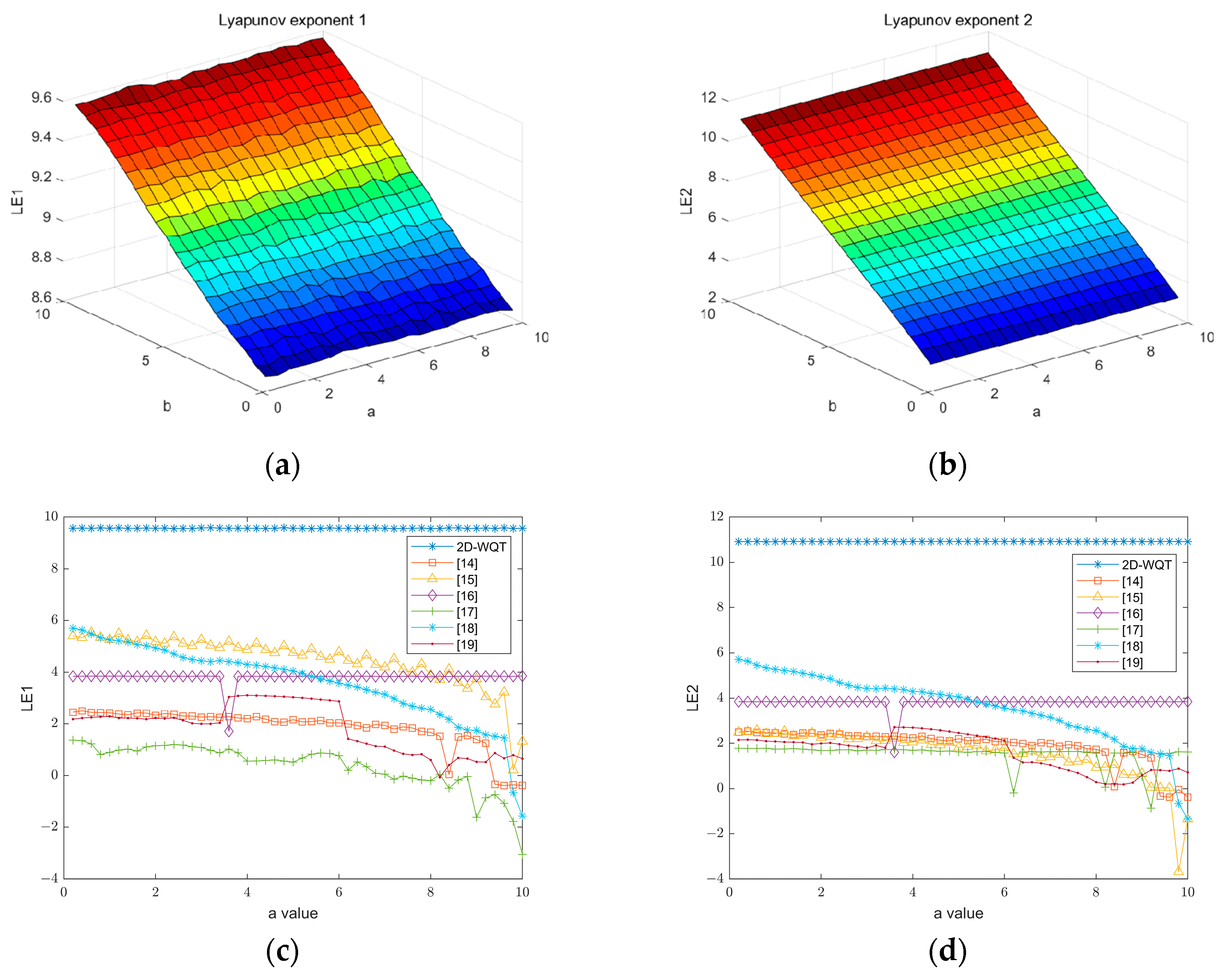
3. Chaos Performance Analysis

3.1. Analysis of Bifurcation Diagram

The bifurcation diagram is a collection of points in the chaotic mapping, and its trend can intuitively demonstrate the character of the chaotic system’s randomness [31]. The bifurcation diagram of 2D-WQT is depicted in Figure 4, which demonstrates that it exhibits clear chaotic behavior within the 0–10 range. In contrast to other chaos, this chaos has a broader chaos spectrum and a more uniform distribution.

3.2. Analysis of Phase Diagrams

The behavior of chaotic mapping dynamic systems can be effectively analyzed using phase space trajectory. Phase space is a high-dimensional space in which each dimension corresponds to a state variable of the system. The dynamic characteristics of the system can be intuitively observed by representing the state of the system at each moment as a location in the phase space and plotting the trajectory of the system’s evolution over time. In chaotic systems, these trajectories appear to be devoid of rules, demonstrating randomness and uncertainty. It is challenging to discern evident, predictable patterns from them. The 2D-WQT trajectory is illustrated in Figure 5. The other three images lack a distinct path in contrast to the logistic map, which has a clear cosine-like path. This is closely associated with the enhanced behavior of the WQT chaotic map, which is applicable in the field of encryption.

3.3. Analysis of Sensitivity

The sensitivity of high-dimensional chaotic systems is demonstrated by the fact that when the initial values or parameters are barely altered, the values obtained by the chaotic sequence should be entirely different, even under the same initial parameters. Figure 6 illustrates the primary modifications to the four parameters $a, b, x,$ and $y$ in the algorithm described in this paper when they change marginally. The small changes are designated as ${10}^{-14}$, respectively. There are evident distinctions in the chaotic system after $k=5$. The chaos we have developed is more sensitive than the two-dimensional chaos that currently exists with the same architecture.

3.4. Analysis of $LE$

The Lyapunov exponent $\left(LE\right)$ is frequently employed in the description of chaotic systems [32]. The specific formula for a two-dimensional discrete-time dynamical system that is described by a graph is as follows:

$$X_{n+1}=F\left(X_n\right),$$

(4)

The Lyapunov index is determined by calculating the Jacobian matrix $J\left(x_i,y_i\right)$ of the function mapping Fat at each point $x_n,y_n$. This matrix is used to describe the derivative matrix of the local linearization of the system in the state space of a nonlinear dynamic system, where $X_n={{(x}_n,y_n)}^T$ represents the state of the system at the time step $n$. The particular Jacobian matrix is as follows:

$$J\left(x_i,y_i\right)=\left({\displaystyle \genfrac{}{}{0pt}{}{\frac{\partial f_1(x_i,y_i)}{\partial x_i}}{\frac{\partial f_2(x_i,y_i)}{\partial x_i}}}{\displaystyle \genfrac{}{}{0pt}{}{ \frac{\partial f_1(x_i,y_i)}{\partial y_i}}{ \frac{\partial f_2(x_i,y_i)}{\partial y_i}}}\right),$$

(5)

The Lyapunov exponents ${LE}_1$ and ${LE}_2$ are defined as

$${LE}_i=\underset{n\to \infty }{\lim }{\displaystyle \frac{1}{n}}\sum _{i=1}^{n-1}\ln \left|{\mathit{\lambda }}_{\mathit{i}}\left(J\left(x_i,y_i\right)\right)\right|,$$

(6)

The number of iterations that can be conducted is denoted by $n$, and the $i-th$ eigenvalue of the Jacobian matrix $J\left(x_i,y_i\right)$ is represented by ${\lambda }_i$. The Lyapunov exponent ${LE}_1$ and the Lyapunov exponent ${LE}_2$ in the chaotic map denote the $LEs$ in distinct orientations. The sensitivity of the nonlinear dynamic system to the initial conditions in multiple dimensions, rather than just the exponential separation in one direction, is demonstrated by the requirement that a hyperchaotic system have at least two positive Lyapunov exponents. The proposed chaotic system, as illustrated in Figure 7, is a hyperchaotic system, as it contains two or more positives $LEs$. In contrast to other chaotic systems, this chaotic system has a significantly higher $LE$ index and a more stable $LE$. This indicates that the chaotic system has a larger chaotic interval and can be employed for image encryption, meeting the encryption requirements. The results of the comparison with other pertinent indicators in the literature are presented in

Table 1. Comparison of chaos mapping indicators.

Title	${\mathit{L}\mathit{E}}_1$	${\mathit{L}\mathit{E}}_2$	SE	PE
WQT	9.5658	10.9239	2.3332	0.99903
[14]	1.9	1.8481	1.3982	0.96811
[15]	4.4839	1.549	1.807	0.99383
[16]	3.8005	3.7984	0.90858	0.99865
[17]	1.844	1.6131	1.3408	0.97261
[18]	0.37197	1.5189	0.49676	0.85285
[19]	3.5989	3.6037	1.592	0.98177

.

3.5. SE Analysis

Sample entropy (SE) [33] is a novel approach to assessing the complexity of test time series by utilizing approximate entropy to characterize the output similarity of dynamic systems. We define the sample entropy calculation formula for an m-dimensional time series as follows:

$$SE(m,r,N)=-log{\displaystyle \frac{A}{B}},$$

(7)

The chaotic behavior of the system is more complex, and the regularity of the system is reduced as the SE value increases through calculation. The potential for the sequence to produce a novel pattern is suggested by the change in dimension. Figure 8 illustrates the sample entropy comparison under various parameters. The chaotic sequence’s regularity decreases, and its complexity increases significantly as SE increases, suggesting that it is a reasonable choice for image encryption.

3.6. PE Analysis

The complexity and nonlinear characteristics of a time series can be analyzed using permutation entropy (PE) as an indicator. By contrasting the local arrangement patterns of data points in the time series, it assesses the system’s complexity and randomness. It is a more sensitive method of measuring time series complexity than sample entropy [34]. By dividing the time series into non-overlapping subsequences and calculating the frequency of occurrence of the arrangement patterns in these subsequences, the complexity and randomization of the sequence are assessed. The permutation entropy method is capable of detecting more subtle changes because it treats the same number as various combinations in different permutations. A high permutation entropy value suggests that the patterns in the time series are diversified, and the sequence is more complex and random. Conversely, a low permutation entropy value suggests that the pattern in the sequence is more straightforward and more predictable, and the system behavior is more simple and orderly. Figure 9 illustrates the comparison of the permutation entropy of the chaotic mapping and 2D-WQT. The chaotic performance is improved, and the complexity increases when the permutation entropy is near 1. The permutation entropy of the 2D-WQT chaotic mapping is not significantly affected by parameter changes in the range of (0, 10) and can be stabilized at 1. This indicates that the chaotic effect is more ideal, demonstrating that the system has more complex dynamic behavior and better nonlinear characteristics, as evidenced by the image. The average permutation entropy of each chaotic mapping is also provided. Although the permutation entropy of numerous chaotic mappings exceeds 0.99, the permutation entropy of WQT is slightly higher than that of other chaotic mappings. This indicates that, despite the possibility of fluctuations in the parameters of WQT, its permutation entropy remains at the optimal level.

3.7. Spider Diagram Analysis

Spider diagrams are frequently employed in the analysis and research of chaotic systems to examine the iterative process of discrete dynamic systems. The spider diagram has attained a stable or fixed point when it converges to a specific point. The system is currently in a stable condition. The system demonstrates periodicity and a periodic orbit if the spider diagram indicates a state of cyclic reciprocation between multiple points. As shown in Figure 10, the points drawn in red are the trajectory distribution of the chaotic system in the phase space. The chaotic system enters a chaotic state when the spider diagram displays irregular and non-periodic behavior. This self-similarity or irregular structure results in the system becoming highly sensitive at this point, and the iterative trajectory does not converge, suggesting that chaos has a strong robustness.

3.8. NIST Randomness Test

The National Institute of Standards and Technology (NIST) conducts tests to assess the quality of random number generators. Subsequently, it employs the results to determine the suitability of chaotic systems for encryption schemes. The NIST SP800-22 statistical test suite comprises a total of 15 sub-tests. The significance level was established at 0.01 for each of the 15 sub-tests. The sequence is deemed to have passed the test when the p value obtained by the test is more significant than 0.01. In this article, we select the initial values of 0.714 and 0.528 to generate x-dimensional and y-dimensional sequences, respectively. We then construct a key generator using Formulas (8) and (9) to generate a 0–1 sequence that can be used for NIST testing, a total of 100. The sequence with a group length of ${10}^6$ was evaluated.

Table 2. NIST result.

Subset	X		Y
	p-Value	Proportion	p-Value	Proportion
Frequency	0.191687	99/100	0.779188	99/100
Block Frequency	0.048716	100/100	0.275709	100/100
Cumulative Sums	0.334538	99/100	0.719747	99/100
Runs	0.108791	99/100	0.004981	99/100
Longest Run	0.236810	99/100	0.759756	100/100
Rank	0.419021	99/100	0.798139	100/100
FFT	0.911413	100/100	0.202268	100/100
Non-Overlapping	0.779188	100/100	0.102526	98/100
Overlapping	0.798139	100/100	0.779188	100/100
Universal	0.025193	99/100	0.834308	99/100
Approximate Entropy	0.334538	98/100	0.115387	100/100
Random Excursions	0.304126	99/100	0.911413	98/100
Random Excursions Variant	0.229900	70/70	0.517442	61/61
Serial	0.450564	70/70	0.452799	61/61
Linear Complexity	0.030806	98/100	0.759756	98/100

illustrates the outcomes of the examination. The sequence’s randomness is demonstrated by the fact that all of its criteria pass.

$$\left\{\begin{array}{c}q\left(x_i\right)=mod\left({x^{\prime }}_i\cdot {10}^{10}, 1\right)\\ q\left(y_i\right)=mod\left({y^{\prime }}_i\cdot {10}^{10}, 1\right)\end{array},\right.$$

(8)

$$\left\{\begin{array}{c}\left\{\begin{array}{c}s\left(x_i\right)=0, 0\le q\left(x_i\right)\le 0.5\\ s\left(x_i\right)=1, 0.5<q\left(x_i\right)\le 1\end{array}\right.\\ \left\{\begin{array}{c}s\left(y_i\right)=0, 0\le q\left(y_i\right)\le 0.5\\ s\left(y_i\right)=1, 0.5<q\left(y_i\right)\le 1\end{array}\right.\end{array}\right.,$$

(9)

4. Encryption and Decryption Algorithms

4.1. Key Generation

The cryptographic system is incomplete without the key. The manner in which it is configured guarantees the secure transmission and reception of messages. Concurrently, it is capable of effectively defending against brute force attacks. At this juncture, we amalgamate the attributes of the original image and implement the outcomes produced by the SHA-512 algorithm. Using these results, we can obtain the initial parameter values of 2D-WQT through operations, thereby generating the chaotic sequence $S_1\cdots S_k$ that is required for subsequent operations. The key generation procedure is illustrated in Algorithm 1.

Step 1: Hash value generation

The encrypted image can be inputted into the SHA-512 algorithm to obtain a 512-bit hash value, with each 8-bit group representing a group. The resulting hash value is $H=H(\mathrm{1,2},\cdots ,64)$. Then, in order to facilitate the ensuing generation of initial values, we convert it from hexadecimal to decimal. Specifically, the operation function is as follows:

$$H^{\prime }=hex2dec\left(H\right),$$

(10)

Step 2: Initial value generation

The encryption method in this paper necessitates four distinct chaotic time series. Consequently, six distinct sets ($x,y,Lt,a,b,$ and $c$) must be generated for the succeeding encryption diffusion steps, each of which is based on the same plaintext image. The hash values $H^{\prime }\left(1\right),H^{\prime }\left(2\right),\cdots H\prime \left(64\right)$ are used to determine the initial value of the 2D-WQT chaotic map. The detailed calculation steps are provided in Algorithm 1.

Algorithm 1. Key generation process

$\mathrm{Input}: H^{\prime }\left(1\right),H^{\prime }\left(2\right),\cdots H\prime \left(64\right)$; $\mathrm{Output}: x$$,y$$,Lt$$,a$$,b$$,c$, 1.   $x_1=mod(H\prime (7)\times H\prime (9)\times H\prime \left(11\right)/e,1)$; 2.    $y_1=mod(\min \left(H^{\prime }\left(13\right),\cdots H^{\prime }\left(15\right)\right)⨁\max \left(H^{\prime }\left(17\right),\cdots H^{\prime }\left(19\right)\right)/\pi ,1$); 3.     ${Lt}_1=mod(\min \left(H^{\prime }\left(21\right),\cdots H^{\prime }\left(23\right)\right)\times \max \left(H^{\prime }\left(25\right),\cdots H^{\prime }\left(27\right)\right)\times e\times \pi ,1$); 4.   $x_2=mod(\left(H^{\prime }\left(29\right)\right)\oplus \left(H^{\prime }\left(31\right)\right)\oplus \left(H^{\prime }\left(33\right)\right)/e,1)$; 5.    $y_2=mod(\max \left(H^{\prime }\left(35\right),\cdots H^{\prime }\left(37\right)\right)⨁\min \left(H^{\prime }\left(39\right),\cdots H^{\prime }\left(41\right)\right)/\pi ,1$); 6.     ${Lt}_2=mod(\max \left(H^{\prime }\left(43\right),\cdots H^{\prime }\left(45\right)\right)\times \min \left(H^{\prime }\left(47\right),\cdots H^{\prime }\left(49\right)\right)\times e\times \pi ,1$); 7.   $a=mod(\min \left(H^{\prime }\left(4\right),\cdots H^{\prime }\left(6\right)\right)\times \min \left(H^{\prime }\left(8\right),\cdots H^{\prime }\left(10\right)\right),10)$; 8.    $b=mod(\max \left(H^{\prime }\left(14\right),\cdots H^{\prime }\left(16\right)\right)\times \max \left(H^{\prime }\left(18\right),\cdots H^{\prime }\left(20\right)\right),10)$; 9.     $c=mod(\max \left(H^{\prime }\left(24\right),\cdots H^{\prime }\left(26\right)\right)\times \min \left(H^{\prime }\left(28\right),\cdots H^{\prime }\left(30\right)\right),10)$; 10.  End;

Step 3: Generation of a chaotic sequence

The iteration core of Algorithm 2 is the 2D-WQT chaotic mapping system, which is implemented using the initial values $x,y,Lt$, as well as the control parameters $a,b,$ and $c$. It iterates $1000+M\times N\times 3$ times, discards the values of the first 1000 times, and subsequently generates a chaotic time series.

Algorithm 2. Chaotic sequence generation

$\mathrm{Input}: x_1$$,y_1$$,\mathrm{a}, \mathrm{b}, \mathrm{k}, L{t}_1$; $\mathrm{Output}: x$$, y$   Start;   $\mathrm{Get} x_1$$, y_1$, a, b;   for i = 1:k     $L{t}_{i+1}=4\times {Lt}_i\times \left(1-{Lt}_i\right);$     $x_{i+1}=i\times {{(x}_i)}^4\times \left(i+a\right)\times {{(y}_i)}^4+L{t}_{\left(i+1\right)} mod 1;$     $y_{i+1}=1-\cos \left({10}^b\times x_i\right)\times e^{\left({\displaystyle \frac{1}{c}}\times \left(-{{(x}_i)}^2\right)\right)}-\cos ({10}^b\times y_i)\times e^{\left({\displaystyle \frac{1}{c}}\times \left(-{{(y}_i)}^2\right)\right)})mod 1$;   End;   Stop;

The range of the chaotic sequence $S_1\cdots S_k$ required in the encryption phase is subject to change as the value $\beta$ is altered. The chaotic sequence that has been obtained at this time cannot be directly utilized for subsequent encryption operations; therefore, we preprocess it. The precise preprocessing formula is as follows:

$$S_k=floor({(x}_i-ceil\left(x_i\right)\times {10}^{12})) mod \beta ,$$

(11)

$$S_k=floor({(y}_i-ceil\left(y_i\right)\times {10}^{12})) mod \beta ,$$

(12)

The input value is rounded up using the $ceil(·)$ function, and the input value is rounded down using the $floor(·)$ function. The value $\beta$ is selected based on the value that will be used in the subsequent encryption process, and the encryption key of the final image is $S_k$. Among these, $x_i$ and $y_i$ are chaotic time series.

4.2. Lightweight Diffusion Algorithm

The fundamental purpose of diffusion is to alter the magnitude of pixel values. The robustness and anti-attack capabilities of the image can be significantly enhanced by the expansion of minor discrepancies in the image to the entire image, resulting in a completely distinct encrypted image. This paper’s lightweight diffusion algorithm has the ability to rapidly encrypt and modify the size of pixel values. Algorithm 3 that follows specifies the procedure.

Step 1: Acquire the chaos sequence

We must employ a chaotic sequence for dissemination in this step. The diffusion sequence $S_1$ can be generated by setting the value of $\beta$ to 256 in accordance with the processing requirements. Then, we group $S_1$ and reshape it into three chaotic matrices, each of which is $M\times N$.

Step 2: Merge channels

In this phase, we divide the three channels of the color image and obtain $M\times N$ matrices, $Q\prime \left(\theta ,\gamma ,\delta \right),Q\prime \left(\theta +1,\gamma ,\delta \right),$ and $Q\prime \left(\theta +2,\gamma ,\delta \right)$, respectively. Next, we combine them to produce a three-dimensional layer for subsequent processing.

Step 3: Initial diffusion

A chaotic matrix of the same size as the original image is obtained through the first stage. This chaotic matrix and the original channel are then subjected to a diffusion operation. The pseudo-code contains the diffusion phase. The new elements are obtained as the pixel values following the initial diffusion upon completion of the operation.

Step 4: Diffusion within the channel

In this operation, we employ the $M\times N\times 3$ three-dimensional matrix that was obtained after preliminary processing and combine the matrix operation characteristics to perform batch processing on all elements. Specifically, we alternately diffuse the three channels of $Q\prime \left(\theta ,\gamma ,\delta \right), Q\prime \left(\theta +1,\gamma ,\delta \right)$, and $Q\prime \left(\theta +2,\gamma ,\delta \right)$; the processing is conducted in a sequential manner, and the specific formula is as follows. The processing efficiency is enhanced by the use of matrix-vector operations instead of for loops, which can significantly enhance the calculation efficiency to obtain the rapid diffusion effect.

$$\left\{\begin{array}{c}Q\prime \prime \left(\theta ,\gamma ,\delta \right)=Q\prime \left(\theta ,\gamma ,\delta \right)\oplus Q\prime \left(\theta +1,\gamma ,\delta \right)⨁\theta \hfill \\ Q\prime \prime \left(\theta +1,\gamma ,\delta \right)=Q\prime \left(\theta +1,\gamma ,\delta \right)\oplus Q\prime \left(\theta +2,\gamma ,\delta \right)⨁\gamma \hfill \\ Q\prime \prime \left(\theta +2,\gamma ,\delta \right)=Q\prime \left(\theta +2,\gamma ,\delta \right)\oplus Q\prime \prime \left(\theta +,\gamma ,\delta \right)⨁\delta \hfill \end{array}\right.,$$

(13)

Step 5: Final image generation

The final encrypted image $C\prime$ is generated by recombining the three-layer matrices $Q\prime \prime \left(\theta ,\gamma ,\delta \right),Q\prime \prime \left(\theta +1,\gamma ,\delta \right),Q\prime \prime \left(\theta +2,\gamma ,\delta \right)$ after two rounds of diffusion.

For the sake of clarity, let us consider the $4\times 4\times 3$ color image $Q1$ as an illustration. Subsequently, we will implement a diffusion operation with the chaotic sequence $x_1$ that was generated to produce the diffused image $Q2$. In Figure 11, the process is illustrated in detail: Each block represents a different channel, and each small grid above represents the size of each pixel block value, and the above operations are performed separately.

Algorithm 3. Lightweight Diffusion Algorithm

$\mathrm{Input}: S_1$$, \mathrm{I}; S_1$ is generated by 2D-WQT, I is the Initial image. $\mathrm{Output}: x$$, I_{ciped}$ 1.   Start; 2.   Begin; 3.   I_Red = double(I1(:)); I_Green = double(I2(:)); I_Blue = double(I3(:)); 4.   Key_R = round(Key_R); Key_G = round(Key_G); Key_B = round(Key_B); 5.   I_Red_Cip = mod((I_Red+ Key_R),256); 6.    I_Green_Cip = mod((I_Green+ Key_G),256); 7.     I_Blue_Cip = mod((I_Blue+ Key_B),256); 8.   I_Red_Cip = bitxor(I_Red_Cip, I_Green_Cip); 9.    I_Green_Cip = bitxor(I_Green_Cip, I_Blue_Cip); 10.     I_Blue_Cip = bitxor(I_Blue_Cip, I_Red_Cip); 11.   End; 12.   Stop;

4.3. Roulette Coordinate Scrambling

The correlation between pixels in the image is not significantly disrupted by diffusion alone; however, the scrambling operation can significantly alter the connection between adjacent pixels. Consequently, at this juncture, we developed a novel roulette coordinate selector that, in conjunction with waveform scrambling, enabled us to implement global cross-channel scrambling on the diffused image $C\prime$. Algorithm 4 specifies the operation process:

Step 1: Chaotic sequence preprocessing

The chaotic sequence that is obtained is preprocessed to simplify subsequent operations and calculations. Initially, the chaotic sequence $y_1$ is operated to produce an arbitrary number between 1 and 3, which represents the three channels, respectively. Subsequently, the chaotic sequences $x_2$ and $y_2$ are operated to produce an arbitrary integer between 1 and N, which represents the width of the image $P$. Formulas (14)–(16) illustrate the precise procedure.

$$S_2=mod(floor({(y}_1-ceil\left(y_1\right)\times {10}^{12}\left)\right),3),$$

(14)

$$S_3=mod(floor({(x}_2-ceil\left(x_2\right)\times {10}^{12}\left)\right),M),$$

(15)

$$S_4=mod(floor({(y}_2-ceil\left(y_2\right)\times {10}^{12}\left)\right),N),$$

(16)

Algorithm 4. Roulette coordinate scrambling algorithm

Input: Image I of size M × M and secret keys Sec_key, Sec_key2, Sec_key3 Output: Scrambled image I   1. Start;   2. Define traversal_order as an empty list;   3. For each row j from 1 to M:   4.    If j is odd:   5.      Append all positions (j, k) for k = 1 to M to traversal_order;   6.    Else:   7.      Append all positions (j, k) for k = M down to 1 to traversal_order;   8. End For   9. For i = 1 to 3:   10.    For each position (j, k) in traversal_order:   11.      temp = I(j, k, i);   12.      index = (i − 1) × M × M + M × (j − 1) + k;   13.      I(j, k, i) = I(Sec_key(index), Sec_key2(index), Sec_key3(index));   14.      I(Sec_key(index), Sec_key2(index), Sec_key3(index)) = temp;   15.    End For   16. End For   17. End;   18. Stop;

Step 2: Waveform extraction

We employ a waveform approach to extract image elements in order to disrupt the correlation between adjacent pixels of the image. This can effectively disrupt the correlation between adjacent pixels at the periphery of the image, thereby preparing the image for subsequent processing.

Step 3: Scramble the roulette coordinates

The pixel block corresponding to the $3\times M\times N$ roulette coordinates that have been obtained is exchanged with each element on the original image in the order in which they were extracted from the waveform until all pixel blocks have completed an exchange. Formula (17) illustrates the precise procedure:

$$\left\{\begin{array}{c}temp=Q\prime \prime \left(\theta ,\gamma ,\delta \right)\hfill \\ Q\prime \prime \left(\theta ,\gamma ,\delta \right)=Q\prime \prime \left(S_k\right(i,j,t\left)\right)\hfill \\ Q\prime \prime \left(S_k\right(i,j,t\left)\right)=temp\hfill \end{array}\right.,$$

(17)

For the sake of clarity, consider the $4\times 4\times 3$ color image $Q2$ that is generated after the diffusion step. The chaotic sequence $y_1,x_2,y_2$ generates the roulette coordinates. The pixels that correspond to $Q2$ are scrambled according to the cells of the matching coordinates in the roulette coordinates, starting from $Q2 (\mathrm{1,1},1)$. This operation is performed in sequence until all pixel blocks are scrambled to obtain the scrambled three-dimensional image $Q3$. Figure 12 illustrates the precise procedure:

4.4. Overall Image Encryption Algorithm

In order to achieve secure and effective encryption of images, our algorithm is divided into several stages, including key generation, chaotic sequence generation, lightweight diffusion scheme, and three-dimensional roulette waveform scrambling, as a result of the aforementioned detailed encryption process. We present a flowchart of the encryption process, as illustrated in Figure 13, to facilitate a more intuitive understanding of the process.

4.5. Decryption Algorithm

The decryption algorithm reverses the encryption algorithm. After the sending party transmits the encrypted picture and key to the receiver, the decryption algorithm generates a chaotic sequence $S_1\cdots S_4$ through the key. The decrypted image can be obtained by carrying out the reverse diffusion operation on the encrypted image and the reverse process of the three-dimensional roulette coordinate scrambling via the chaotic sequences. Figure 14 illustrates the decryption algorithm’s sequence chart.

5. Experimental Results

The efficacy of this image encryption scheme was assessed using color images of $256\times 256,512\times 512,1024\times 1024$ sizes in this experiment. An AMD Ryzen 7 5800H 16G platform and NVIDIA GeForce RTX 3050 Laptop GPU 12G graphics card (Lenovo (Beijing) Co., Ltd. Made in China Guangdong Shenzhen) were employed in this experiment. Our pertinent experimental findings are as follows.

5.1. Algorithm Feasibility Verification

Figure 15 illustrates the encrypted image in question. It is evident that the encrypted image can effectively conceal the original image. It is challenging for the unaided eye to obtain effective information, as the encrypted image displays noise-like information. Simultaneously, the lossless original image can be obtained by decrypting the encrypted image, which further establishes the robustness of our encryption algorithm and guarantees the effective protection of the image’s information security.

5.2. Histogram Analysis

The histograms of the plaintext image and the encrypted image are compared in Figure 16. This demonstrates that the histogram of the encrypted image is entirely distinct from that of the ordinary image. The histogram distribution of the original plaintext image may align with the pixel feature distribution of the image, whereas the histogram of the encrypted image is nearly uniformly distributed. This suggests that the encrypted image has a more average and random distribution feature. This shows that the encryption algorithm is highly effective, greatly improving its ability to resist statistical analysis and other forms of attacks.

5.3. Key Space Analysis

The key space refers to the entire number of potential keys. The key space of a security chaos-based encryption of images algorithm should transcend $2^{120}$ [35]. The encryption algorithm’s resistance to brute force decryption is enhanced by the size of its key space. Consequently, in order to mitigate the danger of brute force attacks that may arise as a result of the escalating computing power and performance of computers, the key space should be as expansive as feasible under the circumstances. In this algorithm, two sets of keys must be transmitted to the recipient. In light of the aforementioned two scenarios, we are of the opinion that the assailant requires only one set of keys to be broken in order to accomplish their objective. Consequently, the key space should be selected as a set of keys with a reduced key space. Consequently, the key space of the algorithm proposed in this paper should be ${ 2}^{(52\times 6)}\times 1000\approx { 2}^{322}$, which is larger than $2^{120}$.

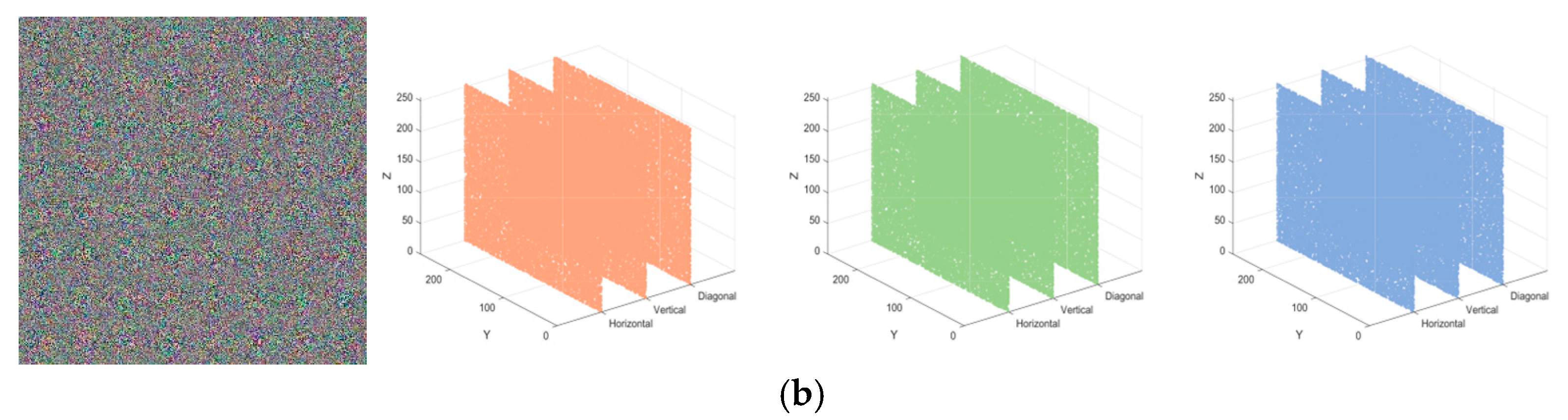
5.4. Correlation Analysis

The horizontal, vertical, and diagonal directions are the primary reflections of the correlation of zero-pixel images. Better results in resisting statistical attacks can be achieved when the encrypted image has minimal correlation in each of these three directions. The correlation’s precise calculation formula is as follows:

$$E(x)={\displaystyle \frac{1}{N}}{\sum }_{i=1}^N\left(x_i\right),$$

(18)

$$D(x)={\displaystyle \frac{1}{N}}\sum _{i=1}^N{\left(x_i-E\left(x_i\right)\right)}^2,$$

(19)

$$cov(x,y)={\displaystyle \frac{1}{N}}\sum _{i=1}^N(x_i-E(x_i\left)\right)(y_i-E(y_i\left)\right),$$

(20)

$$r_{xy}={\displaystyle \frac{cov(x,y)}{\sqrt{D\left(x\right)}\sqrt{D\left(y\right)}}}$$

(21)

where $cov\left(x,y\right)$ represents the covariance, $E\left(x\right)$ represents the mean, and $D\left(x\right)$ represents the variance.

The correspondence between the plaintext and ciphertext in three directions of 4.2.07 is illustrated in Figure 17. The figure clearly demonstrates that the correlation between the channels of the original image is highly significant and distributed in a diagonal pattern, indicating a strong correlation between adjacent pixel blocks. This is one of the reasons why images can be used to communicate information to us. Our objective is to disrupt this correlation. In order to achieve the effect of fuzzy information transmission, an exceptional algorithm can minimize the correlation of images to the greatest extent feasible. This method effectively disrupts the structure and features of the image, rendering it exceedingly challenging to analyze and decrypt encrypted images. By inspecting the correlation image of the encrypted image, it is evident that the correlation distribution is more uniform and random. The correlation coefficients of the ciphertext image 4.2.07 in the horizontal direction are 0.0031, 0.0046, and −0.0111, respectively, as determined by the formula mentioned above. The correlation coefficients in the vertical direction are −0.0006, 0.0053, and −0.0080, as determined by the same formula. For the image of the ciphertext in the diagonal direction, the correlation coefficients are 0.0041, −0.0053, and −0.0062, separately. The correlation has decreased markedly and is poised to approach the optimal value of 0 when contrasted with the original image.

Table 3. Image correlation evaluation.

Images	Size	Channel	——	Horizontal	Vertical	Diagonal
House	$512 \times$$512 \times$3	R	Original	0.95483	0.95736	0.92146
			This paper	−0.00304	0.00322	−0.006822
		G	Original	0.93696	0.94352	0.88982
			This paper	−0.00171	−0.0024019	−0.014512
		B	Original	0.97119	0.96683	0.94281
			This paper	−0.00553	−0.004458	−0.00672
Lena	$512 \times$$512 \times$3	R	Original	0.9758	0.9872	0.9648
			This paper	−0.0015	0.0035	−0.00016
			[17]	−0.0367	−0.0059	0.0182
			[36]	−0.0022	0.0057	0.00007
		G	Original	0.9760	0.9879	0.9638
			This paper	0.0010	0.00290	0.00757
			[17]	0.0030	0.0587	−0.0123
			[36]	0.0009	−0.0041	0.0038
		B	Original	0.95358	0.97332	0.93065
			This paper	−0.00067	−0.00312	−0.00152
			[17]	−0.0037	−0.0227	−0.0134
			[36]	0.0013	0.0017	0.0104

displays the comparative data with the results of other algorithms to enhance the representativeness of the analysis. It is evident that the algorithm proposed in this article has a calculated correlation coefficient that is lower than that of other algorithms, thereby substantially reducing the correlation between pixels. The algorithm proposed in this article is more secure and has a higher level of resistance to statistical attacks, as evidenced by the correlation.

5.5. Information Entropy Analysis

The degree of disorder in an image can be described by information entropy [37]. The information entropy of an image increases as the grayscale distribution becomes more uniform. Conversely, the information entropy decreases as the grayscale distribution becomes more unequal. The formula for calculating information entropy is as follows:

$$H=-{\sum }_{i=1}^{255}p\left(x_i\right){log}_{2}p\left(x_i\right),$$

(22)

where $p\left(x_i\right)$ denotes the probability of each event or result $x_{i }$; if the H value of the encrypted image is nearer to 8, the encryption effect is more effective for 256-level grayscale images. The plaintext and encrypted images’ information entropy values are presented in

Table 4. Information entropy analysis.

Images	Ciphertext			Plaintext
	R	G	B	R	G	B
4.1.05	6.4311	6.5389	6.5389	7.9973	7.9974	7.9974
4.1.06	7.2104	7.4136	7.4136	7.9972	7.9974	7.9974
house	7.4156	7.2295	7.2295	7.9993	7.9993	7.9993
4.2.07	7.3388	7.4963	7.0583	7.9994	7.9993	7.9994
2.2.01	7.7575	7.3387	6.9561	7.9998	7.9998	7.9998

. It is evident that the information entropy value of the encrypted image is greater than that of the ordinary image. The information entropy comparison between the algorithm in this paper and other existing algorithms is presented in

Table 5. Comparison of information entropy.

Image	File	R	G	B
Lena-512	This paper	7.9994	7.9994	7.9994
	[38]	7.9992	7.9993	7.9993
	[39]	7.9992	7.9994	7.9993
	[40]	7.9975	7.9973	7.9973
Airplane-512	This paper	7.9994	7.9994	7.9994
Baboon-256	This paper	7.9982	7.9980	7.9980
Lena-256	This paper	7.9976	7.9978	7.9976
	[40]	7.9968	7.9970	7.9969
	[39]	7.9969	7.9971	7.9968

. This algorithm has a marginally higher information entropy than the existing algorithms. Consequently, this algorithm has the capacity to conceal a significant amount of information.

5.6. Differential Attack Analysis

The differential attack analysis is a method in which the attacker compares the difference between the plaintext image and the corresponding ciphertext image before and after the plaintext image is slightly altered. The resulting relationship between the plaintext image and the encrypted image is determined [41]. Two indicators are typically employed to assess differential attack resistance: the uniform average change intensity (UACI) and the pixel change rate (NPCR). The optimal values of NPCR and UACI are 33.4635% and 99.6094%, respectively. The definitions of NPCR and UACI are provided in Formulas (23)–(25):

$$NPCR={\displaystyle \frac{1}{M\times N}}\sum _{i=1}^M\sum _{j=1}^{N}D\left(i,j\right)\times 100\%,$$

(23)

$$UACI={\displaystyle \frac{1}{M\times N}}\sum _{i=1}^M\sum _{j=1}^N{\displaystyle \frac{\left|C_1\left(i,j\right)-C_2\left(i,j\right)\right|}{255}}\times 100\%,$$

(24)

$$D\left(i,j\right)=\left\{\begin{array}{c}1{,C}_1\left(i,j\right)\ne C_2\left(i,j\right)\\ 0{,C}_1\left(i,j\right)=C_2\left(i,j\right)\end{array}\right.,$$

(25)

The encrypted image $C_1(i,j)$ is obtained without altering the plaintext pixel value. The encrypted image, $C_2(i,j)$, is obtained by altering the plaintext pixel value. The image’s height and breadth are denoted by M and N, respectively. The NPCR and UACI are calculated to be 0.9961 and 0.3343, respectively, after the calculation, using the “Lena” image as an example. The NPCR and UACI of “4.2.07” are 0.9959 and 0.3264, respectively. The NPCR and UACI of “house” are 0.9960 and 0.3093, respectively. The calculated values of NPCR and UACI for all test images are presented in

Table 6. NPCR and UACL values of the encryption algorithm in this paper.

Images	NPCR (%)			UACI (%)
	R	G	B	R	G	B
4.1.05	99.5895%	99.6541%	99.5850%	29.2090%	31.2231%	32.3875%
4.1.06	99.7653%	99.6353%	99.6854%	32.1960%	34.1940%	32.6740%
house	99.5892%	99.5911%	99.6220%	30.1640%	31.2790%	31.2910%
4.2.07	99.5983%	99.5975%	99.6239%	30.1340%	33.9340%	33.8485%
2.2.01	99.6153%	99.6067%	99.6213%	32.2513%	32.1166%	29.9989%

. The algorithm’s NPCR and UACI values are nearly identical to the ideal values. Consequently, the algorithm is more resilient to differential assaults and has enhanced security.

5.7. Anti-Attack Test

The PSNR is employed to quantify the degree of similarity between the decrypted and original images. The quality of the image is improved as the PSNR value increases, as the difference between the decrypted and original images becomes reduced. MSE is employed to quantify the pixel difference between the decrypted and original images, which is indicative of the pixel-level error in the image. A lesser MSE indicates that the image is more effectively restored following a noise attack. PSNR and MSE are defined by Formulas (26) and (27):

$$MSE={\displaystyle \frac{\sum _{i=1}^M\sum _{j=1}^N{\left(P\left(i,j\right)-D\left(i,j\right)\right)}^2}{m\times n}}$$

(26)

$$PSNR=10\times {log}_{10}\left({\displaystyle \frac{{255}^2}{MSE}}\right)$$

(27)

Out of these, $P\left(i,j\right)$ is the original plaintext image, $D\left(i,j\right)$ is the decrypted image, and $m$ and $n$ denote the image’s height and width, respectively.

5.7.1. Numerous Noise Attacks

Cropping attacks and noise attacks are critical methods for assessing the anti-attack capabilities of image encryption algorithms in the field of image encryption. In order to determine whether the decrypted image can still maintain integrity and readability, they can artificially modify or obliterate encrypted images. The robustness and security of encryption algorithms can be quantified by combining these attacks with analytical indicators.

Noise attacks simulate interference or malicious attacks during image transmission by introducing random noise into encrypted images, such as Gaussian noise and salt-and-pepper noise. Noise attacks are designed to evaluate the encryption algorithm’s resilience to random interference. PSNR and MSE are frequently employed as metrics for noise attack analysis. The house’s devastation is depicted in Figure 18 after it was subjected to varying degrees of Gaussian noise and 5% salt-and-pepper noise.

The PSNR of the salt and pepper noise assault and the cropping attack are presented in

Table 7. PSNR result.

Attack	R Channel	G Channel	B Channel
Gauss Noise-0.05%	40.0711	15.9197	27.7382
Gauss Noise-0.5%	21.5603	12.2238	19.0879
Gauss Noise-1%	17.7555	11.2555	16.2279
Salt and pepper Noise	21.7271	18.5129	21.3983
Block Attack	15.4182	13.4958	17.3099
6.25% Shearing	21.5308	17.6211	20.2593
12.5% Shearing	17.9937	14.6785	17.3420
25% Shearing	15.2589	12.0405	14.2498
50% Shearing	11.9813	10.0532	11.1216

. Although the PSNR value decreases as the intensity of the cropping attack and salt-and-pepper noise attack increases, it still maintains a satisfactory level. This indicates that the ciphertext image is more secure during transmission and can more effectively withstand cropping attacks and noise attacks.

5.7.2. Clipping and Channel Missing

The cropping attack involves the partial cropping of the encrypted image, the removal or destruction of specific image regions, and the subsequent analysis of the decrypted image’s recovery. Channel loss refers to the loss of distinct locations within various channels. We selected encrypted images with one-sixteenth, one-eighth, one-quarter, and one-half loss, as illustrated in the figure. The figure illustrates the ultimate outcome of the decryption process. The subject can still be identified, and the decrypted image is still plainly visible, even after 50% of the data is lost. This demonstrates that the algorithm in this paper possesses a strong anti-attack capability and can effectively mitigate the effects of data loss assaults on the restored image. The impact of image recovery following varying degrees of cropping and blocking assaults is more intuitively illustrated in Figure 19 and Figure 20.

5.8. Chosen Plaintext Attack

The chosen plaintext assault is a prevalent attack model in the field of cryptography. The attacker encrypts a specific plaintext and attempts to analyze the ciphertext in order to decrypt the encryption algorithm or key. The encrypted images are obtained by selecting all-black and all-white images for encryption in this paper. The encrypted images are comparable to noise, and the three-dimensional histogram is a uniformly distributed cube with a correlation coefficient near zero. Figure 21 indicates that the algorithm proposed in this paper is capable of effectively mitigating selected plaintext attacks.

5.9. Analysis of Encryption Time

The computational efficiency of encryption is primarily determined by factors such as computing resources, implementation methods, and the characteristics of the selected encryption algorithm [42]. An encryption algorithm that can encrypt the same amount of data in less time demonstrates higher encryption efficiency under identical experimental conditions, including hardware, software platforms, and the encryption image. Using a 512 × 512 image as the reference, the average encryption time is calculated based on the experimental algorithm chosen for this study. By comparing the experimental results under the same conditions, as shown in

Table 8. Comparison of various image encryption algorithms in terms of their time complexity.

Algorithms	--	512 × 512	1024 × 1024
This article	Encryption	0.0621	0.2581
[43]	Encryption	0.5726	2.0181
[44]	Encryption	1.3676	3.0399
[45]	Encryption	2.2234	9.0013
This article	Decryption	0.1025	0.4271
[45] [44]	Decryption Decryption	2.3218 2.3772	9.1095 4.4680

, the encryption efficiency of our algorithm is demonstrated to be greatly improved.

6. Conclusions and Outlooks

This research presents a composite picture encryption framework utilizing a two-dimensional hyperchaotic system with DNA coding. Using multidimensional nonlinear coupling and dynamic perturbation mechanisms makes the chaotic key generator much safer and more reliable. The nonlinear properties of the W/Wavy function and the Quartic function are combined in a new two-dimensional hyperchaotic map called 2D-WQT. The logistic map is used as a dynamic perturbation factor. It has been shown through experiments that the system has double positive Lyapunov exponents ($LE₁=9.57$ and $LE₂$ = 10.92) when the parameters $a=\left(\mathrm{3.5,5.0}\right)$ and $b=\left(\mathrm{0.8,1.5}\right)$. Additionally, the sample entropy (SE $\approx$ 2.33) and permutation entropy (PE $\approx$ 0.999) are markedly superior to those of current chaotic systems. The dimension of its chaotic trajectory is 1.92 $\pm$ 0.03, confirming its significant complexity in the phase space. The suggested three-dimensional roulette bit-level scrambling technique overcomes the constraints of conventional pixel-level permutation. Cross-channel coordinate perturbation and a double-layer diffusion method are used to lower the correlation coefficient of pixels next to each other to 0.003 (horizontal), −0.0006 (vertical), and 0.004 (diagonal). When the encryption algorithm is combined with the dynamic key generated by the SHA-512 hash (key space ≥ $2^{200}$), it achieves nearly ideal values for NPCR (99.62%), UACI (33.46%), and information entropy (7.9994). It also shows strong resistance to cropping attacks (PSNR ≥ 15.25 dB) and noise attacks (MSE ≤ 32.25). Compared to similar algorithms (see refs. [43,44,45]), the time it takes to encrypt an image of size 512 $\times$ 512 is cut by 78.5% (0.0621 s), and it can encrypt and decrypt images of different resolutions (from 256 $\times$ 256 to 1024 $\times$ 1024) without any loss, meeting real-time requirements. Despite the substantial enhancements in chaotic features and encryption efficacy, certain optimization aspects remain. The existing 2D-WQT system exhibits hyperchaotic properties, but excessive iterations may constrain its sensitivity to parameters and resistance to degradation. In the future, it might be possible to look into making three- or four-dimensional chaotic mappings and adding tensor coupling methods to make dynamic behavior even less predictable.

References

1. Li, S.; Chen, G.; Cheung, A.; Bhargava, B.; Lo, K.T. On the design of perceptual MPEG-video encryption algorithms. IEEE Trans. Circuits Syst. Video Technol. 2007, 17, 214–223. [Google Scholar] [CrossRef]
2. Kaur, M.; Singh, S.; Kaur, M. Computational image encryption techniques: A comprehensive review. Math. Probl. Eng. 2021, 2021, 5012496. [Google Scholar] [CrossRef]
3. Kaur, M.; Singh, S.; Kaur, M.; Singh, A.; Singh, D. A systematic review of metaheuristic-based image encryption techniques. Arch. Comput. Methods Eng. 2021, 29, 2563–2577. [Google Scholar] [CrossRef]
4. Liang, Q.; Zhu, C. A new one-dimensional chaotic map for image encryption scheme based on random DNA coding. Opt. Laser Technol. 2023, 160, 109033. [Google Scholar] [CrossRef]
5. Shannon, C.E. Communication theory of secrecy systems. Bell Syst. Tech. J. 1949, 28, 656–715. [Google Scholar] [CrossRef]
6. Aihara, K.; Takabe, T.; Toyoda, M. Chaotic neural networks. Phys. Lett. A 1990, 144, 333–340. [Google Scholar] [CrossRef]
7. Xu, X.; Chen, S. Single neuronal dynamical system in self-feedbacked Hopfield networks and its application in image encryption. Entropy 2021, 23, 456. [Google Scholar] [CrossRef]
8. Zhou, Y.; Bao, L.; Chen, C.L.P. Image encryption using a new parametric switching chaotic system. Signal Process. 2013, 93, 3039–3052. [Google Scholar] [CrossRef]
9. Zhang, H.; Hu, H. An image encryption algorithm based on a compound-coupled chaotic system. Digit. Signal Process. 2024, 146, 104367. [Google Scholar] [CrossRef]
10. Li, C.; Gao, Y.; Lei, T.; Li, R.Y.M.; Xu, Y. Two independent offset controllers in a three-dimensional chaotic system. Int. J. Bifurc. Chaos 2024, 34, 2450008. [Google Scholar] [CrossRef]
11. Pankaj, S.; Dua, M. Chaos based medical image encryption techniques: A comprehensive review and analysis. Inf. Secur. J. A Glob. Perspect. 2024, 33, 332–358. [Google Scholar] [CrossRef]
12. Cao, C.; Sun, K.; Liu, W. A novel bit-level image encryption algorithm based on 2D-LICM hyperchaotic map. Signal Process. 2018, 143, 122–133. [Google Scholar] [CrossRef]
13. Toktas, F.; Erkan, U.; Yetgin, Z. Cross-channel color image encryption through 2D hyperchaotic hybrid map of optimization test functions. Expert Syst. Appl. 2024, 249, 123583. [Google Scholar] [CrossRef]
14. Teng, L.; Wang, X.; Yang, F.; Xian, Y. Color image encryption based on cross 2D hyperchaotic map using combined cycle shift scrambling and selecting diffusion. Nonlinear Dyn. 2021, 105, 1859–1876. [Google Scholar] [CrossRef]
15. Sun, J. 2D-SCMCI hyperchaotic map for image encryption algorithm. IEEE Access 2021, 9, 59313–59327. [Google Scholar] [CrossRef]
16. Hua, Z.; Zhu, Z.; Chen, Y.; Li, Y. Color image encryption using orthogonal Latin squares and a new 2D chaotic system. Nonlinear Dyn. 2021, 104, 4505–4522. [Google Scholar] [CrossRef]
17. Qiu, H.; Xu, X.; Jiang, Z.; Sun, K.; Xiao, C. A color image encryption algorithm based on hyperchaotic map and Rubik’s Cube scrambling. Nonlinear Dyn. 2022, 110, 2869–2887. [Google Scholar] [CrossRef]
18. Wang, Q.; Zhang, X.; Zhao, X. Color image encryption algorithm based on novel 2D hyper-chaotic system and DNA crossover and mutation. Nonlinear Dyn. 2023, 111, 22679–22705. [Google Scholar] [CrossRef]
19. Wang, X.; Chen, X.; Zhao, M. A new two-dimensional sine-coupled-logistic map and its application in image encryption. Multimed. Tools Appl. 2023, 82, 35719–35755. [Google Scholar] [CrossRef]
20. Wang, X.; Liu, P. A new full chaos coupled mapping lattice and its application in privacy image encryption. IEEE Trans. Circuits Syst. I Regul. Pap. 2021, 69, 1291–1301. [Google Scholar] [CrossRef]
21. Gao, Q.; Zhang, X. Multiple-image encryption algorithm based on a new composite chaotic system and 3D coordinate matrix. Chaos Solitons Fractals 2024, 189, 115587. [Google Scholar] [CrossRef]
22. Cao, P.; Teng, L. A chaotic image encryption algorithm based on sliding window and pseudo-random stack shuffling. Nonlinear Dyn. 2024, 112, 13539–13569. [Google Scholar] [CrossRef]
23. Xu, Y.; Tang, M. Color image encryption algorithm using DNA encoding and fuzzy single neurons. IEEE Access 2022, 10, 127770–127782. [Google Scholar] [CrossRef]
24. Alawida, M. A novel DNA tree-based chaotic image encryption algorithm. J. Inf. Secur. Appl. 2024, 83, 103791. [Google Scholar] [CrossRef]
25. Liu, X.D.; Chen, Q.H.; Zhao, R.S.; Liu, G.Z.; Guan, S.; Wu, L.L.; Fan, X.K. Quantum image encryption algorithm based on four-dimensional chaos. Front. Phys. 2024, 12, 1230294. [Google Scholar] [CrossRef]
26. He, J.; Zhu, H.; Zhou, X. Quantum image encryption algorithm via optimized quantum circuit and parity bit-plane permutation. J. Inf. Secur. Appl. 2024, 81, 103698. [Google Scholar] [CrossRef]
27. Zhang, Z.; Tang, J.; Zhang, F.; Huang, T.; Lu, M. Medical image encryption based on Josephus scrambling and dynamic cross-diffusion for patient privacy security. IEEE Trans. Circuits Syst. Video Technol. 2024, 34, 9250–9263. [Google Scholar] [CrossRef]
28. Wang, J.; Zhang, R.; Liu, J. Partial-privacy image encryption algorithm based on time-varying delayed exponentially controlled chaotic system. Nonlinear Dyn. 2024, 112, 10633–10659. [Google Scholar] [CrossRef]
29. Courrieu, P. The Hyperbell algorithm for global optimization: A random walk using Cauchy densities. J. Glob. Optim. 1997, 10, 37–55. [Google Scholar] [CrossRef]
30. Storn, R. Differrential evolution: A simple and efficient adaptive scheme for global optimization over continuous spaces. Tech. Rep. Int. Comput. Sci. Inst. 1995, 11. [Google Scholar] [CrossRef]
31. Xu, Y.; Liu, J.; You, Z.; Zhang, T. A Novel Color Image Encryption Algorithm Based on Hybrid Two-Dimensional Hyperchaos and Genetic Recombination. Mathematics 2024, 12, 3457. [Google Scholar] [CrossRef]
32. Zhou, R.G.; Sun, Y.J.; Fan, P. Quantum image Gray-code and bit-plane scrambling. Quantum Inf. Process. 2015, 14, 1717–1734. [Google Scholar] [CrossRef]
33. Zhao, X.; Liu, J.; Liu, H.; Zhang, F. Dynamic analysis of a one-parameter chaotic system in complex field. IEEE Access 2020, 8, 28774–28781. [Google Scholar] [CrossRef]
34. Bandt, C.; Pompe, B. Permutation entropy: A natural complexity measure for time series. Phys. Rev. Lett. 2002, 88, 174102. [Google Scholar] [CrossRef]
35. Alvarez, G.; Li, S. Cryptographic Requirements for Chaotic Secure Communications. arXiv 2003, arXiv:nlin/0311039. [Google Scholar]
36. Li, Z.; Peng, C.; Tan, W.; Li, L. A novel chaos-based color image encryption scheme using bit-level permutation. Symmetry 2020, 12, 1497. [Google Scholar] [CrossRef]
37. Mfungo, D.E.; Fu, X. Fractal-based hybrid cryptosystem: Enhancing image encryption with RSA, homomorphic encryption, and chaotic maps. Entropy 2023, 25, 1478. [Google Scholar] [CrossRef]
38. Wang, S.; Sun, B.; Wang, Y.; Du, B. Image encryption algorithm using multi-base diffusion and a new four-dimensional chaotic system. Multimed. Tools Appl. 2024, 83, 10039–10060. [Google Scholar] [CrossRef]
39. Khalil, N.; Sarhan, A.; Alshewimy, M.A. An efficient color/grayscale image encryption scheme based on hybrid chaotic maps. Opt. Laser Technol. 2021, 143, 107326. [Google Scholar] [CrossRef]
40. Li, X.; Sun, B.; Bi, X.; Yan, H.; Wang, L. A novel color image encryption algorithm based on cross-plane scrambling and diffusion. Mob. Netw. Appl. 2024, 29, 583–594. [Google Scholar] [CrossRef]
41. Xu, X.; Chen, S. An optical image encryption method using Hopfield neural network. Entropy 2022, 24, 521. [Google Scholar] [CrossRef] [PubMed]
42. Gao, S.; Zhang, Z.; Iu, H.H.C.; Ding, S.; Mou, J.; Erkan, U.; Toktas, A.; Li, Q.; Wang, C.; Cao, Y. A Parallel Color Image Encryption Algorithm Based on a 2D Logistic-Rulkov Neuron Map. IEEE Internet Things J. 2025. [Google Scholar] [CrossRef]
43. Wang, X.; Zhang, X.; Gao, M.; Tian, Y.; Wang, C.; Lu, H.H.C. A color image encryption algorithm based on hash table, hilbert curve and hyper-chaotic synchronization. Mathematics 2023, 11, 567. [Google Scholar] [CrossRef]
44. Xu, Y.Q.; Zhen, X.X.; Tang, M. Dynamical System in Chaotic Neurons with Time Delay Self-Feedback and Its Application in Color Image Encryption. Complexity 2022, 1, 2832104. [Google Scholar] [CrossRef]
45. Xu, C.; Zhang, Y.; Gu, Z. A novel color image encryption method based on sequence cross transformation and chaotic sequences. Eng. Lett. 2020, 28, 1088–1092. [Google Scholar]
Figure 1. W/Wavy function.
Electronics 14 01914 g001
Figure 2. Quartic function.
Electronics 14 01914 g002
Figure 3. The design path of 2D-WQT.
Electronics 14 01914 g003
Figure 4. Bifurcation diagrams: (a) x i and a ; (b) x i and b .
Electronics 14 01914 g004
Figure 5. Phase space trajectory: (a) x i , x i + 1 and x i + 2 ; (b) y i , y i + 1 and y i + 2 ; (c) x i   and   x i + 1 ; (d) x i , y i .
Electronics 14 01914 g005
Figure 6. Initial value sensitivity analysis: (a) a = 4 ; (b) b = 5; (c) x = 0.714; (d) y = 0.528.
Electronics 14 01914 g006
Figure 7. (a,b) 2D-WQT Lyapunov exponent diagram; (c,d) Lyapunov exponent comparison chart.
Electronics 14 01914 g007
Figure 8. Sample entropy.
Electronics 14 01914 g008
Figure 9. Permutation entropy.
Electronics 14 01914 g009
Figure 10. Cobweb plot: (a) x i   and   x i + 1 ; (b) y i   and   y i + 1 .
Electronics 14 01914 g010
Figure 11. Lightweight diffusion algorithm.
Electronics 14 01914 g011
Figure 12. Roulette coordinate scrambling algorithm.
Electronics 14 01914 g012
Figure 13. Image encryption process.
Electronics 14 01914 g013
Figure 14. Image decryption process.
Electronics 14 01914 g014
Figure 15. Encryption and decryption comparison of test objects: (a) 4.1.05 (256 × 256 × 3); (b) 4.1.06 (256 × 256 × 3); (c) house (512 × 512 × 3); (d) 4.2.07 (512 × 512 × 3); (e) 2.2.01 (1024 × 1024 × 3).
Electronics 14 01914 g015
Figure 16. Histogram of original image and encrypted image: (a) plaintext image; (b) histogram of (a); (c) ciphertext image; (d) histogram of (c).
Electronics 14 01914 g016
Figure 17. Correlation simulation results: (a) plaintext image, red plane, green plane, blue plane; (b) cipher image, red plane, green plane, blue plane.
Electronics 14 01914 g017aElectronics 14 01914 g017b
Figure 18. Gaussian noise: (a) 0.0005; (b) 0.005; (c) 0.01; (d) salt-and-pepper noise.
Electronics 14 01914 g018
Figure 19. Blocking attack: (a) 6.25% shear; (b) 12.5% shear; (c) 25% shear; (d) 50% shear.
Electronics 14 01914 g019
Figure 20. Blocking attack (channel missing).
Electronics 14 01914 g020
Figure 21. Encryption result of white and black images: (a) black image; (b) encrypted black; (c) white image; (d) encrypted white; (e) histogram of black; (f) histogram of encrypted black; (g) histogram of encrypted white; (h) histogram of white.
Electronics 14 01914 g021