A Tetris-Based Task Allocation Strategy for Real-Time Operating Systems

Abstract

Real-time constrained multiprocessor systems have been widely applied across various domains. In this paper, we focus on the scheduling algorithm for directed acyclic graph (DAG) tasks under partitioned scheduling on multiprocessor systems. Effective real-time task scheduling algorithms significantly enhance the performance and stability of multiprocessor systems. Traditional real-time task scheduling algorithms commonly rely on a single-heuristic parameter as the reference for task allocation, which typically results in suboptimal performance. Inspired by the Tetris algorithm, we propose a novel heuristic scheduling algorithm, named Tetris game scoring scheduling algorithm (TGSSA), that integrates multiple-heuristic parameters. The process of real-time DAG task scheduling on a multiprocessor system is modeled as a Tetris game. Through simulations of the worst-case response time (WCRT) analysis and observed average response times in RT-Linux, which is a frequently-used real-time operating system, our algorithm demonstrates superior performance, effectively improving the efficiency and stability of real-time operating systems.

1. Introduction

Real-time operating systems (RTOSs) are increasingly utilized in embedded systems across various domains, including edge computing, industrial automation, vehicle control systems, aerospace, medical devices, and the Internet of Things (IoT) [1,2,3,4,5]. These rapidly evolving technologies demand significant computational power, leading to the widespread deployment of RTOSs on multiprocessor platforms [6,7,8]. As technology continues to advance, the requirements for real-time performance and system reliability are becoming more stringent [9]. Task scheduling, a core function of RTOSs, has emerged as a critical area of research. Efficient task scheduling impacts system performance, response time, and the safety and stability of applications [10]. However, compared to single-processor systems, implementing real-time task scheduling on multiprocessor platforms presents greater complexity.

The primary goal of task scheduling in real-time systems is to ensure that critical tasks meet their deadlines, satisfying real-time constraints [6]. Depending on the scheduling strategy, scheduling methods can be categorized into static and dynamic approaches. Static scheduling determines the execution order of tasks during the design phase of the system, making it suitable for environments where task characteristics are well defined and remain stable [10,11]. Conversely, dynamic scheduling assigns tasks based on runtime conditions, offering greater flexibility and adaptability [4]. This approach is particularly effective in handling varying task loads and real-time priority adjustments.

Real-time tasks are characterized by stringent timing requirements. In hard real-time systems, missing a task deadline can have severe repercussions, such as jeopardizing aviation safety in flight control systems [6]. In soft real-time systems, while task deadline violations may not result in system failure, they can significantly degrade system performance [5]. Therefore, the primary objectives of task scheduling are to ensure adherence to timing constraints, optimize resource utilization, and maintain system stability and efficiency.

With the rise of multicore processors and cloud computing in recent years, task scheduling has encountered both new challenges and opportunities [3]. While multicore architectures enhance resource utilization, they also introduce issues such as task synchronization and competition for resources. Simultaneously, the growing adoption of edge computing and IoT has increased the need for scalable and efficient scheduling algorithms [12]. To address these challenges, researchers have developed innovative scheduling strategies, including priority-based scheduling, hybrid scheduling, and distributed scheduling. Moreover, there is a growing emphasis on the security and predictability of real-time task scheduling. As real-time systems are increasingly deployed in critical applications, ensuring their robustness and reliability under extreme conditions has become a key design consideration. Thus, modern research not only focuses on optimizing task completion rates and system responsiveness but also on enhancing system reliability and stability [12].

Traditional real-time scheduling theories have primarily focused on single-processor systems. However, with the advent of multiprocessor and multicore systems, the limitations of single-processor scheduling models have become apparent. Task scheduling in multicore processors is far more complex, requiring consideration of factors such as task allocation across processors, load balancing, task migration, and inter-task communication and synchronization. To address these challenges, researchers have proposed global, partitioned, and hybrid scheduling strategies that adapt traditional algorithms for multiprocessor environments. These approaches aim to achieve efficient resource utilization and flexible task distribution, meeting the evolving demands of modern real-time systems.

In real-time multiprocessor systems, most scheduling algorithms are based on single-heuristic parameters to allocate tasks, such as completion time, processor utilization, schedulability, etc. [12]. Different from previous research on real-time scheduling algorithms for multiprocessors, we draw inspiration from the Tetris algorithm and propose a new scheduling algorithm (TGSSA) with multiple-heuristic parameters through scoring the states of the scheduling progress. The main contributions can be summarized as follows:

• We innovatively abstract the task scheduling process into a Tetris game and propose a reliable task scheduling algorithm that can comprehensively consider multiple-heuristic parameters, by extending El Tetris, a classic Tetris playing algorithm, and combining it with task scheduling. Most existing algorithms are only able to consider a single-heuristic parameter.
• We not only conduct WCRT analysis on the results of the scheduling algorithm, but also conduct actual real-time task tests on Ubuntu 22.04 with real-time patch on AMD Ryzen 7 4800U.

The remainder of this paper is organized as follows. Section 2 introduces related work. Section 3 describes the system model and WCRT analysis method used in this paper. Section 4 and Section 5 introduce the new task allocation strategy. Section 6 reports experimental evaluations. Section 7 concludes this paper and discusses possible future work.

2. Related Work

In real-time task scheduling problems, tasks are often periodic, meaning that each task executes at regular intervals determined by its period. A crucial aspect of this model is determining the priority relationships among tasks to ensure proper scheduling.

Rate monotonic scheduling (RMS) is a widely used fixed-priority scheduling algorithm for periodic real-time tasks, especially in single-processor systems [13]. The key feature of RMS is that task priority is directly related to its period (or frequency): tasks with shorter periods are assigned higher priorities. RMS is a static priority scheduling method, operating under the assumption that the execution time of each task is known and all tasks are periodic. During the design phase, priorities are assigned to tasks and remain fixed throughout system operation. In practice, RMS operates efficiently by allowing the scheduler to interrupt the currently running task if a higher-priority task becomes ready. If the new priority of task is lower or equal, the current task continues execution.

In addition to RMS, other scheduling algorithms like earliest deadline first (EDF) and deadline monotonic scheduling (DMS) are also prevalent [7,13]. The EDF is a dynamic priority algorithm that, in theory, achieves up to 100% processor utilization on a single processor, outperforming RMS’s 69.3% utilization limit. However, RMS offers simpler implementation and greater predictability, making it a preferred choice in embedded systems with steady resource requirements. The EDF is more suited for environments with significant load fluctuations. The DMS, similar to RMS, assigns task priorities based on deadlines instead of periods. The RMS is best suited for systems where task periods are equal to deadlines, while DMS handles cases where these differ. As one of the most critical fixed-priority scheduling algorithms, RMS is simple, efficient, and optimally suited for fixed-priority systems, making it a trusted choice in many industrial and embedded applications. TGSSA is used for task partitioning on multiple processors, while RMS, DMS, and EDF are used for priority allocation on a single processor. TGSSA can increase the number of subtasks that can run at the same time, while single processor scheduling algorithms determine preemption on a single processor. They do not conflict with each other, and work together.

There are multiple ways to model task allocation, such as directed acyclic graph (DAG) [11], synchronous parallel task model [14], sporadic-based models [15], gang scheduling model [16], and fork-join task model [17]. For multiprocessor systems, task allocation strategies often employ heuristic algorithms to address DAG task allocation challenges. Casini et al. introduced a heuristic algorithm called Schedulability Testing Priority Assignment (STPA), which uses breadth-first search to allocate subtasks in a DAG across processors [18]. The STPA performs schedulability tests before assigning each subtask to ensure feasibility. If a subtask fails these tests across all processors, the algorithm deems the task set unschedulable. However, this method incurs high computational complexity and often struggles with low schedulability rates. Özkaya et al. proposed a clustering-based approach (BLM), but its effectiveness was limited in general scenarios [19]. Aromolo et al. categorized DAG tasks into heavy and light types, assigning heavy-task subtasks across all processors while restricting light-task subtasks to a single processor. While straightforward, this method can lead to underutilization of resources [12].

To improve efficiency, some researchers have adopted the principles of list scheduling algorithms, assigning priorities to subtasks within DAG tasks to facilitate allocation. He et al. introduced a list-based priority scheme for DAG subtasks, aiming to resolve parallelization conflicts through priority-based scheduling [12]. However, simple heuristic strategies in such methods often fail to deliver optimal results. Inspired by the multiheuristic parameter optimization techniques used in the Tetris algorithm (El Tetris), we propose a novel multiple-heuristic parameter real-time scheduling algorithm [20]. This approach aims to enhance task scheduling efficiency and improve overall system performance.

3. System Model

3.1. Task Execution Model

In task scheduling models, individual tasks are typically abstracted as DAGs [21,22]. In the system under study, a set of N DAG tasks, denoted as $\Gamma =\{{\tau }_1,{\tau }_2,\cdots ,{\tau }_N\}$, is scheduled on a real-time homogeneous computing platform. This platform consists of m homogeneous processors, denoted as $p_1,p_2,\cdots ,p_m$. Each DAG task can be represented as ${\tau }_i=(V_i,E_i,T_i,D_i,{\pi }_i)$, where $V_i$ is the set of subtasks (nodes), $E_i$ the edges, $T_i$ the arrival period, $D_i$ the relative deadline, and ${\pi }_i$ the fixed priority.

The set of subtasks of DAG ${\tau }_i$ is represented as $V_i=V_{i,1},V_{i,2},\dots ,V_{i,|V_i|}$, where $V_{i,j}$ denotes the j-th subtask of ${\tau }_i$. Each subtask is defined by its worst-case execution time (WCET) $C_{i,j}$ and the processor $P_{i,j}$ to which it is assigned. Specifically, $V_{i,j}=\langle C_{i,j},P_{i,j}\rangle$, where $C_{i,j}$ represents the WCET of the subtask and $P_{i,j}$ represents the processor on which the subtask is assigned to run.

An edge $e(V_{i,a},V_{i,b})$ represents a dependency from subtask $V_{i,a}$ to subtask $V_{i,b}$. $e(V_{i,a},V_{i,b})$ means that subtask $V_{i,b}$ can only begin execution after $V_{i,a}$ finishes execution. In this case, $V_{i,a}$ is considered the predecessor of $V_{i,b}$, and $V_{i,b}$ is considered the successor of $V_{i,a}$. We use $\mathbb{P}\left(V_{i,j}\right)$ and $\mathbb{S}\left(V_{i,j}\right)$ to represent the sets of predecessors and successors of subtask $V_{i,j}$, respectively [11]. For example, in the case of $V_{i,a}$ and $V_{i,b}$ mentioned above, $V_{i,a}\in \mathbb{P}\left(V_{i,b}\right)$ and $V_{i,b}\in \mathbb{S}\left(V_{i,a}\right)$.

If a subtask has no predecessors, i.e., $\mathbb{P}\left(V_{i,j}\right)=\varnothing$, it is called an entry subtask. If ${\tau }_i$ has multiple entry subtasks, a virtual entry subtask with a WCET of 0 is added to the DAG, along with edges from the virtual entry subtask to each of the entry subtasks. Similarly, if a subtask has no successors, i.e., $\mathbb{S}\left(V_{i,j}\right)=\varnothing$, it is called an exit subtask. If ${\tau }_i$ has multiple exit subtasks, a virtual exit subtask with a WCET of 0 is added to the DAG, along with edges from the exit subtasks to the virtual exit subtask [11].

In this paper, we simplify by assuming that $D_i=T_i$. To determine the period $T_i$, we introduce the utilization $U_i$ of DAG ${\tau }_i$ and the total WCET $Csu{m}_i={\sum }_{j=1}^{|V_i|}{C}_{i,j}$, so that $T_i=Csu{m}_i/U_i$. Further, by using U to represent the utilization of the entire set $\Gamma$, it can be calculated as $U={\sum }_{i=1}^N{U}_i$.

The priority ${\pi }_i$ of each task ${\tau }_i$ is fixed and determined by RMS in this paper. The detailed procedure for assigning priorities to the tasks in $\Gamma$ is presented in Section 2. Once the priorities are assigned, they remain fixed during execution. Additionally, due to the nature of RTOSs, a higher-priority subtask will preempt a lower-priority subtask if the higher-priority subtask is ready to execute. All subtasks of the same task ${\tau }_i$ share the same priority ${\pi }_i$, so no preemption occurs between subtasks of the same DAG task.

Figure 1 shows a DAG task ${\tau }_i$ with $Csu{m}_i=95$ and $T_i=D_i=100$. $V_{i,1}$ is an entry subtask. $V_{i,3}$, $V_{i,7}$, and $V_{i,8}$ are exit subtasks. Taking $V_{i,2}$ as an example, $<15,2>$ means that the subtask has a WCET of 15, and $P_{i,2}=2$. Then, we provide five definitions that will be used in the following algorithms.

First, a path ${\lambda }_{i,k}$ is a sequence $\{V_{entry}\to \cdots \to V_{i,s-1}\to V_{i,s}\cdots \to V_{exit}\}$ of subtasks in DAG task ${\tau }_i$. Any two adjacent subtasks in a sequence exist on adirected edge in $E_i$, i.e., $e(V_{i,s-1},V_{i,s})\in E_i$. At least one path exists in a DAG task, and $|{\lambda }_i|$ represents the number of paths in ${\tau }_i$.

Second, we define a processors set as $pr\left(B\right)$, where subtasks in set B will be executed on it. For example, the processors set $pr\left({\tau }_i\right)$ denotes subtasks in ${\tau }_i$ that will be executed on it.

Thrid, if the following two conditions are satisfied, the subtask $V_{i,s}$ is the indirect father subtask of $V_{i,t}$, and the subtask $V_{i,t}$ is the indirect child subtask of $V_{i,s}$:

• $e(V_{i,s},V_{i,t})$ is not included in the directed edges set $E_i$ of ${\tau }_i$.
• At least one directed path in ${\tau }_i$ connects $V_{i,s}$ and $V_{i,t}$.

Fourth, $len\left({\lambda }_{i,k}\right)$ denotes the WCET of the k-th path in ${\lambda }_i$.

Last, if $V_{i,j}$ and $V_{i,k}$ are not connected by any directed path, $V_{i,j}$ and $V_{i,k}$ is called a nondirect topological relationship, referred to as an NDT relationship.

3.2. RTA Analysis Strategy

In this subsection, we introduce a traditional WCRT analysis strategy, “response time algorithm” (RTA). For ${\tau }_i$, the WCRT is equal to the maximum WCRT within all directed paths and can be calculated by Equation (1) [23]:

$$R\left({\tau }_i\right)=\underset{k\in [1,|{\lambda }_i\left|\right]}{max}\left\{R\left({\lambda }_{i,k}\right)\right\}.$$

(1)

As shown in Equation (1), $R\left({\lambda }_{i,k}\right)$ represents the directed path ${\lambda }_{i,k}$’s WCRT. It can be calculated using Equation (2) [23]:

$$R\left({\lambda }_{i,k}\right)=len\left({\lambda }_{i,k}\right)+I_{high}\left({\lambda }_{i,k}\right)+I_i\left({\lambda }_{i,k}\right).$$

(2)

In Equation (2), $R\left({\lambda }_{i,k}\right)$ contains three parts. The first part $len\left({\lambda }_{i,k}\right)$ is the WCET of this path. The second part, $I_{high}\left({\lambda }_{i,k}\right)$, is high-priority interference caused by tasks $hp\left({\tau }_i\right)$. The third part $I_i\left({\lambda }_{i,k}\right)$ is self-interference, which is caused by the same subtasks in the DAG task ${\tau }_i$ but not in the path ${\lambda }_{i,k}$.

In schedulability test, a DAG task ${\tau }_i$ is schedulable if its WCRT is less than or equal to the deadline $D_i$. Furthermore, a set of DAG tasks $\Gamma$ is schedulable if all DAG tasks are schedulable. In practical scenarios, we are unable to obtain exact self-interference $I_i\left({\lambda }_{i,k}\right)$ and high-priority interference $I_{high}\left({\lambda }_{i,k}\right)$ before execution. Instead, we can explore $R\left({\lambda }_{i,k}\right)$’s upper bound $R^{ub}\left({\lambda }_{i,k}\right)$. The first part $len\left({\lambda }_{i,k}\right)$ represents the WCET of ${\lambda }_{i,k}$, which can be exactly calculated. Therefore, we can analyze the self-interference upper bound of $I_i\left({\lambda }_{i,k}\right)$ and the high-priority interference upper bound of $I_{high}\left({\lambda }_{i,k}\right)$ separately to obtain $R^{ub}\left({\lambda }_{i,k}\right)$.

3.2.1. High-Priority Interference

Among the subtasks of tasks with higher priority than ${\tau }_i$, only subtasks assigned to the same processor in $pr\left({\lambda }_{i,k}\right)$ can generate high-priority interference on ${\lambda }_{i,k}$. The total workload $Q_j\left({\lambda }_{i,k}\right)$ for ${\tau }_j$ in processors $pr\left({\lambda }_{i,k}\right)$ can be represented by the following Equation (3) [23]:

$$Q_j\left({\lambda }_{i,k}\right)=\sum _{p\in pr\left({\lambda }_{i,k}\right)\cap pr\left({\tau }_j\right)}\sum _{P_{j,t}=p}{C}_{j,t}.$$

(3)

The upper bound of high-priority interference $I_j^{ub}\left({\lambda }_{i,k}\right)$ generated by ${\tau }_j$ can be calculated by following Equation (4) [23]:

$$I_j^{ub}\left({\lambda }_{i,k}\right)=\lceil {\displaystyle \frac{R\left({\lambda }_{i,k}\right)+J_j}{T_j}}\rceil Q_j\left({\lambda }_{i,k}\right).$$

(4)

In Equation (4), $J_j$ can be calculated by the following Equation (5) [23]:

$$J_j=D_j-mi{n}_{p\in pr\left({\lambda }_{i,k}\right)\cap pr\left({\tau }_j\right)}\sum _{p_{j,t}=p}{C}_{j,t}.$$

(5)

3.2.2. Self-Interference

All subtasks in the same DAG task have the equivalent priority and can not preempt each other. For $V_{i,a}$ not in ${\lambda }_{i,k}$ and $V_{i,b}$ in ${\lambda }_{i,k}$, the subtask $V_{i,a}$ is a self-interference subtask of $V_{i,b}$ if the subsequent two conditions are satisfied:

• $V_{i,a}$ and $V_{i,b}$ are executed on the same processor.
• $V_{i,a}$ and $V_{i,b}$ are in an NDT relationship.

$self\left(V_{i,t}\right)$ represents the subtasks that will result in self-interference on $V_{i,t}$. Therefore, the subtasks that will result in self-interference on ${\lambda }_{i,k}$ can be represented by the following Equation (6) [23]:

$$self\left({\lambda }_{i,k}\right)={\cup }_{V_{i,t}\in {\lambda }_{i,k}}self\left(V_{i,t}\right).$$

(6)

Therefore, the upper bound of the self-interference can be calculated by Equation (7) [23]:

$$I_i^{ub}\left({\lambda }_{i,k}\right)=\sum _{V_{i,t}\in self\left({\lambda }_{i,k}\right)}{C}_{i,t}.$$

(7)

Based on Equations (2), (4) and (7), the WCRT of ${\lambda }_{i,k}$ can be calculated by the following Equation (8) [23]:

$$\begin{array}{c}\hfill R^{ub}\left({\lambda }_{i,k}\right)=len\left({\lambda }_{i,k}\right)+\sum _{V_{i,t}\in self\left({\lambda }_{i,k}\right)}{C}_{i,t}\\ \hfill +\sum _{{\tau }_j\in hp\left({\tau }_i\right)}\lceil {\displaystyle \frac{R^{ub}\left({\lambda }_{i,k}\right)+J_j}{T_j}}\rceil Q_j\left({\lambda }_{i,k}\right).\end{array}$$

(8)

In summary, we calculated the WCET, self-interference upper bound, and high-priority interference upper bound of the path ${\lambda }_{i,k}$ in the DAG, and combined these three upper bound analyses to obtain a formula for the WCRT upper bound of the path ${\lambda }_{i,k}$. $R^{ub}\left({\lambda }_{i,k}\right)$ exists on both sides of Equation (8), so the WCRT analysis result of the path can be obtained by iterative solution. The solution of Equation (8) represents the WCRT of directed path ${\lambda }_{i,k}$. Finally, we calculate the WCRT of all paths and find the maximum value to obtain the WCRT of the DAG task ${\tau }_i$.

4. Tetris-Based Allocation Model

Task partitioning and scheduling typically aim to minimize the WCRT of tasks to optimize system performance. When the number of processors is fixed at m, WCRT can be approximated by maximizing the parallelism between subtasks, subject to system constraints. In other words, the goal is to maximize the number of subtasks executed in parallel at any given time. This can be equated to the idea that, at any point in time, the more subtasks that are executed concurrently, the better. If at a given moment, m subtasks are being executed simultaneously, then the parallelism of the task at that moment has reached its upper bound. That is, even if additional subtasks are available for parallel execution, there will no longer be sufficient processors to accommodate them. Therefore, the ideal scenario we seek is to achieve this maximum level of parallelism as often as possible, ensuring that, at each moment, as many as m processors are actively executing tasks.

We construct a coordinate system with processor indexes on the horizontal axis and time t on the vertical axis. If a subtask $V_{i,j}$ is assigned to processor $P_{i,j}$, and executes from time $t_1$ to time $t_2$, the corresponding grid cells in the coordinate system at $P_{i,j}$ are marked on the horizontal axis, and between $t_1$ and $t_2$ on the vertical axis. In this context, the objective of ensuring that as many processors as possible are executing tasks at any given moment can be interpreted as filling as many cells as possible along a given vertical coordinate (time) within a particular column (processor).

Furthermore, each subtask can be considered as a block with a width of 1 and a height of $C_{i,j}$. The objective is to place each block into the appropriate column (processor) and row (start time) in such a way that as many rows as possible are filled.

The above process closely resembles the well-known game Tetris. In the exploration of the Tetris gameplay algorithm, Pierre Delacherie, Islam El-Ashi [20], and others introduced several key concepts related to the Tetris board.

• Landing height: The height where the piece is placed, which equals the height of the column plus half the height of the piece.
• Rows eliminated: The number of rows eliminated after the last piece is placed.
• Row transitions: The total number of row transitions. A row transition occurs when an empty cell is adjacent to a filled cell on the same row and vice versa.
• Column transitions: The total number of column transitions. A column transition occurs when an empty cell is adjacent to a filled cell on the same column and vice versa.
• Number of holes: A hole is an empty cell that has at least one filled cell above it in the same column.
• Well sums: A well is a succession of empty cells such that their left cells and right cells are both filled.

Theorem 1.

In the context of aperiodic tasks, higher processor utilization, more parallel execution time, and a higher number of removal rows in Tetris are all equivalent.

Proof. 

The WCET is fixed for a DAG task set, i.e., $Csum={\sum }_{i=1}^{N}Csu{m}_i={\sum }_{i=1}^N{\sum }_{j=1}^{|V_i|}{C}_{i,j}$ is fixed. From a timescale perspective, supposing the task set starts at $t=0$ and ends at $t=WCRT$, the parallel execution time at the k-th tick is denoted as $pa{r}_k=m-\left(thenumberofidleprocessors\right)$. In other words, $Csum={\sum }_{k=0}^{WCRT}pa{r}_k$. In this equation, $Csum$ is fixed, so larger $pa{r}_k$s means smaller WCRT. The removal rows in Tetris correspond to $pa{r}_k=m$; that is, there is no idle processor existing at this tick. Therefore, higher processor utilization, more parallel execution time, and a higher number of removal rows in Tetris are all equivalent.  □

It is evident that preemption caused by higher-priority tasks in periodic tasks does not alter the conclusions presented in Theorem 1.

Theorem 2.

The concepts of landing height, rows eliminated, row transitions, column transitions, holes, and wells are present in task scheduling problems, serving functions analogous to those in the Tetris game.

Proof. 

Landing height: In the Tetris game, when other factors are equal, players tend to allow a piece to land at a lower position. Similarly, in task scheduling, each subtask has a start time. When other factors are constant, users prefer to start the subtask as early as possible.

Rows eliminated: A key objective in Tetris is to eliminate as many rows as possible. In a multiprocessor system, when each processor is executing a task, the system utilization is maximized at that moment.

Row transitions and column transitions: In Tetris, players aim to minimize row and column transitions after the pieces have landed. In task scheduling, higher row and column transitions typically indicate greater imbalance in processor utilization and lower overall processor efficiency.

Holes: In Tetris, holes generally represent a series of cells that are difficult to utilize because rows above them must be cleared before they can be used. Therefore, players aim to avoid creating holes. In task scheduling, an increased number of holes often indicates lower processor utilization.

Wells: In Tetris, a well refers to a depression in the board that can potentially lead to the creation of holes in subsequent game steps. Players tend to minimize the formation of wells. Similarly, in task scheduling, it is desirable to minimize wells to prevent inefficiency in processor usage.  □

The task scheduling process differs from the actual Tetris game in several key aspects. Firstly, in the Tetris game, there are pieces of various shapes, while in task scheduling, there is only one type of piece consisting of a single column and multiple rows. The number of rows in this piece corresponds to the WCET of the respective subtask. Secondly, in the Tetris game, a piece can descend until it reaches an adjacent filled cell. In task scheduling, in addition to this constraint, the piece cannot extend beyond the completion time of its predecessors.

Despite these differences, it is evident that they do not cause a qualitative change in the concepts outlined in Theorem 2. The impact of each concept may vary in specific applications, but the overall effect remains similar to that in the Tetris game. Consequently, the weight coefficients of these concepts need to be optimized for each particular scenario.

5. Scoring Method and Allocation Strategy

This section describes the execution steps of the algorithm and the details of each stage. Although the actual flow of the algorithm is shown in Figure 2, a bottom-up approach is used in the introduction progress, beginning with subalgorithms (Algorithms 1–3) and ending with a summary of the workflow (Algorithm 4).

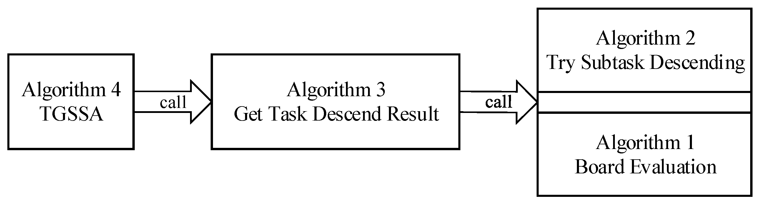
Algorithm 1 Board evaluation

Input: $board$, $numRowsRemoved$, $descendRow$, $pieceLen$; Output:  $score$;   1: $scor{e}_1=(descendRow+pieceLen/2)\times a_1$   2: $scor{e}_2=numRowsRemoved\times a_2$   3: $scor{e}_3=rowTransitions\left(board\right)\times a_3$   4: $scor{e}_4=columnTransitions\left(board\right)\times a_4$   5: $scor{e}_5=numberOfHoles\left(board\right)\times a_5$   6: $scor{e}_6=wellSum\left(board\right)\times a_6$   7: $score=scor{e}_1+scor{e}_2+scor{e}_3+scor{e}_4+scor{e}_5+scor{e}_6$   8: return  $score$

Algorithm 2 Try Subtask Descending

Input: $board$, $C_{i,j}$, $tStar{t}_{min}$, $column$, m; Output:  $board$, $numRowsRemoved$;   1: while  $tStar{t}_{min}+C_{i,j}<\left(rowofboard\right)$  do   2:    $board=\{board;\{0,0,\cdots ,0\left\}\right\}$ // add all-zero rows to $board$   3: end while   4: for all $k=1,2,\cdots ,C_{i,j}$ do   5:    $boar{d}_{tStar{t}_{min}+k,column}=1$   6: end if   7: $numRowsRemoved=\left(numberoffullrowsinboard\right)$   8: remove full rows in $board$   9: return [$board$, $numRowsRemoved$]

Algorithm 3 Get Task Descend Result

Input: $board$, $E_i$, $C_i$, m; Output:  $P_i$, $board$;   1: $tFinish=\{0,0,\cdots ,0\}$ // $|V_i|$ elements in total   2: $P_i=\{0,0,\cdots ,0\}$ // $|V_i|$ elements in total   3: for all j s.t. Ci,j ∈ Cj do   4:     $scor{e}_{max}=-\infty$   5:     $boar{d}_{new}=board$   6:     for all column = 1,2,⋯,m do   7:      $boar{d}_{temp}=board$   8:      $tStar{t}_{min}=(therowofthelast‘1’inboar{d}_{column})$   9:      for all k s.t. $e(V_{i,k},V_{i,j})\in E_i$ do  10:         $tStar{t}_{min}=max(tStar{t}_{min},tFinis{h}_k)$  11:      end for  12:      $[boar{d}_{temp},numRowsRemoved]=TrySubtaskDescending(boar{d}_{temp},C_{i,j},$ $tStar{t}_{min},column,m)$  13:      $score=BoardEvaluation(boar{d}_{temp},numRowsRemoved,tStar{t}_{min},C_{i,j},m)$  14:      if  $score>scor{e}_{max}$  then  15:           $scor{e}_{max}=score$  16:           $P_{i,j}=column$  17:           $boar{d}_{new}=boar{d}_{temp}$  18:      end if  19:     end for  20:     $board=boar{d}_{new}$  21: end for  22: return [$P_i$, $board$]

Algorithm 4 TGSSA

Input: $prioSeq$, $E=\{E_1,E_2,\cdots ,E_N\}$, $C=\{C_1,C_2,\cdots ,C_N\}$, m; Output: P   1: $P=\{P_1,P_2,\cdots ,P_N\}$   2: $board=\{0,0,\cdots ,0\}$ // initialized to be a $1\times m$ zero matrix   3: for all $i\in prioSeq$ do   4:     $[P_i,board]=GetTaskDescendResult(board,E_i,C_i,m)$   5: end for   6: return  P

5.1. Tetris Board Evaluation

Algorithm 1 is designed to evaluate a Tetris board, with higher scores indicating better alignment with optimization objectives.

Algorithm 1 accepts four inputs. The input $board$ corresponds to the Tetris board state after the latest piece placement and row removal. The input $numRowsRemoved$ specifies the number of rows cleared by the last piece placement. The $descendRow$ specifies the row index where the most recent piece landed, representing the height of the lowest row occupied by the piece after it has settled. The $pieceLen$ indicates the height of the most recently placed piece. The output, $score$, represents the evaluation score for the $board$, with higher values indicating a better alignment with the desired criteria. It should be noted that the $score$ is not necessarily a positive value.

Algorithm 1 evaluates a Tetris board based on six metrics. The score of each metric is weighted by a corresponding coefficient and is summed to obtain the final evaluation score.

• $scor{e}_1$ (line 1): $scor{e}_1$ represents the height of the center of gravity of the most recently placed piece, multiplied by the coefficient $a_1$. In the context of task scheduling, where pieces are $C_{i,j}\times 1$ strips, the center of gravity corresponds to the row index of the piece’s midpoint. Intuitively, we aim to place pieces as low as possible in Tetris. Therefore, $a_1$ is a negative value.
• $scor{e}_2$ (line 2): $scor{e}_2$ denotes the number of rows cleared as a result of placing the most recent piece, weighted by the coefficient $a_2$. Naturally, more clear rows is desirable. Thus, $a_2$ is positive.
• $scor{e}_3$ (line 3): $scor{e}_3$ represents the number of row transitions in the remaining Tetris board after the recently placed piece has landed and all completed rows have been cleared, weighted by $a_3$. A row transition occurs when a filled cell is adjacent to an empty cell or vice versa within a single row. The total number of row transitions is computed by summing this value of all rows. It is important to note that the calculation of row transitions in the task scheduling context differs from that in the standard Tetris game. In Tetris, the board is bounded by “walls” on both sides, which are typically modeled as columns of filled cells in the original El-Tetris algorithm. In the task scheduling scenario, however, each column represents a distinct processor (or core) and all processors access the same shared memory. Therefore, the leftmost and rightmost columns are treated as adjacent, forming a “cylindrical” structure. Since fewer row transitions are preferable, $a_3$ is a negative value.
• $scor{e}_4$ (line 4): $scor{e}_4$ measures the number of column transitions in the remaining Tetris board after the most recent piece placement and clearing completed rows, multiplied by $a_4$. A column transition occurs when a filled cell is adjacent to an empty cell or vice versa within a single column. Summing these transitions across all columns yields the total column transitions for the board. Similarly to row transitions, fewer column transitions are desirable, making $a_4$ a negative value.
• $scor{e}_5$ (line 5): $scor{e}_5$ represents the number of “holes” in the remaining Tetris board after the recent placement and removal of the completed rows. A “hole” in a column is defined as an empty cell that has at least one filled cell above it in the same column. The total number of holes is obtained by summing the holes in each column. Fewer holes are preferred, so $a_5$ is a negative value.
• $scor{e}_6$ (line 6): $scor{e}_6$ is the sum of “wells” in the remaining Tetris board after the most recent piece placement and row clear, weighted by $a_6$. A “well” is defined as an empty cell that lies over a column’s filled cells and is flanked by filled cells on both sides. The total number of wells is calculated as the number of such empty cells in the board. Similar to holes, fewer wells are desirable; therefore, $a_6$ is negative.

Among the six coefficients ($a_1$ to $a_6$), five are negative. As a result, the summation of $scor{e}_1$ to $scor{e}_6$, $score$, is likely to be a negative value. However, this does not pose an issue. In subsequent computations, the selection of the maximum score among the various $score$ remains unaffected.

5.2. Try Subtask Descending

Algorithm 2 primarily treats a given subtask as a Tetris piece and places it in a specified column within the Tetris board. Subsequently, it removes all completed rows.

Algorithm 2 accepts five inputs. The input $board$ represents the Tetris board before placing the subtask $V_{i,j}$. $C_{i,j}$ denotes the WCET of the subtask $V_{i,j}$. The $tStar{t}_{min}$ indicates the earliest possible start time for the execution of $V_{i,j}$. The $column$ specifies the target column where $V_{i,j}$ is to be placed, corresponding to the processor to which $V_{i,j}$ is assigned. The m is the total number of processors, equivalent to the total number of columns in the Tetris board, $board$. The output $numRowsRemoved$ of Algorithm 2 represents the number of rows cleared as a result of placing $V_{i,j}$. The output $board$ reflects the state of the Tetris board after placing $V_{i,j}$ and removing all cleared rows.

Placing the subtask $V_{i,j}$ involves marking the $C_{i,j}$ empty cells in the range from $tStar{t}_{min}+1$ to $tStar{t}_{min}+C_{i,j}$ as filled cells. To achieve this, the following steps are performed:

• Board expansion (line 1 to 3): If the number of rows in $board$ is less than $tStar{t}_{min}+C_{i,j}$, extend the board by adding rows until its number of rows equals $tStar{t}_{min}+C_{i,j}$.
• Filling cells (line 4 to 6): In the extended $board$, mark the $C_{i,j}$ empty cells in the n specified $column$, spanning form row $tStar{t}_{min}+1$ to $tStar{t}_{min}+C_{i,j}$, as filled cells.
• Row count recording (line 7): The number of completed rows in $board$ at this stage is recorded and denoted as $numRowsRemoved$.
• Row removal (line 8): Completed rows are removed from $board$.

5.3. Get Task Descend Result

For a given input DAG task, Algorithm 3 treats each of its subtasks as Tetris pieces and attempts to place them in each column of the Tetris board. For each subtask, Algorithm 3 identifies the column that yields the highest Tetris board score after placement, records the corresponding column, i.e., the processor to which the subtask is assigned, and updates the Tetris board accordingly.

Algorithm 3 accepts four inputs. The input $board$ represents the state of the Tetris board prior to the partitioning of the DAG task ${\tau }_i$. $E_i$ denotes the set of edges associated with the DAG task ${\tau }_i$. $C_i$ corresponds to the WCET of each subtask within ${\tau }_i$. m specifies the total number of processors, which is equivalent to the number of columns in the $board$. The output $P_i$ indicates the assignment of each subtask of ${\tau }_i$ to a specific processor.

The completion times $tFinish$ for the $|V_i|$ subtasks and the processor assignments $P_i$ for these $|V_i|$ subtasks are initialized. Subsequently, for each subtask $V_{i,j}$ in the task ${\tau }_i$, the following steps are executed sequentially.

• Initialization (lines 4 to 5): The maximum score $scor{e}_{max}$ for the subtask is set to be $-\infty$, and the current state of $board$ is stored in $boar{d}_{new}$.
• Processor assignment (lines 6 to 13): Through using Algorithm 2 $TrySubtaskDescending$, subtask $V_{i,j}$ is attempted to be assigned to each processor. For each attempt, a new temporary board $boar{d}_{temp}$ is generated. The state of the resulting board $boar{d}_{temp}$ can be evaluated through Algorithm 1$TetrisBoardEvaluation$ to obtain a score for the assignment.
• Score update (lines 14 to 18): If the score for the current processor assignment exceeds the current maximum score $scor{e}_{max}$, $scor{e}_{max}$ should be updated to the new score. The corresponding processor assignment should be recorded in $P_{i,j}$, and $boar{d}_{new}$ should be updated to the state of $boar{d}_{temp}$.
• Board update (line 20): After attempting to assign $V_{i,j}$ to all processors and determining the processor $P_{i,j}$ corresponding to the highest score, $board$ should be updated to $boar{d}_{new}$. This reflects the updated state of board after assigning $V_{i,j}$ based on the highest scoring placement.

Through this algorithm, each subtask $V_{i,j}$ is assigned to the processor that maximizes the overall board evaluation score, ensuring an optimized task allocation.

5.4. General Progress

After the layered construction of the aforementioned functions, the top-level algorithm becomes relatively straightforward, as shown in Algorithm 4.

The primary function of Algorithm 4 is to sequentially invoke Algorithm 3 on n DAG tasks based on their priority order.

Algorithm 4 accepts three inputs. $prioSeq$ represents the sequence of n DAG tasks sorted in descending order of priority, where $prioSe{q}_i$ denotes the index of the DAG task with the i-th highest priority. E represents the set of edges for all DAG tasks in the group. C is the WCET matrix for all DAG tasks. The output of Algorithm 4 is a single variable, P, which contains the processor assignments for each subtask of every DAG task. Specifically, P consists of n elements, where each element $P_i$ is an array of v elements. The j-th element of $P_i$ indicates the processor to which the j-th subtask of the i-th DAG task has been assigned.

At the beginning of Algorithm 4, two variables, P and $board$, are initialized. P is the final output of the function, as defined earlier. Initially, P consists of n elements, where each element is an array of $|V_i|$ zeros. The specific initialization value (e.g., zeros) is not critical. It can be any value of your choice. The purpose of this step is simply to preallocate memory for the P matrix during program execution. $board$ represents the Tetris board used to simulate the Tetris game. The board has m columns (corresponding to the number of processors) and is initially a single row. Each element in this row is initialized to zero, indicating that no blocks have yet been placed on the board.

The algorithm iterates n times; there, in each iteration, a DAG task index i is sequentially extracted from $prioSeq$ and passed to Algorithm 3 $GetTaskDescendResult$. Each iteration of Algorithm 3 serves two primary purposes. They are partitioning the subtask of $|V_i|$ with the resulting assignments stored in $P_i$, and updating the current state of the Tetris board. Finally, after completing N iterations, the P matrix is returned as the output.

In Algorithm 1, the computational complexity of the calculation of $scor{e}_1$ is $O\left(1\right)$. The calculation of each parameter from $scor{e}_2$ to $scor{e}_6$ traverses the Tetris board at most once. The Tetris board has m columns. In the worst case, it has $|V_i| \times {max}_j\left(C_{i,j}\right)$ rows, where ${max}_j\left(C_{i,j}\right)$ is a constant. The computational complexity of Algorithm 1 is $O\left(m\right|V_i\left|\right)$. Lines 1 to 6 of Algorithm 2 traverse the Tetris board less than once, and lines 7 to 8 traverse it at most once. The computational complexity of Algorithm 2 is $O\left(m\right|V_i\left|\right)$. The “for” loops in line 3 and line 6 of Algorithm 3 need to execute Algorithm 1 and Algorithm 2 $m|V_i|$ times, respectively, making the computational complexity of Algorithm 3 $O\left(m^2\right|V_i{|}^2)$. Algorithm 4 executes Algorithm 3 N times. Therefore, the computational complexity of it is $O\left(N{m}^2\right|V_i{|}^2)$, i.e., the computational complexity of TGSSA is $O\left(N{m}^2\right|V_i{|}^2)$.

5.5. Discussion

As mentioned before, this model needs to use different weight coefficients in different scenarios, but we have not yet found a low-computational-complexity and efficient way to characterize the relationship between the coefficients and specific scenarios. Therefore, these weight coefficients need to be calculated before using them in specific scenarios. In future work, it is possible to explore a low-computational-complexity and efficient way to characterize the relationship between the coefficients and specific scenarios, and incorporate it into the current model to improve the model.

6. Experiments

In this section, the performance of the TGSSA is evaluated by comparing it with two other scheduling strategies. They are random allocation and the Equilibrium Remaining Utilization (ERU) algorithm, which are used in the latest state-of-the-art scheduling strategy [12].

The generation of tested DAG sets and actual platform settings are introduced before presenting the performance evaluation. DAG set generation includes the chosen parameters and the generation progress of DAG sets. The evaluation of performance is divided into two parts. One part is the schedulability test through WCRT analysis, and the other part is executing allocated tasks on an actual real-time platform.

6.1. Tested DAG Sets Generation

To make the experimental results more general, we strive to maintain consistency with previous studies regarding DAG parameters and DAG generation tools. We control the generation of DAG task sets using the following five DAG parameters [13]:

• U: The utilization of the DAG task set $\Gamma$.
• N: The number of DAG tasks in $\Gamma$.
• $|V_i|$: The number of subtasks in ${\tau }_i$
• p: The probability of creating edges.
• m: The number of processors.

The generation of each DAG task ${\tau }_i$ involves two primary steps, topological structure generation and WCET assignment. In the topological structure generation step, the topological structure of the DAG task is created using the $GenerateG\left(\right|V_i|,p)$ method described in [24]. In the WCET assignment step, a set of $|V_i|$ random integers is drawn from the interval $[1,100]$ as the WCET values $C_{i,j}$ for each subtask in the DAG task. The overall WCET of the DAG task, $Csu{m}_i$, can be calculated as $Csu{m}_i={\sum }_{j=1}^{|V_i|}{C}_{i,j}$. This process is repeated N times to generate the topological structures and WCET values for N distinct DAG tasks.

To determine the utilization $U_i$ for each task ${\tau }_i$ in a given task set $\Gamma$ with a total utilization U, we employ the $Randfixedsum$ algorithm. This algorithm generates a matrix where the sum of the elements is fixed, while allowing the user to specify the maximum and minimum values for each element. By using this method, we ensure that the utilization $U_i$ of any individual task ${\tau }_i$ does not exceed 1. Next, the period $T_i$ of each DAG task can be calculated using the equation $T_i=Csu{m}_i/U_i$. Fixed priorities ${\pi }_i$ are assigned to each DAG task in $\Gamma$ based on their relative periods, following the RMS policy. Finally, the generated DAG task set $\Gamma$ is input into the respective algorithms to assign subtasks to processors. At this point, the task set $\Gamma$ is ready for further WCRT analysis or testing on a real platform.

To demonstrate the consistency between simulation results and actual platform performance, both the WCRT analysis and actual platform tests presented in this section are conducted using a similar dataset [25,26]. The generated test dataset adopts the following default parameters: $U=2.0$, $N=20$, $|V_i|=20$, $p=10\%$, and $m=16$. Under these default settings, we vary one parameter at a time while keeping the others fixed to generate additional datasets.

• U: 1.0, 1.2, 1.4, 1.6, 1.8, 2.0, 2.2.
• N: 20, 25, 30, 35, 40, 45, 50.
• $|V_i|$: 10, 14, 18, 22, 26, 30.
• p: 5%, 10%, 15%, 20%, 25%, 30%.
• m: 2, 4, 8, 16.

Hence, the total utilization of a task set $\Gamma$ will be set from 1 to 2.2 with each step increment of 0.2. The number of DAG tasks in a task set will be set from 20 to 50 with each step increment of 5. The number of subtasks in a DAG task will be set from 10 to 30 with each step increment of 4. The number of processors will be set to be 2, 4, 8, and 16 [26]. The topological matrix of the DAG task is generated by a DAG generation tool with $GenerateG\left(\right|V_i|,p)$, and p will be set from 5% to 30% with each step increment of 5% [24].

We use one DAG parameter as a variable each time and fix the remaining four DAG parameters and test with five DAG parameters sequentially as variables to verify our algorithm performance in various scenarios. We separately generate one thousand DAG task sets for each varied parameter. We define the percentage of schedulable task sets under a given m as acceptance ratio. For instance, the acceptance ratio is 13 percent under $m=16$, which represents that 130 task sets are schedulable. For average WCRT and acceptance ratio, we only count data from schedulable task sets.

It is important to note that when using TGSSA for task partitioning, the coefficients of Algorithm 1 are adjusted to account for their varying sensitivity to different parameter changes. Specifically, when U, N, or m are the variables, the coefficients are set as follows: $a1=-4.5$, $a2=3.4$, $a3=-3.2$, $a4=-9.3$, $a5=-9$, $a6=-5.5$. When $|V_i|$ and p are variables, the coefficients are adjusted to $a1=-4.5$, $a2=3.4$, $a3=-4$, $a4=-8$, $a5=-11$, $a6=-6$.

6.2. Actual Platform Settings

The actual testing platform is a laptop equipped with an AMD Ryzen 7 4800U processor designed by Advanced Micro Devices company in California, United States featuring 8 cores and 16 threads, along with 16 GB of DDR4 3200 MHz memory. The system runs Ubuntu 22.04 with an RT-Patched Linux kernel [27]. The specific patch version applied is patch-6.5.2-rt8.

It is worth mentioning that before compiling the patched kernel, the following configurations should be made in make menuconfig command:

• In General setup -> Preemption Model, select Fully Preemptible Kernel (RT).
• Uncheck Device Drivers -> Staging drivers.
• In General setup -> Timer subsystem, enable High Resolution Timer Support.
• In processor type and features -> Timer frequency, set the frequency to 1000 Hz.

After saving and exiting the configuration interface, modify the generated .config file. Specifically, leaving the double quotes themselves intact, remove the content inside the double quotes in the line CONFIG_SYSTEM_TRUSTED_KEYS=‘‘’’.

After compiling the RT-Patched kernel and setting it as the default kernel for the system, restart the computer. To verify the kernel version, use the uname -a command. The output should display Linux … 6.5.2-rt8 #2 SMP PREEMPT_RT … x86_64 GNU/Linux.

To run tasks and subtasks on actual platform, we used the pthread.h library in C language. Each subtask is created using function pthread_create(), the relationship between subtasks is limited using function pthread_cond_wait(), and the execution time of each subtask is limited using sys/time.h. The threads generated in this way are consistent with the actual threads.

6.3. Experiment Results

As mentioned at the beginning of this section, the performance evaluation in this article consists of a schedulability test through WCRT analysis and executing allocated tasks on an actual real-time platform.

Due to the limitations of existing WCRT analysis algorithms, the schedulability rates derived from their analysis are typically much lower than those observed in real platform tests. In the real platform tests conducted in this article, under all selected test conditions, the schedulability rates for all algorithms were consistently above 90%, with no significant performance differences between the algorithms. As such, further details are omitted. The only exception occurs when the number of processors is set to 2, where the schedulability rate for the random allocation algorithm falls below 30%.

Figure 3 shows the average WCRT drawn from WCRT analysis. A lower average WCRT indicates better performance. In almost all cases, TGSSA achieves a lower average WCRT compared to both random allocation and ERU. Figure 4 shows the schedulability ratio drawn from WCRT analysis. It is clear that TGSSA achieves a higher schedulability ratio compared to both random allocation and ERU in almost all cases. Figure 5 shows the average WCRT on the actual real-time platform. The trends presented in Figure 3 and Figure 5 are generally consistent. Next, we will focus on analyzing the data in Figure 5.

Figure 5a illustrates the average WCRT of the DAG task set as the utilization varies. From the figure, it is evident that for the same utilization values, the average WCRT obtained using TGSSA is lower compared to both the random and ERU algorithms. Specifically, for utilization values $U=1.0,1.2,1.4,1.6,1.8,2.0,2.2$, the WCRT improves over random by 34.54%, 36.05%, 32.41%, 31.20%, 31.99%, 31.29%, and 25.24%, respectively, and improves over ERU by 11.48%, 15.33%, 5.76%, 5.54%, 6.32%, 3.78%, and 3.03%, respectively.

Figure 5b presents the average WCRT of the DAG task set as the number of tasks varies. From the figure, it is clear that for the same number of tasks, the average WCRT obtained using TGSSA is lower than that of both the random and ERU algorithms. Specifically, for $N=20,25,30,35,40,45,50$, the WCRT is improved over random by 29.31%, 40.04%, 33.60%, 37.07%, 41.43%, 41.50%, and 44.86%, respectively, and improved over ERU by 3.74%, 12.21%, 5.94%, 14.37%, 10.67%, 11.97%, and 16.68%, respectively.

Figure 5c shows the average WCRT of the DAG task set as the number of subtasks varies. From the figure, it can be observed that for the same number of subtasks, the average WCRT achieved by TGSSA is lower than that of the random algorithm, and in cases where $|V_i|$ is higher, it is also lower than that of ERU. Specifically, for $|V_i|=10,14,18,22,26,30$, the WCRT improves over random by 25.59%, 26.70%, 32.18%, 29.61%, 24.77%, and 26.30%, respectively, and improves over ERU by −3.01%, −1.40%, 4.19%, 5.02%, 3.20%, and 5.58%, respectively.

It can be observed that when $|V_i|$ is relatively low, the performance of TGSSA is suboptimal. This is due to the use of a fixed set of weight values in the scoring algorithm; meanwhile, the ratio of subtask quantity to processor quantity changes too much. Fixed weights may not be suitable for all scenarios. Taking the scenario where $|V_i|$ is variable as an example, when $|V_i|$ is low, the impact of certain factors is weaker, suggesting that the weight coefficients should be appropriately adjusted to better accommodate such conditions.

Figure 5d illustrates the average WCRT of the DAG task set as the probability of creating edges varies. From the figure, it is evident that for the same probability of creating edges, TGSSA achieves a lower average WCRT than both the random and ERU algorithms in most cases. Specifically, for $p=5,10,15,20,25,30$, the WCRT improves over random by 42.27%, 28.43%, 18.42%, 14.75%, 16.95%, and 12.28%, respectively, and improves over ERU by 8.46%, 6.54%, 2.86%, −0.76%, 4.16%, and 3.26%, respectively.

Figure 5e presents the average WCRT of the DAG task set as the number of processors varies. Due to the significant variation in average WCRT with respect to the number of processors (with random values of 163604.4, 38565.0, 21032.7, and 15370.7), the plotting method was adjusted. Unlike the previous figures, which used absolute values, this figure uses relative values, representing the ratio of WCRT for each algorithm to that of the random algorithm. From the figure, it is apparent that for the same number of processors, TGSSA achieves a lower average WCRT than random, and in higher values of m, it also outperforms ERU. Specifically, for $m=2,4,6,8$, the WCRT improves over random by 33.82%, 35.41%, 31.06%, and 32.30%, respectively, and over ERU by −3.38%, 4.97%, 2.40%, and 7.25%, respectively. Overall, TGSSA has achieved excellent scheduling performance.

7. Conclusions and Future Work

This article draws inspiration from the Tetris algorithm (El Tetris) and proposes a new scheduling algorithm with multiple-heuristic parameters. We simulated the real-time DAG task scheduling process as a Tetris game process and completed the scheduling on multiple processors. Compared with previous algorithms, TGSSA achieved better average WCRT analysis results, processor utilization, real-time system stability, and average WCRT observed in an actual RTOS.

In our future work, we plan to address the following issues. The first question is determining how to optimize coefficients for multiple-heuristic parameters through artificial intelligence methods to achieve better scheduling results [28]. The second issue is establishing an effective task clustering strategy to reduce algorithmic complexity, especially for large DAG with intricate parallel dependencies. Finally, we aim to adapt our algorithm for efficient real-time performance as an online scheduling solution combining with compute-bound parallel jobs and I/O-bound parallel jobs in multiprocessor systems [29].

References

1. Hiroyuki, C. RT-Seed: Real-Time Middleware for Semi-Fixed-Priority Scheduling. In Proceedings of the 2016 IEEE 19th International Symposium on Real-Time Distributed Computing (ISORC), York, UK, 17–20 May 2016; pp. 124–133. [Google Scholar]
2. Ranvijay; Yadav, R.S.; Smriti, A. Efficient energy constrained scheduling approach for dynamic real time system. In Proceedings of the 2010 First International Conference On Parallel, Distributed and Grid Computing (PDGC 2010), Solan, India, 28–30 October 2010; pp. 284–289. [Google Scholar]
3. Biao, H.; Cao, Z.C.; Zhou, M.C. Scheduling Real-Time Parallel Applications in Cloud to Minimize Energy Consumption. IEEE Trans. Cloud Comput. 2022, 10, 662–674. [Google Scholar]
4. Hu, M.L.; Bharadwaj, V. Dynamic Scheduling of Hybrid Real-Time Tasks on Clusters. IEEE Trans. Comput. 2014, 63, 2988–2997. [Google Scholar] [CrossRef]
5. Dong, W.; Chen, C.; Liu, X.; Zheng, K.G.; Chu, R.; Bu, J.J. FIT: A Flexible, Lightweight, and Real-Time Scheduling System for Wireless Sensor Platforms. IEEE Trans. Parallel Distrib. Syst. 2010, 21, 126–138. [Google Scholar] [CrossRef]
6. Zhu, Q.; Zeng, H.B.; Zheng, W.; Marco Di, N.; Alberto, S.V. Optimization of task allocation and priority assignment in hard real-time distributed systems. ACM Trans. Embed. Comput. Syst. (TECS) 2012, 11, 85–96. [Google Scholar] [CrossRef]
7. Alessandro, B.; Giorgio, B. Engine control: Task modeling and analysis. In Proceedings of the 2015 Design, Automation & Test in Europe Conference & Exhibition (DATE), Grenoble, France, 9–13 March 2015; pp. 525–530. [Google Scholar]
8. Nong, G.; Hamdi, M. On the provision of quality-of-service guarantees for input queued switches. IEEE Commun. Mag. 2000, 38, 62–69. [Google Scholar]
9. Biondi, A.; Di Natale, M.; Buttazzo, G. Response-Time Analysis of Engine Control Applications Under Fixed-Priority Scheduling. IEEE Trans. Comput. 2018, 67, 687–703. [Google Scholar] [CrossRef]
10. Alessandro, B.; Alessandra, M.; Mauro, M.; Marco, D.N.; Giorgio, B. Exact Interference of Adaptive Variable-Rate Tasks under Fixed-Priority Scheduling. In Proceedings of the 2014 26th Euromicro Conference on Real-Time Systems, Madrid, Spain, 8–11 July 2014; pp. 165–174. [Google Scholar]
11. Chen, Y.M.; Liu, S.L.; Chen, Y.J.; Ling, X. A scheduling algorithm for heterogeneous computing systems by edge cover queue. Knowl.-Based Syst. 2023, 265, 110369. [Google Scholar] [CrossRef]
12. Wu, Y.L.; Zhang, W.Z.; Guan, N.; Ma, Y.H. TDTA: Topology-Based Real-Time DAG Task Allocation on Identical Multiprocessor Platforms. IEEE Trans. Parallel Distrib. Syst. 2023, 34, 2895–2909. [Google Scholar] [CrossRef]
13. Wu, Y.L.; Zhang, W.Z.; Guan, N.; Tang, Y. Improving Interference Analysis for Real-Time DAG Tasks Under Partitioned Scheduling. IEEE Trans. Comput. 2022, 71, 1495–1506. [Google Scholar] [CrossRef]
14. Abusayeed, S.; Kunal, A.; Lu, C.Y.; Christopher, G. Multicore Real-Time Scheduling for Generalized Parallel Task Models. In Proceedings of the 2011 IEEE 32nd Real-Time Systems Symposium, Washington, DC, USA, 29 November–2 December 2011; Volume 10, pp. 217–226. [Google Scholar]
15. Marko, B.; Sanjoy, B. Limited Preemption EDF Scheduling of Sporadic Task Systems. IEEE Trans. Ind. Inform. 2010, 6, 579–591. [Google Scholar]
16. Shinpei, K.; Yutaka, I. Gang EDF Scheduling of Parallel Task Systems. In Proceedings of the 2009 30th IEEE Real-Time Systems Symposium, Washington, DC, USA, 1–4 December 2009; pp. 459–468. [Google Scholar]
17. Karthik, L.; Shinpei, K.; Ragunathan, R. Scheduling Parallel Real-Time Tasks on multicore Processors. In Proceedings of the 2010 31st IEEE Real-Time Systems Symposium, San Diego, CA, USA, 30 November–3 December 2010; pp. 259–268. [Google Scholar]
18. Daniel, C.; Alessandro, B.; Geoffrey, N.; Giorgio, B. Partitioned Fixed-Priority Scheduling of Parallel Tasks Without Preemptions. In Proceedings of the 2018 IEEE Real-Time Systems Symposium (RTSS), Nashville, TN, USA, 11–14 December 2018; pp. 421–433. [Google Scholar]
19. Özkaya, M.Y.; Benoit, A.; Uçar, B.; Herrmann, J.; Çatalyürek, Ü.V. A Scalable Clustering-Based Task Scheduler for Homogeneous Processors Using DAG Partitioning. In Proceedings of the 2019 IEEE International Parallel and Distributed Processing Symposium (IPDPS), Rio de Janeiro, Brazil, 20–24 May 2019; pp. 155–165. [Google Scholar]
20. El-Tetris: An Improvement on Pierre Dellacheries Algorithm. Available online: https://imake.ninja/el-tetris-an-improvement-on-pierre-dellacheries-algorithm/ (accessed on 26 December 2024).
21. Abusayeed, S.; David, F.; Li, J.; Kunal, A.; Lu, C.Y.; Christopher, D.G. Parallel Real-Time Scheduling of DAGs. IEEE Trans. Parallel Distrib. Syst. 2014, 25, 3242–3252. [Google Scholar]
22. Shamit, B.; Zhao, Y.C.; Zeng, H.B.; Yang, K.H. Optimal Implementation of Simulink Models on Multicore Architectures with Partitioned Fixed Priority Scheduling. In Proceedings of the 2018 IEEE Real-Time Systems Symposium (RTSS), Nashville, TN, USA, 11–14 December 2018; Volume 10, pp. 242–253. [Google Scholar]
23. Jose, F.; Geoffrey, N.; Vincent, N.; Luís Miguel, P. Response time analysis of sporadic DAG tasks under partitioned scheduling. In Proceedings of the 2016 11th IEEE Symposium on Industrial Embedded Systems (SIES), Krakow, Poland, 23–25 May 2016; pp. 1–10. [Google Scholar]
24. Erdős, P.; Alfréd, R. On Random Graphs I. Publ. Math. 1959, 4, 3286–3291. [Google Scholar] [CrossRef]
25. Davis, R.I.; Burns, A. Response Time Upper Bounds for Fixed Priority Real-Time Systems. In Proceedings of the 2008 Real-Time Systems Symposium, Washington, DC, USA, 30 November–3 December 2008; pp. 407–418. [Google Scholar]
26. Guan, N.; Martin, S.; Yi, W.; Yu, G. New Response Time Bounds for Fixed Priority Multiprocessor Scheduling. In Proceedings of the 2009 30th IEEE Real-Time Systems Symposium, Washington, DC, USA, 1–4 December 2009; pp. 387–397. [Google Scholar]
27. RT-Linux System. Available online: https://en.wikipedia.org/wiki/RTLinux (accessed on 26 December 2024).
28. Anderson, G.G. Application of Standard Optimization Methods to Operating System Scheduler Tuning. In Operating System Scheduling Optimization; University of Johannesburg: Johannesburg, South Africa, 2013; pp. 56–69. [Google Scholar]
29. Wiseman, Y.; Feitelson, D.G. Paired gang scheduling. IEEE Trans. Parallel Distrib. Syst. 2003, 14, 581–592. [Google Scholar] [CrossRef]
Figure 1. An example of a DAG task τ i with eight subtasks and C s u m i = 95 , T i = D i = 100 . A dummy exit subtask will be added to the graph as a child subtask of V i , 3 , V i , 7 , and V i , 8 .
Electronics 14 00098 g001
Figure 2. The relationship between algorithms.
Electronics 14 00098 g002
Figure 3. Average WCRT from WCRT analysis algorithm (RTA). (a) Average WCRT with changing utilization. (b) Average WCRT with changing number of tasks. (c) Average WCRT with changing number of subtasks. (d) Average WCRT with varied probability of creating edges. (e) Average WCRT with changing number of processors.
Electronics 14 00098 g003
Figure 4. Schedulability ratio from WCRT analysis algorithm (RTA). (a) Schedulable ratio with changing utilization. (b) Schedulable ratio with changing number of tasks. (c) Schedulable ratio with changing number of subtasks. (d) Schedulable ratio with varied probability of creating edges. (e) Schedulable ratio with changing number of processors.
Electronics 14 00098 g004
Figure 5. Average WCRT on actual real-time platform. (a) Average WCRT with changing utilization. (b) Average WCRT with changing number of tasks. (c) Average WCRT with changing number of subtasks. (d) Average WCRT with varied probability of creating edges. (e) Average WCRT with changing number of processors.
Electronics 14 00098 g005
Disclaimer/Publisher’s Note: The statements, opinions and data contained in all publications are solely those of the individual author(s) and contributor(s) and not of MDPI and/or the editor(s). MDPI and/or the editor(s) disclaim responsibility for any injury to people or property resulting from any ideas, methods, instructions or products referred to in the content.