Research on Frequency Discrimination Method Using Multiplicative-Integral and Linear Transformation Network

Abstract

In this paper, a frequency discrimination method using a multiplicative-integral and linear transformation network is proposed. In this method, two preset differential frequency signals and frequency modulation signals are transformed by multiplication and integration, and then the instantaneous frequency parameters of the frequency modulation signal are accurately analyzed by the linear transformation network to restore the original modulation signal. Compared with the phase discriminator, the simulation results show that this method has a higher frequency discrimination bandwidth. In addition, this method has better anti-noise performance, and the frequency discrimination distortion caused by noise with a different Signal-to-Noise Ratio is reduced by 33.80% on average compared with the phase discriminator. What is more, the carrier center frequency error has little influence on the frequency discrimination quality of this method, which solves the problem that most common frequency discriminators are seriously affected by the carrier center frequency error. This method requires a low accuracy of carrier center frequency, which makes it extremely suitable for digital frequency discrimination technology and can meet the needs of various frequency discrimination occasions.

1. Introduction

Frequency modulation (FM) and frequency discrimination technology is one of the important technologies in modern radio communication, which is widely used in various applications, such as communication, mapping, navigation, and national defense [1]. Frequency discrimination is the process of reproducing modulation signals from FM signals. Over the years, frequency discriminators [2] have played important roles in the stabilization of oscillators and in the demodulation of angular modulated signals [3]. Slope discriminator, phase discriminator (PD) and pulse digital discriminator are commonly used in common frequency discrimination methods. The selection of the frequency discrimination method mainly depends on the relative frequency offset requirements of the FM signal and the characteristics of the frequency discriminator. In general, FM signals have a very small relative frequency offset and usually complete frequency discrimination with a slope frequency discriminator or phase discriminator. The slope discriminator is mainly composed of a frequency modulation to amplitude modulation (AM) converter and envelope detector. Its core is the FM-AM conversion of the FM signal by using the amplitude–frequency characteristics of the detuned loop. The amplitude–frequency characteristic curve [4] near the center frequency of the detuned loop is linear, and the frequency change of the input FM signal can be linearly converted into the proportional amplitude change so that the output signal can be converted into the AM signal. Then, the envelope signal on the AM signal can be detected by the envelope detector, which is the original modulation signal. Due to the narrow linear range of the amplitude–frequency characteristics of the FM-AM converter and the nonlinear characteristics of the envelope detector, the slope frequency discriminator has the problems of a narrow discrimination frequency band and large distortion.

The phase discriminator is mainly composed of a frequency-phase converter and a phase detector. The frequency phase converter converts the frequency change of the FM signal into a phase change through the RLC phase shift network. The phase detector [5,6,7] is used to detect the phase shift of the signal. The detection result of the phase detector is a sine function of the phase shift, which has good linearity only when the phase shift is less than 30 ° and can restore the original modulation signal in equal proportion, so the frequency discrimination bandwidth of the phase frequency detector is very limited. The above common frequency discrimination methods need accurate carrier center frequency parameters to have better frequency discrimination characteristics. In other words, the limitation of phase noise [8] on microwave communication and the impact of Doppler effect [9], or the central frequency deviation caused by transmitter performance, will greatly affect the quality of the frequency discrimination.

To reduce the limitation of the central frequency deviation caused by various external factors on the frequency discrimination performance and improve the quality of frequency discrimination, this study proposes a frequency discrimination method using multiplicative-integral and linear transformation network (abbreviated as MIFD). The FM signal is sent to the multiplicative-integral transformation network to transform with two preset differential frequency signals, respectively. The real-time frequency parameters of the FM signal can be analyzed by linear processing. The angular frequency of the actual FM signal includes the carrier center frequency and the frequency offset caused by the modulation, which is linear with the original modulation signal. The amplitude information of the original modulation signal can be analyzed by sending the result of the multiplicative-integral transformation to the linear transformation network. Starting from the theoretical basis of FM signal, this paper describes the theoretical derivation process of the proposed method and proves its reliability. The proposed frequency discrimination method is simulated in MATLAB to verify its frequency discrimination capability and characteristics. By comparing with the frequency discrimination results of the common product phase discriminator, this paper analyzes its advantages and solves the problem of carrier center frequency deviation of the common frequency discrimination methods. In addition, this method has wider frequency discrimination bandwidth, smaller frequency discrimination distortion, and better anti-noise performance.

2. Theory

The carrier signal is $u_c\left(t\right)=U_{cm}cos{\omega }_{c}t$, where $U_{cm}$ is the carrier amplitude, and ${\omega }_c$ is the carrier angular frequency. The modulation signal is $u_{\Omega }\left(t\right)=U_{\Omega m}cos\Omega t$, where $U_{\Omega m}$ is the amplitude of the modulation signal, and $\Omega$ is the angular frequency of the modulation signal. The FM signal is obtained by frequency modulating the modulating signal and the carrier signal. The instantaneous angular frequency of the FM signal will change according to the law of $u_{\Omega }\left(t\right)$ based on ${\omega }_c$. The instantaneous angular frequency can be expressed as:

$$\begin{array}{cc}\hfill \omega \left(t\right)& ={\omega }_c+k_f{u}_{\Omega }\left(t\right)\hfill \\ \hfill & ={\omega }_c+k_f{U}_{\Omega m}cos\Omega t\hfill \\ \hfill & ={\omega }_c+\Delta {\omega }_{m}cos\Omega t\hfill \\ \hfill & ={\omega }_c+\Delta \omega \left(t\right)\hfill \end{array}$$

(1)

where $k_f$ is the sensitivity of the modulator, $\Delta \omega \left(t\right)=k_f{U}_{\Omega m}cos\Omega t$ is the instantaneous angular frequency offset of the FM signal, and $\Delta {\omega }_m=k_f{U}_{\Omega m}$ is the maximum angular frequency offset of FM signal. Similarly, the instantaneous frequency of the FM signal will change based on the central frequency of the carrier according to the law of $u_{\Omega }\left(t\right)$, and the instantaneous frequency can be expressed as:

$$\begin{array}{cc}\hfill f\left(t\right)& =f_c+\Delta f\left(t\right)\hfill \\ \hfill & =f_c+\frac{\Delta \omega \left(t\right)}{2\pi }\hfill \\ \hfill & =f_c+\frac{k_f{U}_{\Omega m}cos\Omega t}{2\pi }\hfill \\ \hfill & =f_c+\Delta f_{m}cos\Omega t\hfill \end{array}$$

(2)

where $\Delta f\left(t\right)=\frac{k_f{U}_{\Omega m}cos\Omega t}{2\pi }$ is the instantaneous frequency offset of the FM signal, and $\Delta f_m=\frac{k_f{U}_{\Omega m}}{2\pi }$ is the maximum frequency offset of the FM signal. According to Equations (1) and (2), the modulation signal can be recovered by accurately analyzing the instantaneous angular frequency or instantaneous frequency of the FM signal.

The phase change caused by the input modulation signal is usually used to represent the FM signal when analyzing it. According to Equation (1), the instantaneous phase change of the FM signal is $\Delta \phi \left(t\right)={\int }_0^t\Delta \omega \left(t\right)\mathrm{d}t=k_f{\int }_0^t{u}_{\Omega }\left(t\right)\mathrm{d}t$. Assuming that the initial phase of FM signal is zero, the formula for expressing the FM signal [10] with phase change caused by modulation signal is:

$$\begin{array}{cc}\hfill u_{FM}\left(t\right)& =U_{cm}cos\left({\omega }_{c}t+k_f{\int }_0^t{u}_{\Omega }\left(t\right)\mathrm{d}t\right)\hfill \\ \hfill & =U_{cm}cos\left({\omega }_{c}t+k_f{U}_{\Omega m}{\int }_0^{t}cos\Omega t\mathrm{d}t\right)\hfill \\ \hfill & =U_{cm}cos\left({\omega }_{c}t+\frac{\Delta {\omega }_{m}sin\Omega t}{\Omega }\right)\hfill \\ \hfill & =U_{cm}cos\left({\omega }_{c}t+\frac{\Delta f_{m}sin\Omega t}{f_t}\right)\hfill \\ \hfill & =U_{cm}cos({\omega }_{c}t+m_{f}sin\Omega t)\hfill \end{array}$$

(3)

where $f_t$ is the frequency of the modulation signal. $m_f=\frac{\Delta {\omega }_m}{\Omega }=\frac{\Delta f_m}{f_t}$ is the FM index, which represents the maximum additional phase of the FM signal. According to Equation (2), under the condition of certain FM index $m_f$, the modulation signal of the unit amplitude obtained through the instantaneous frequency analysis of FM signal can be expressed as:

$$\begin{array}{c}\hfill cos\Omega t=\frac{[f\left(t\right)-f_c]}{m_f{f}_t}\end{array}$$

(4)

Figure 1 shows the system model of frequency discrimination method using a multiplicative-integral and linear transformation network. The system is composed of a multiplicative-integral transformation network and linear transformation network. $u_i\left(t\right)$ is the input FM signal, and $u_{s1}\left(t\right)$ and $u_{s2}\left(t\right)$ are the preset differential frequency signals. The input FM signal and two preset differential frequency signals complete the multiplicative-integral transformation, respectively. Then, the instantaneous frequency of FM signal is analyzed and the modulation signal $u_o\left(t\right)$ can be restored through linear transformation to complete the frequency discrimination.

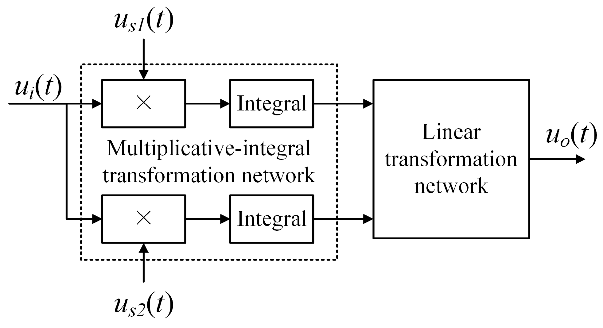
2.1. Multiplicative-Integral Transformation Network

The frequency of two differential frequency signals is $f_1$ and $f_2$. They should be close to the carrier frequency and have an appropriate maximum common divisor $f_0(f_0<f_c)$, so $f_1=n_1{f}_0$, $f_2=n_2{f}_0$, where $n_1$ and $n_2$ are positive integers and satisfy $n_1\ne n_2$.

Let $\tau =f_{0}t$, then the differential frequency signal $u_{s1}\left(t\right)$ can be expressed as:

$$\begin{array}{c}\hfill u_{s1}\left(\tau \right)=sin2\pi n_1\tau =\frac{e^{j2\pi n_1\tau }-e^{-2j\pi n_1\tau }}{2j}\end{array}$$

(5)

The differential frequency signal $u_{s2}\left(t\right)$ can be expressed as:

$$\begin{array}{c}\hfill u_{s2}\left(\tau \right)=sin2\pi n_2\tau =\frac{e^{j2\pi n_2\tau }-e^{-2j\pi n_2\tau }}{2j}\end{array}$$

(6)

The FM signal can be expressed as:

$$\begin{array}{cc}\hfill u_i\left(\tau \right)& =U_{cm}cos(2\pi x\tau +\phi )\hfill \\ \hfill & =\frac{e^{j2\pi x\tau +j\phi }+e^{-j2\pi x\tau -j\phi }}{2}\hfill \end{array}$$

(7)

where $\phi$ is the initial phase of the FM signal when it is sent into the multiplicative-integral transformation network. The multiplying parameter of the instantaneous frequency $f\left(t\right)$ of FM signal and $f_0$ is a positive real number expressed as:

$$\begin{array}{c}\hfill x\left(t\right)=\frac{f\left(t\right)}{f_0}\end{array}$$

(8)

In the process of multiplicative-integral transformation, the period corresponding to the frequency $f_0$ is taken as the integration time, so the integration time for $\tau$ is 0 to ${\tau }_0$, where ${\tau }_0=f_0{T}_0=1$. The conversion process of the FM signal and differential frequency signal $u_{s1}\left(t\right)$ is shown in Equation (9). The conversion process of the FM signal and differential frequency signal $u_{s2}\left(t\right)$ is shown in Equation (10):

$$\begin{array}{cc}\hfill Q_1& ={\int }_0^1{u}_i\left(\tau \right)u_{s1}\left(\tau \right)\mathrm{d}\tau \hfill \\ \hfill & =U_{cm}{\int }_0^1\frac{e^{j\left(2\pi x\tau \right)}+e^{-j\left(2\pi x\tau \right)}}{2}\frac{e^{j2\pi n_1\tau }-e^{-j2\pi n_1\tau }}{2j}\mathrm{d}\tau \hfill \\ \hfill & =\frac{U_{cm}}{4j}\left\{\frac{e^{j[2\pi (x+n_1)\tau +\phi ]}}{j2\pi (x+n_1)}{|}_0^1-\frac{e^{j[2\pi (x-n_1)\tau +\phi ]}}{j2\pi (x-n_1)}{|}_0^1\right\}+\frac{U_{cm}}{4j}\left\{-\frac{e^{-j[2\pi (x-n_1)\tau +\phi ]}}{j2\pi (x-n_1)}{|}_0^1+\frac{e^{-j[2\pi (x+n_1)\tau +\phi ]}}{j2\pi (x+n_1)}{|}_0^1\right\}\hfill \\ \hfill & =\frac{U_{cm}}{2\pi }\left[\frac{e^{j(2\pi x+\phi )}+e^{-j(2\pi x+\phi )}-(e^{j\phi }+e^{-j\phi })}{2}\right]·\frac{n_1}{x^2-n_1^2}\hfill \end{array}$$

(9)

$$\begin{array}{cc}\hfill Q_2& ={\int }_0^1{u}_i\left(\tau \right)u_{s2}\left(\tau \right)\mathrm{d}\tau \hfill \\ \hfill & =U_{cm}{\int }_0^1\frac{e^{j\left(2\pi x\tau \right)}+e^{-j\left(2\pi x\tau \right)}}{2}\frac{e^{j2\pi n_2\tau }-e^{-j2\pi n_2\tau }}{2j}\mathrm{d}\tau \hfill \\ \hfill & =\frac{U_{cm}}{4j}\left\{\frac{e^{j[2\pi (x+n_2)\tau +\phi ]}}{j2\pi (x+n_2)}{|}_0^1-\frac{e^{j[2\pi (x-n_2)\tau +\phi ]}}{j2\pi (x-n_2)}{|}_0^1\right\}+\frac{U_{cm}}{4j}\left\{-\frac{e^{-j[2\pi (x-n_2)\tau +\phi ]}}{j2\pi (x-n_2)}{|}_0^1+\frac{e^{-j[2\pi (x+n_2)\tau +\phi ]}}{j2\pi (x+n_2)}{|}_0^1\right\}\hfill \\ \hfill & =\frac{U_{cm}}{2\pi }\left[\frac{e^{j(2\pi x+\phi )}+e^{-j(2\pi x+\phi )}-(e^{j\phi }+e^{-j\phi })}{2}\right]·\frac{n_2}{x^2-n_2^2}\hfill \end{array}$$

(10)

2.2. Linear Transformation Network

The linear transformation network is used to eliminate the AC component in the multiplicative-integral transformation result so that the magnification parameter x is only related to the frequency parameter $n_1$ and $n_2$ of the difference frequency signal. The division transformation of Equations (9) and (10) yields x as:

$$\begin{array}{c}\hfill x=\sqrt{\frac{n_2{n}_1^2\frac{Q_1}{Q_2}-n_1{n}_2^2}{n_2\frac{Q_1}{Q_2}-n_1}}\end{array}$$

(11)

According to Equation (4), the amplitude of the modulation signal in the integration period ${\tau }_0$ can be obtained as:

$$\begin{array}{c}\hfill A_{d}cos\Omega t_0=A_d\frac{x\left(t_0\right)f_0-f_c}{m_f{f}_t}\end{array}$$

(12)

where $A_d$ is the output gain coefficient. After continuous transformation, the original modulation signal can be restored as:

$$\begin{array}{c}\hfill A_{d}cos\Omega t=A_d\frac{x\left(t\right)m_0-m_c}{m_f}\end{array}$$

(13)

where $m_0$ is the ratio of the preset $f_0$ to the frequency $f_t$ of the modulation signal, and $m_c$ is the ratio of the carrier frequency $f_c$ to the frequency $f_t$ of the modulation signal.

3. Design of Simulation

The block diagram of the simulation model is designed in MATLAB as shown in Figure 2. Among them, the signal generation model generates the FM signal according to Equation (3) and adds Gaussian noise with different SNR as shown in Figure 3. The signal generation model can customarily set the relevant parameters of FM signal and adjust the carrier center frequency error.

The generated FM signals are respectively introduced into the frequency discrimination model of the multiplicative-integral and linear transformation network and the model of the phase discriminator to complete the frequency discrimination operation. The demodulated signal is analyzed by the Fast Fourier Transform (FFT) spectrum and frequency discrimination distortion (FDD) to obtain the final simulation results.

In the simulation, the spectrum and distortion of the phase discriminator are tested under the conditions of a different modulation index, maximum frequency offset, SNR, and center frequency error. According to the simulation results, the advantages of this research method in all aspects are analyzed and discussed. The effective value of other frequency components of the demodulated signal spectrum and the frequency component of the demodulated signal are used to represent the frequency discrimination distortion of the frequency discrimination method as follows:

$$\begin{array}{c}\hfill {\gamma }_{FD}=(\frac{\sqrt{{({\sum }_{n=1}^N{U}_{rn}-U_{\Omega FD})}^2}}{U_{\Omega FD}}-1)\times 100\%\end{array}$$

(14)

where N is the FFT points of the demodulated signal, $U_{rn}$ is the amplitude of each frequency component in the spectrum of the demodulated signal, and $U_{\Omega FD}$ is the amplitude of the frequency component corresponding to the frequency of the modulation signal in the spectrum of the demodulated signal.

4. Simulation and Discussion

4.1. Discussion on Frequency Discrimination Bandwidth

The simulation conditions of the frequency discrimination results and demodulation signal distortion of the two frequency discrimination methods under different maximum frequency offset and FM index of the FM signal are shown in

Table 1. Simulation conditions for frequency discrimination distortion test.

Simulation Conditions	Value
$f_c$ (MHz)	13.20
Center frequency error rate (%)	0.00
$U_{cm}$ (V)	1.00
$U_{\Omega m}$ (V)	1.00
SNR (dB)	60.00
$f_0$ (MHz)	3.20
$f_1$ (MHz)	12.80
$n_1$	4
$f_2$ (MHz)	19.20
$n_2$	6

. Based on the previous study results, 190 FM signal samples were selected for frequency discrimination simulation. The frequency modulation index range is 0.01 to 0.36, with intervals set to 0.02 except for 0.01. The modulation signal frequency range is 20 kHz to 380 kHz, with intervals set to 40 kHz. The frequency discrimination distortion test results of the phase discriminator under corresponding conditions are shown in

Table 2. FDD test results of phase discriminator.

${\mathit{m}}_{\mathit{f}}$	FDD (%) When ${\mathit{f}}_{\mathit{t}}$: (kHz)
	20	60	100	140	180	220	260	300	340	380
0.01	81.3420	12.1644	4.1555	2.1753	1.2260	0.8721	0.6449	0.4163	0.3610	0.2968
0.02	22.0443	3.1011	1.0379	0.5601	0.3197	0.2389	0.1174	0.1274	0.1015	0.0836
0.04	6.5478	0.7884	0.3101	0.1947	0.1382	0.1069	0.1037	0.0885	0.0858	0.0822
0.06	3.2004	0.4515	0.2585	0.2077	0.1779	0.1646	0.1620	0.1556	0.1470	0.1478
0.08	1.8429	0.4476	0.3182	0.2792	0.2761	0.2769	0.2646	0.2613	0.2615	0.2480
0.10	1.4381	0.5256	0.4382	0.4234	0.3938	0.3937	0.3974	0.3969	0.3911	0.3898
0.12	1.1220	0.6643	0.6082	0.5729	0.5714	0.5556	0.5634	0.5572	0.5629	0.5600
0.14	1.3030	0.8244	0.7623	0.7655	0.7581	0.7614	0.7661	0.7572	0.7587	0.7549
0.16	1.2671	1.0099	0.9828	0.9927	1.0021	0.9808	0.9811	0.9892	0.9849	0.9809
0.18	1.5830	1.2902	1.2573	1.2487	1.2429	1.2414	1.2319	1.2389	1.2350	1.2351
0.20	1.8795	1.5234	1.5385	1.5362	1.5252	1.5192	1.5211	1.5221	1.5172	1.5182
0.22	2.0561	1.8592	1.8511	1.8261	1.8256	1.8263	1.8263	1.8225	1.8221	1.8215
0.24	2.3010	2.2072	2.1740	2.1615	2.1591	2.1610	2.1605	2.1526	2.1479	2.1470
0.26	2.6320	2.5396	2.5279	2.5153	2.5126	2.5063	2.5079	2.5090	2.5028	2.4994
0.28	2.9929	2.9035	2.9050	2.8988	2.8933	2.8803	2.8790	2.8837	2.8803	2.8777
0.30	3.4357	3.3039	3.2824	3.2888	3.2797	3.2753	3.2797	3.2746	3.2757	3.2667
0.32	3.8156	3.7242	3.6952	3.7007	3.7004	3.6992	3.6940	3.6876	3.6834	3.6800
0.34	4.2917	4.1400	4.1623	4.1325	4.1428	4.1250	4.1311	4.1181	4.1174	4.1129
0.36	4.6026	4.6002	4.5885	4.5870	4.5917	4.5796	4.5738	4.5667	4.5554	4.5617

. The frequency discrimination distortion test results of the frequency discrimination method studied in this paper are shown in

Table 3. FDD test results of method in this study.

${\mathit{m}}_{\mathit{f}}$	FDD (%) When ${\mathit{f}}_{\mathit{t}}$: (kHz)
	20	60	100	140	180	220	260	300	340	380
0.01	63.8998	8.2775	3.1443	1.5245	0.9214	0.5704	0.4607	0.3094	0.2858	0.2216
0.02	18.3046	2.0716	0.8632	0.3889	0.2507	0.1600	0.1759	0.0864	0.0668	0.0576
0.04	4.9758	0.5482	0.1861	0.1030	0.0549	0.0414	0.0278	0.0227	0.0178	0.0156
0.06	2.0844	0.2649	0.0768	0.0465	0.0288	0.0193	0.0134	0.0117	0.0087	0.0083
0.08	1.3574	0.1388	0.0510	0.0234	0.0177	0.0107	0.0082	0.0062	0.0061	0.0056
0.10	0.8117	0.0994	0.0343	0.0183	0.0106	0.0083	0.0058	0.0050	0.0053	0.0056
0.12	0.5512	0.0686	0.0227	0.0132	0.0073	0.0063	0.0048	0.0043	0.0046	0.0045
0.14	0.5003	0.0492	0.0200	0.0122	0.0062	0.0048	0.0039	0.0044	0.0045	0.0062
0.16	0.4026	0.0378	0.0142	0.0081	0.0061	0.0046	0.0040	0.0044	0.0051	0.0073
0.18	0.3182	0.0342	0.0141	0.0062	0.0048	0.0032	0.0050	0.0064	0.0087	0.0077
0.20	0.2394	0.0265	0.0116	0.0065	0.0041	0.0042	0.0046	0.0053	0.0073	0.0105
0.22	0.3063	0.0287	0.0096	0.0053	0.0036	0.0043	0.0054	0.0065	0.0096	0.0133
0.24	0.2748	0.0257	0.0095	0.0062	0.0042	0.0047	0.0061	0.0089	0.0118	0.0183
0.26	0.1908	0.0251	0.0100	0.0074	0.0043	0.0050	0.0085	0.0105	0.0155	0.0220
0.28	0.2413	0.0251	0.0109	0.0052	0.0064	0.0061	0.0098	0.0146	0.0197	0.0299
0.30	0.2716	0.0284	0.0128	0.0076	0.0072	0.0083	0.0122	0.0199	0.0266	0.0418
0.32	0.3409	0.0361	0.0120	0.0090	0.0074	0.0114	0.0175	0.0287	0.0393	0.0583
0.34	0.5393	0.0424	0.0216	0.0131	0.0108	0.0180	0.0256	0.0421	0.0594	0.0855
0.36	0.8031	0.0844	0.0517	0.0254	0.0230	0.0284	0.0449	0.0690	0.0970	0.1403

.

The frequency discrimination distortion distribution of the two frequency discrimination methods affected by the FM index and maximum frequency offset is shown in Figure 4. Figure 5 shows the demodulated signal waveform and spectrum under the condition that the FM index ($m_f$) is 0.02, and the maximum frequency offset ratio ($R_{fom}=\Delta f_m/f_c$) is 0.0061%. The noise characteristics of the demodulated signal are obvious, and more noise components appear in their spectrum. Combined with the simulation data, it can also be shown that the frequency discrimination distortion of the two methods is mainly noise interference distortion in the case of the low FM index and the maximum frequency offset. Under the same SNR, the frequency discrimination distortion of the phase discriminator caused by noise is obviously larger than that of the frequency discrimination method studied in this paper and has a wider range of noise interference distortion.

It can also be seen in Figure 4 that the frequency discrimination distortion of the phase discriminator outside the range of high noise interference is almost proportional to the FM index. Figure 6 shows the demodulated signal and spectrum under the condition of frequency modulation index 0.12 and maximum frequency offset ratio 0.0545%. In the frequency spectrum of the demodulated signal of the phase discriminator, the demodulated signal carries an obvious second harmonic component.

When the FM index is increased to 1.78, the frequency discrimination result is shown in Figure 7. With the increase in the FM index, the demodulated signal will have even harmonics of a higher order, which indicates that the frequency discrimination distortion of the phase discriminator outside the range of high noise interference mainly shows even harmonic distortion, and the even harmonic amplitude increases with the increase in the FM index. However, the demodulation signal spectrum of the frequency discrimination method studied in this paper is stable and has low distortion beyond the range of high noise interference, in which there is no obvious harmonic component, and its frequency discrimination quality is not affected by the FM index and the maximum frequency offset.

From the overall test data, the frequency discrimination distortion of the multiplicative-integral and linear transformation network is obviously lower than that of phase discriminator under the same conditions. The frequency discrimination method studied in this paper has a higher quality of frequency discrimination and a wider range of low distortion on the frequency discrimination distortion distribution diagram. Because the maximum frequency offset of the modulated signal is proportional to the FM index, it shows that the frequency discrimination method studied in this paper can be compatible with a higher FM signal bandwidth and has better stability and accuracy outside the high noise interference area.

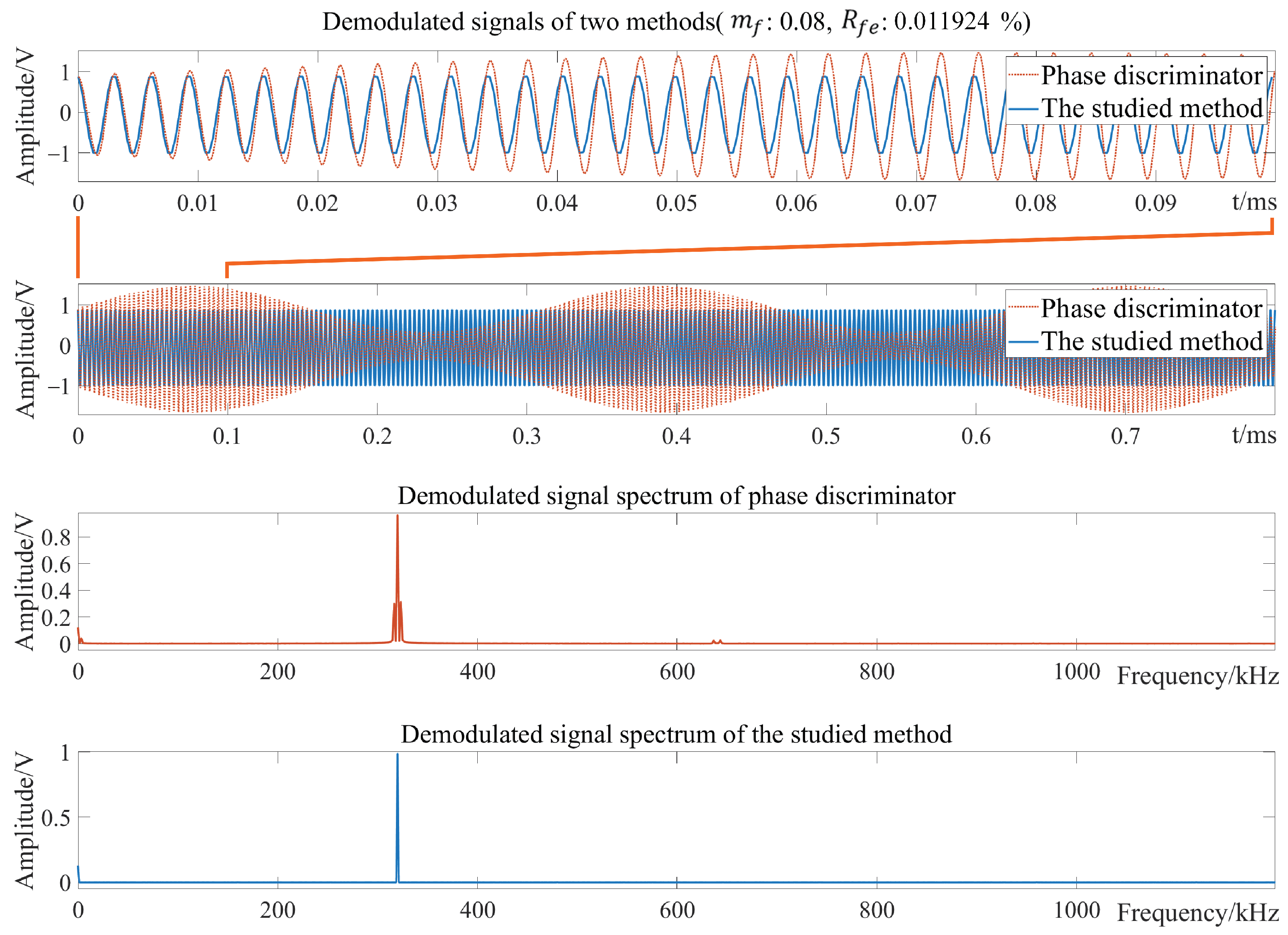
4.2. Influence of Carrier Center Frequency Error

As shown in

Table 4. Simulation conditions of FDD caused by carrier center frequency error.

Simulation Conditions	Value
$f_c$ (MHz)	13.20
$U_{cm}$ (V)	1.00
$m_f$	0.08
Maximum frequency offset ratio	0.1939%
$U_{\Omega m}$ (V)	1.00
SNR (dB)	60.00
$f_0$ (MHz)	3.2
$f_1$ (MHz)	12.8
$n_1$	4
$f_2$	19.2
$n_2$	6

, the conditions with a high frequency discrimination quality of the two methods are selected to test the influence of the carrier center frequency error on the frequency discrimination quality. Based on previous study, 40 sets of FM signal samples with different center frequency errors were selected for simulation.

Under different carrier center frequency errors, the frequency discrimination distortion and relative error of the two methods are tested as shown in

Table 5. FDD caused by center frequency error.

${\mathit{R}}_{\mathit{fe}}$ (%)	FDD of PD (%)	Relative Error (%)	FDD of MIFD (%)	Relative Error (%)	(${\mathit{R}}_{\mathit{fe}}$) (%)	FDD of PD (%)	Relative Error (%)	FDD of MIFD (%)	Relative Error (%)
0.000000	0.2570	0.00	0.0061	0.00	0.007492	1.4790	476.20	0.0062	1.64
0.000379	0.2960	15.40	0.0068	11.48	0.007727	1.5480	503.20	0.0062	1.64
0.000568	0.3540	37.80	0.0065	6.56	0.007962	1.6730	551.70	0.0067	9.84
0.000780	0.4380	70.60	0.0063	3.28	0.008197	1.8190	608.60	0.0064	4.92
0.000902	0.5030	95.90	0.0063	3.28	0.008432	2.0270	689.70	0.0059	−3.28
0.001023	0.5580	117.50	0.0069	13.11	0.008667	2.2880	791.20	0.0062	1.64
0.001144	0.6230	142.50	0.0061	0.00	0.008902	2.5780	904.40	0.0068	11.48
0.001265	0.7010	173.10	0.0064	4.92	0.009136	2.9500	1049.00	0.0063	3.28
0.001386	0.7740	201.50	0.0057	−6.56	0.009371	3.3750	1214.80	0.0063	3.28
0.001508	0.8530	232.30	0.0058	−4.92	0.009606	3.8510	1400.40	0.0070	14.75
0.001629	0.9190	258.10	0.0064	4.92	0.009841	4.3830	1607.50	0.0073	19.67
0.001750	1.0020	290.30	0.0062	1.64	0.010076	4.9740	1837.70	0.0059	−3.28
0.001871	1.0750	318.60	0.0071	16.39	0.010689	6.7600	2533.60	0.0063	3.28
0.001992	1.1520	348.90	0.0056	−8.20	0.011311	8.9050	3368.90	0.0060	−1.64
0.002114	1.2280	378.30	0.0064	4.92	0.011924	11.1530	4244.70	0.0061	0.00
0.002341	1.3610	430.10	0.0073	19.67	0.012545	13.4900	5155.00	0.0065	6.56
0.003902	1.8810	632.70	0.0063	3.28	0.013159	15.6030	5978.20	0.0061	0.00
0.005462	1.7010	562.60	0.0065	6.56	0.013780	17.3550	6660.70	0.0066	8.20
0.007023	1.4100	449.20	0.0061	0.00	0.014402	18.6480	7164.50	0.0069	13.11
0.007258	1.4330	458.30	0.0061	0.00	0.015015	19.3550	7439.90	0.0064	4.92

. Based on the simulation data, the frequency discrimination distortion–carrier center frequency error characteristics of the two frequency discrimination methods are plotted as shown in Figure 8. When the carrier center frequency error rate ($R_{fe}$) is 0%, the frequency discrimination distortion of the phase discriminator is 0.2570%, and the frequency discrimination distortion of the frequency discrimination method studied in this paper is 0.0061%. When the error occurs in the carrier center frequency, the frequency discrimination distortion of the phase discriminator increases in stages with the increase in the error. When the carrier center error rate is lower than 0.008432%, the frequency discrimination distortion of the phase discriminator shall not exceed 2.0270%. When the carrier center error rate exceeds 0.008432%, the frequency discrimination distortion of the phase discriminator increases exponentially, and the frequency discrimination quality drops sharply. However, under different carrier center frequency errors, the frequency discrimination distortion of the frequency discrimination method in this study is kept between 0.0056% and 0.0073%. In practical application, its frequency discrimination distortion mainly comes from noise interference, and the carrier center frequency has little influence on its frequency discrimination quality, which can be ignored.

It is observed through simulation that the demodulated signal of the phase discriminator is amplitude modulated when there is an error in the carrier center frequency. When the center frequency error of the carrier increases, the amplitude modulation phenomenon of the demodulated signal becomes more pronounced. When the carrier center frequency error rate is 0.011924%, the frequency discrimination result of the phase discriminator is observed as shown in Figure 9. The demodulated signal has obvious amplitude modulation characteristics, and the sum frequency and difference frequency components of amplitude modulation can also be detected in its spectrum. When the carrier center frequency error occurs, the demodulated signal of the two frequency discrimination methods will have a small DC offset, which is relatively easy to correct in practical applications. In addition, the demodulation signal obtained by the frequency discrimination method in this study has almost no other drawbacks.

In the frequency discrimination application of various basic frequency discriminators, the accuracy of the carrier center frequency is highly required. Tiny carrier center frequency errors caused by transmitter and noise interference during transmission will greatly affect the frequency discrimination quality of the frequency discriminator. The frequency discrimination method in this study effectively avoids the problem of carrier center frequency error.

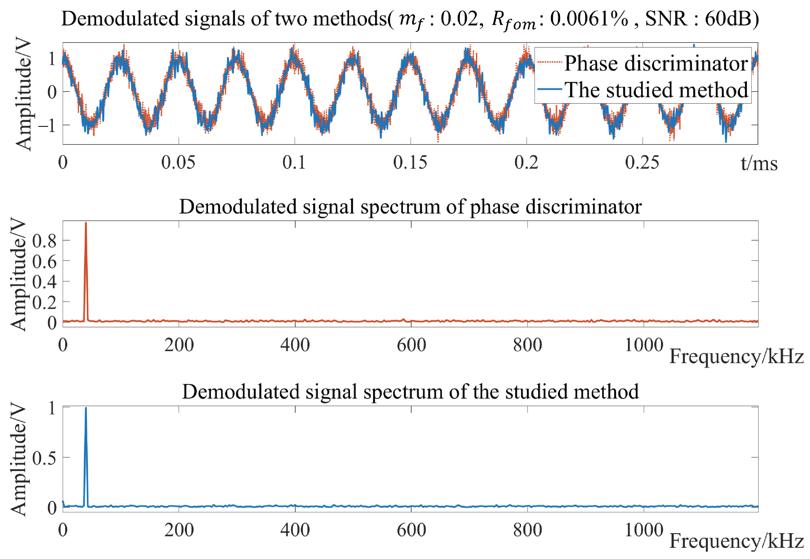
4.3. Anti-Noise Performance Analysis

To analyze the anti-noise performance of the two frequency discrimination methods, three groups of FM signals with smaller even harmonics of the phase discriminator are selected in the simulation to analyze the frequency discrimination distortion under noise interference with different signal-to-noise ratios. Their maximum frequency offset ratios are 0.0364%, 0.0968%, and 0.1575%, respectively. The SNR test range is set as 40 dB to 80 dB, and the frequency discrimination distortion affected by noise is:

$$\begin{array}{c}\hfill {\gamma }_{SNR}={\gamma }_T-{\gamma }_{\infty }\end{array}$$

(15)

where ${\gamma }_{SNR}$ is the frequency discrimination distortion caused by noise, ${\gamma }_T$ is the total frequency discrimination distortion, ${\gamma }_{\infty }$ is the frequency discrimination distortion when the SNR is infinite, that is, there is no noise effect. Through simulation, the noise characteristic curves of the two methods are drawn as shown in Figure 10.

The frequency discrimination distortion caused by noise decreases logarithmically with the increase in SNR. The greater the maximum frequency offset of FM signal, the stronger the anti-interference ability to noise. When the maximum frequency offset ratio in the simulation reaches 0.1575%, the frequency discrimination distortion of the two frequency discrimination methods caused by noise is lower than 1.454% when the SNR ratio is higher than 40 dB. Under each maximum frequency offset condition, the average reduction rate of the frequency discrimination distortion caused by the noise of the frequency discrimination method studied in this paper is 33.80% compared with the phase discriminator, which proves that the method studied in this paper has better anti-noise performance.

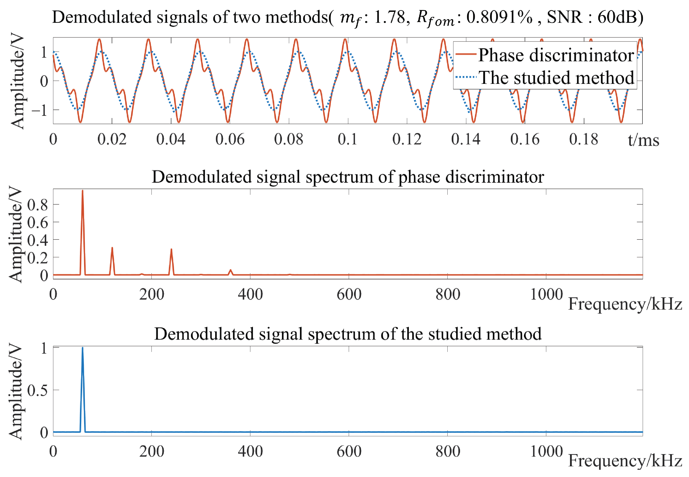
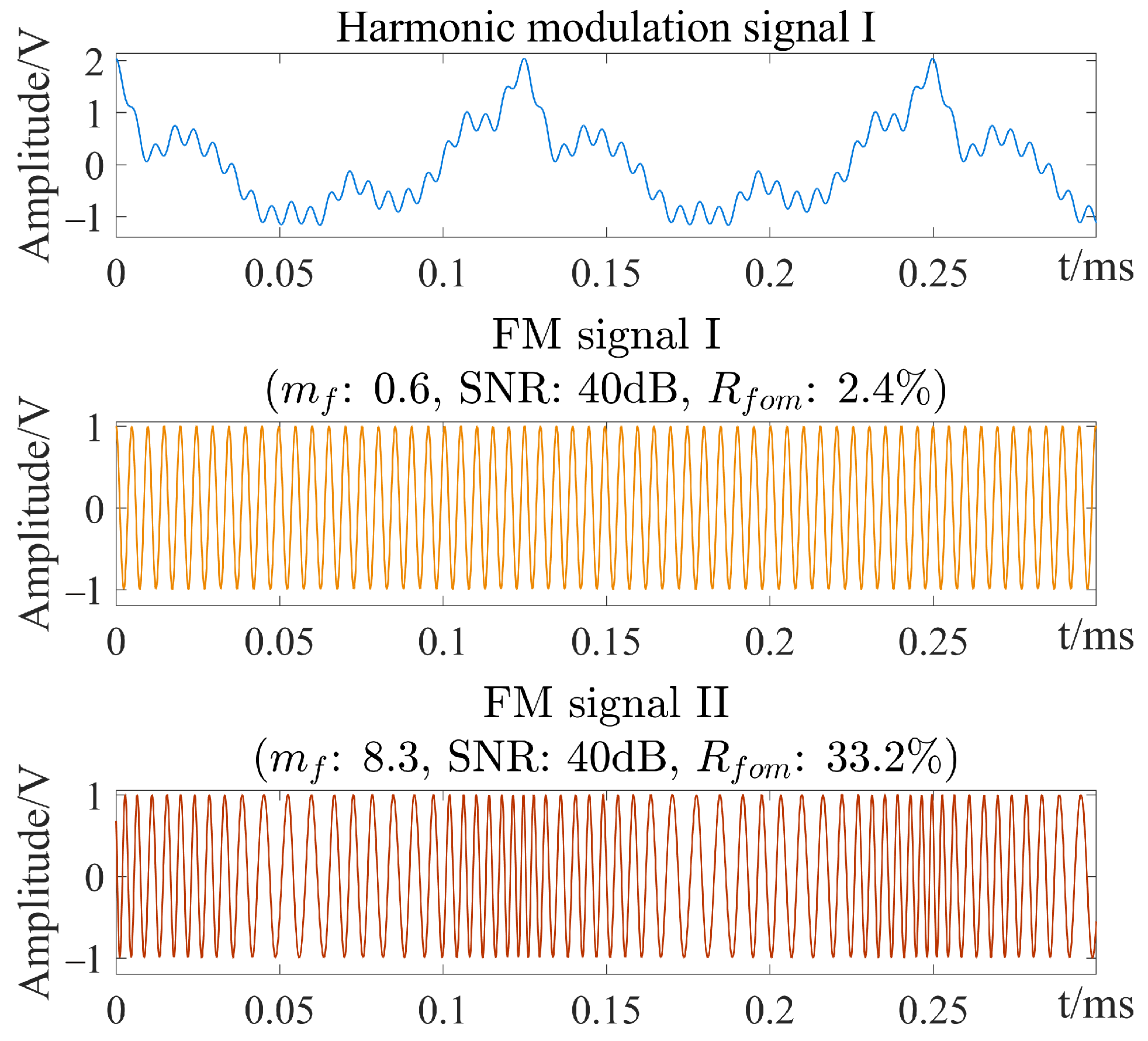
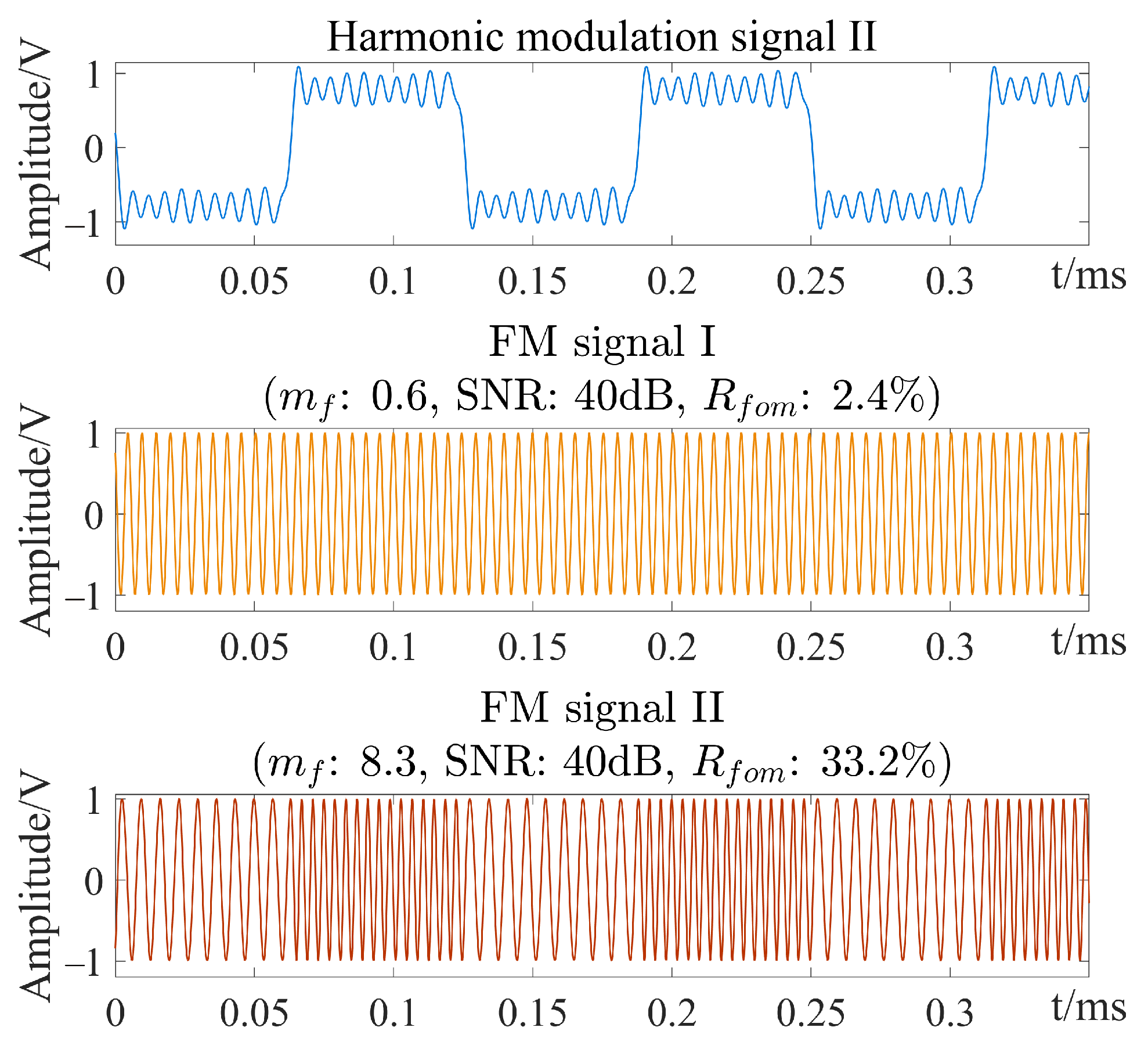
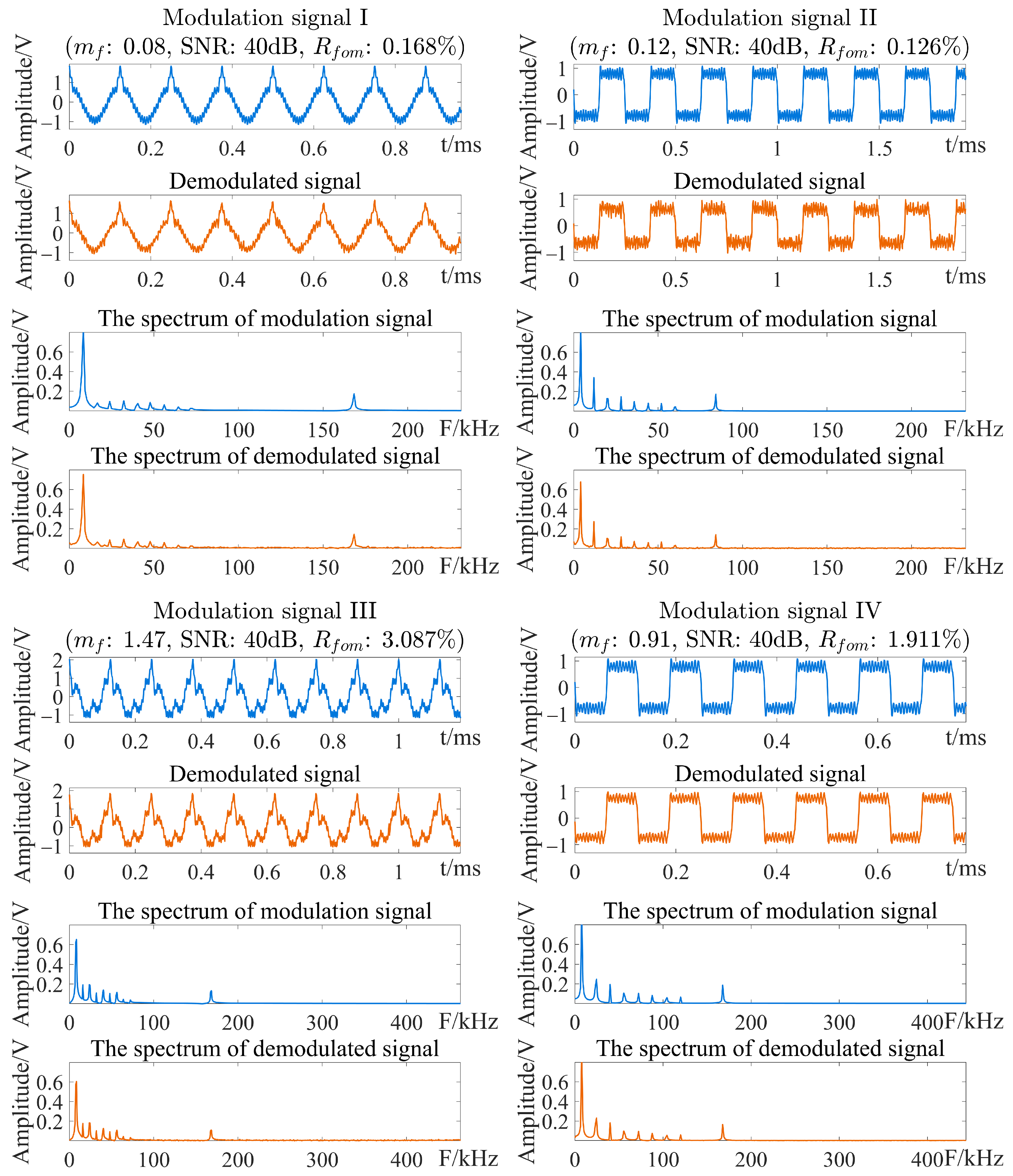
4.4. Frequency Discrimination Performance of FM Signal Modulated with Harmonic Signal

In practical applications, the modulation signal is usually not a single frequency signal but a harmonic, such as audio signal, image signal, etc. The FM signal generator in the simulation model can generate modulated signals that contain harmonics of different orders and amplitudes. The generated FM signals are shown in Figure 11 and Figure 12 (to demonstrate the frequency modulation effect, the carrier signal frequency $f_c$ is set low, and the maximum frequency offset ratio $R_{fom}$ is set high), and the highest harmonic order of the original modulation signal is 21.

Figure 13 shows the frequency discrimination results of the FM signals with four different FM indexes, maximum frequency offset ratios and lengths of window. From the spectrum, it can be seen that the harmonic component characteristics of the demodulated signal are consistent with the original modulated signal. Except for the extremely small frequency components brought in by noise, there is no obvious distortion. According to the method theory studied in the article, x is the carrier frequency parameter calculated by Equations (9)–(11) within one cycle of the signal with the maximum common divisor frequency of the selected differential frequency signals. It is not affected by the type and characteristics of the original modulation signal and the length of the calculation window.

5. Conclusions

The frequency discrimination method studied in this paper can accurately restore the original modulation signal through multiplicative-integration and linear transformation of the FM signal and preset two channel differential frequency signals. Due to not being affected by the type and characteristics of the modulation signal and the length of the calculation window, it can be used for frequency discrimination of multiple types of signals and has more obvious advantages in digital frequency discrimination [11] technology. Compared with the common frequency discrimination method, the method studied in this paper has better anti-noise performance and lower frequency discrimination distortion, and is less affected by the FM index, which reduces the limit on the bandwidth of FM signal and can meet more requirements for high bandwidth frequency discrimination applications. This method has low requirements for the accuracy of the carrier center frequency, that is, when the carrier center frequency has errors, it can still ensure the high quality of the demodulated signal, which solves the core problem that most common frequency discriminators are affected by the accuracy of the carrier center frequency, and can deal with the frequency errors in the transmission process of most FM signals, which is of great significance in the frequency discrimination technology.

References

1. Hu, Z.; Li, S.; Xiang, Y. Time Information Transmission Based on FM Broadcast Signal. IEEE Access 2021, 9, 16360–16364. [Google Scholar] [CrossRef]
2. Pound, R.V. Electronic Frequency Stabilization of Microwave Oscillators. Rev. Sci. Instrum. 2004, 17, 490. [Google Scholar] [CrossRef] [PubMed]
3. Wang, F.; Chen, X.; Men, A.; Zhang, L.; Wu, S. Carrier Frequency Offset Estimation for FM and Symbiotic FM Radio Data System Hybrid Signal. China Commun. 2020, 17, 129–139. [Google Scholar] [CrossRef]
4. Foster, D.E.; Seeley, S.W. Automatic Tuning, Simplified Circuits, and Design Practice. Proc. IEEE 1937, 25, 289–313. [Google Scholar] [CrossRef]
5. Sotner, R.; Polak, L.; Jerabek, J.; Petrzela, J.; Kledrowetz, V. Analog Multipliers-Based Double Output Voltage Phase Detector for Low-Frequency Demodulation of Frequency Modulated Signals. IEEE Access 2021, 9, 93062–93078. [Google Scholar] [CrossRef]
6. Salzenstein, P.; Wu, T.Y. Uncertainty analysis for a phase-detector based phase noise measurement system. Measurement 2016, 85, 118–123. [Google Scholar] [CrossRef]
7. Carr, J.; Frank, B. Static Phase Offset in a Multiplying Phase Detector. IEEE Microw. Wirel. Components Lett. 2009, 19, 518–520. [Google Scholar] [CrossRef]
8. Andersson, S. Frequency-discriminator-stabilized oscillators with common resonators. Microw. Opt. Technol. Lett. 1999, 21, 417–423. [Google Scholar] [CrossRef]
9. Hamdan, A.; Ros, L.; Hijazi, H.; Siclet, C.; Al-Ghouwayel, A. On multi-carrier systems robustness to Doppler in fast varying flat fading wireless channel. Digit. Signal Process. 2021, 117, 103189. [Google Scholar] [CrossRef]
10. Robson, S.; Tan, G.; Haddad, A. Low-Cost Monitoring of Synchrophasors Using Frequency Modulation. Energies 2019, 12, 611. [Google Scholar] [CrossRef]
11. Nakhostin, M. Digital discrimination of neutrons and γ-rays in liquid scintillation detectors by using low sampling frequency ADCs. Nuclear Instrum. Methods Phys. Res. Sect. A 2018, 916, 66–70. [Google Scholar] [CrossRef]
Figure 1. System model of the frequency discrimination method.
Electronics 13 01742 g001
Figure 2. Block diagram of simulation model.
Electronics 13 01742 g002
Figure 3. FM signal generated in MATLAB.
Electronics 13 01742 g003
Figure 4. Distribution diagram of frequency discrimination distortion.
Electronics 13 01742 g004
Figure 5. Frequency discrimination result ( m f = 0.02 ).
Electronics 13 01742 g005
Figure 6. Frequency discrimination result ( m f = 0.12 ).
Electronics 13 01742 g006
Figure 7. Frequency discrimination result ( m f = 1.78 ).
Electronics 13 01742 g007
Figure 8. Characteristic diagram of FDD–carrier center frequency error.
Electronics 13 01742 g008
Figure 9. Frequency discrimination result (center frequency error ratio 0.011924%).
Electronics 13 01742 g009
Figure 10. Noise characteristic curves of two methods.
Electronics 13 01742 g010
Figure 11. FM signal modulated with harmonic signal I with different m f .
Electronics 13 01742 g011
Figure 12. FM signal modulated with harmonic signal II with different m f .
Electronics 13 01742 g012
Figure 13. Frequency discrimination results of FM signals with harmonic signal with different conditions.
Electronics 13 01742 g013