Abstract
This article discusses the challenges in preventing workpiece damage due to impacts in electro-hydraulic loading systems, especially in unknown environments. We propose an innovative compliance control strategy, synergizing a series elastic actuator with impedance control to significantly mitigate impact forces between the mechanism and test workpieces. The controller consists of two loops: an internal loop and an outer loop. The internal loop integrates a position loop utilizing a radial basis function observer within a backstepping control framework, effectively countering the nonlinear dynamics of hydraulic actuators and ensuring precise trajectory tracking. The outer loop advances traditional impedance control by adaptively modifying the damping coefficient, resulting in a straightforward and easily implementable damping control law. For the unknown environment parameters, our system employs a parameter estimation law to estimate the unknown environmental stiffness and position parameters. The effectiveness of this strategy has been verified through comparative simulation with traditional impedance control, indicating that the proposed method can not only effectively reduce contact shock in unknown environments, improve response speed, and reduce overshoot, but also improve steady-state accuracy. We provided a feasible control scheme for similar systems to ensure precise and safe operation.
1. Introduction
The structural load testing system is mainly used to evaluate the performance of various materials, mechanical structures, or components under static or cyclic loading conditions. This system is used to simulate various loads that materials and structures may encounter in practice, providing a scientific method for evaluating structural design performance and identifying issues related to vibration and force excitation. As an important tool for engineers and researchers, it plays a crucial role in testing and validating performance benchmarks. By utilizing this system, potential fatigue failure mechanisms and design defects can be detected early, significantly improving the reliability and safety of engineering design. It can be applied in many fields, including automotive and aerospace industries [1], structural testing [2], civil engineering [3], and both civilian and military structural engineering, underscoring its versatility and importance in modern engineering practices.
Electro-hydraulic servo systems, known for their significant output force and high responsiveness, are widely used as power actuators in many loading test systems. However, the inherent nonlinearity, parameter uncertainties, and modeling uncertainties associated with these systems present complex challenges in the development of high-performance closed-loop controllers [4,5,6,7]. Moreover, within the specific framework of fatigue loading test systems, a critical area of research is the reduction in impact damage to test specimens during the testing process.
In traditional fatigue load testing systems, the end effector directly contacts the workpiece during task execution. Impact usually occurs during the transition from separation to contact between the experimental platform and the sample. Therefore, designing a reasonable end effector and compliant control strategy is crucial. To address the challenge of contact impact and achieve compliant control of contact force, many scholars have conducted research in this field. There are usually two methods to achieve compliance control: active compliant control and passive compliant control. Passive compliant control, in particular, can be effectively implemented by installing an elastic buffer device, such as a spring, at the end of the actuator. This approach is known as the series elastic actuator (SEA) [8,9], providing both anti-impact characteristics and high force fidelity for contact control. But achieving high-precision force tracking with the SEA remains a challenge. Mustalahti et al. [10] considered the nonlinear dynamics of the SEA, established a fifth-order state-space model for hydraulic systems, and designed a full-state feedback controller. Similarly, Zhong et al. [11] integrated the SEA and their dynamic models with a disturbance observer (DOB) to design a position controller for high-precision trajectory tracking.
However, a limitation in the existing research is that the parameters of the testing environment are known. In the context of load testing systems, environmental parameters such as stiffness often vary for different test specimens, making these methods less practical for scenarios where such parameters are unknown. To effectively adapt to diverse working environments and accurately evaluate environmental parameters, scholars have conducted significant research in this field. Misra et al. [12] employed adaptive techniques to estimate environmental parameters in the context of bilateral robotic arms. Their work involved the use of adaptive strategies to continually adjust to changing environmental conditions, enhancing the precision and effectiveness of robotic operations. Calanca et al. [13] developed an innovative environment-adaptive force controller. This controller operates by continuously modifying its control laws based on the real-time, online estimation of environmental dynamics. This method allows for more sensitive and accurate adaptation to changing environmental conditions, significantly improving the performance of the control system in different situations.
The above work and methods on contact force compliance control and environmental parameter estimation have laid the foundation for the research in this article. These advancements in adaptive control technology are essential for developing more sophisticated and responsive systems capable of operating efficiently in a wide range of environmental conditions. For hydraulic systems, the inherent challenges posed by high nonlinearity, significant parameter uncertainties, and modeling errors significantly complicate the design of high-performance force feedback control systems. Despite these challenges, various control strategies have been developed to achieve high-precision position control in such systems.
Among these strategies, adaptive control [14] has been widely researched for its ability to adjust to changing system dynamics. Robust control [15,16] is another approach that ensures system stability and performance despite uncertainties and disturbances. Disturbance observer-based control [17] effectively compensates for external disturbances, enhancing system accuracy. Adaptive sliding mode control [18] combines the benefits of sliding mode control and adaptive methods to handle system uncertainties effectively. Neural network control [19] employs artificial neural networks to model complex nonlinearities, offering a sophisticated approach to control hydraulic systems. Indirect adaptive backstepping control [20] integrates the robustness of backstepping control with the adaptability of indirect adaptive methods, making it particularly suitable for systems with uncertain dynamics.
Based on the above analysis, this article proposes a control strategy for an electro-hydraulic loading testing system. This scheme combines a series of elastic actuators with an impedance controller based on position control to reduce the impact on the loading process and improve the accuracy of loading force tracking. The design of the internal position loop controller is crucial, as it must provide high tracking accuracy and fast response speed, enabling the electro-hydraulic servo system to accurately and timely track and adjust its trajectory. In addition, in order to adapt to unknown external testing environments, a parameter estimation law is designed to obtain real-time external testing environment information. Finally, the effectiveness of the proposed loading test bench control system was verified through simulation.
The main contributions of this article are as follows:
(1) An impedance control strategy for series elastic actuators is proposed to address the issue of load force compliance control in electro-hydraulic servo loading systems. In order to improve the transient performance of the system in a stiffness environment model, a variable damping adaptive law is proposed.
(2) A parameter estimation law was proposed to obtain stiffness and position parameter information of the external testing environment, and a convergence proof of parameter estimation was provided to improve the ability of the loading system to adapt to unknown external testing environments and ensure the steady-state tracking accuracy of the loading force.
The remaining structure of the article is organized as follows: Problem formulation and dynamic models are presented in Section 2. Section 3 gives the output feedback model predictive controller design and the proof of stability. Section 4 introduces and discusses the results of numerical simulation experiments. Finally, Section 5 provides a summary and conclusion, encapsulating the findings and implications of the study.
2. Hydraulic Actuator System Description
2.1. Dynamics of Hydraulic Servo Loading System
Figure 1 shows the structure of the electro-hydraulic servo loading test system. The system uses a double acting hydraulic cylinder as the actuator; the system is equipped with linear variable differential transformer (LVDT) and force sensors, which are used to measure the displacement and output force of the hydraulic cylinder piston rod. In addition, the system is equipped with two pressure sensors that are responsible for obtaining the pressure values in the two chambers of the hydraulic cylinder. In order to achieve passive compliance control, the system combines the SEA at the end of the hydraulic cylinder actuator.
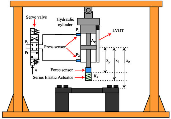
Figure 1.
The structure of the electro-hydraulic system.
In the design process of the impedance controller, researchers usually consider two environmental interaction models: the stiffness model [21] and the stiffness-damping model [22]. The stiffness model mainly focuses on characterizing the stiffness characteristics of objects. When dealing with energy dissipation caused by internal friction of materials, the stiffness model can not only show excellent accuracy but also achieve the goal of simplifying the model. The stiffness damping model takes into account the stiffness characteristics and damping effects of the object. Compared to the stiffness model, although it provides a more accurate description of the environment, it is more complex in terms of computation and implementation. Due to the fact that the test objects of the hydraulic loading test bench are mostly materials with low damping, such as metal materials, this article chooses a stiffness model to simulate the external testing environment.
The loading process is shown in Figure 2; the loading process can be divided into two different stages: “free-space state” and “contact state”. The difference between these stages is based on whether there is contact force between the hydraulic piston and the workpiece.
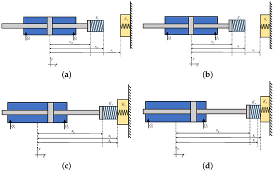
Figure 2.
Loading motion of the contact process. (a) Initial state; (b) Free-space motion; (c) Contact state; (d) Loading motion.
Figure 3 shows a schematic diagram of the impedance model. According to the principle of impedance control, the behavior of the end effector is characterized by a “spring–mass–damping” system. In this model, , and are the parameters of the required impedance model. These parameters are integral to the functioning of the system, dictating the dynamic response of the end effactor. Additionally, the workpiece environment parameters for external testing are denoted as , and the variable signifies the initial distance between the piston and the workpiece. represents the stiffness of the SEA.
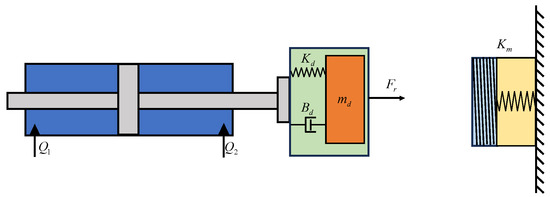
Figure 3.
Tracking errors of sine wave simulation.
Considering the SEA and the workpiece stiffness collectively, the total stiffness of the system can be expressed as
From (1), it can be seen that the total stiffness of the testing environment is inversely related to the stiffness of the SEA. This means that as decreases, also decreases. The reduction in the total stiffness of the system effectively reduces the instantaneous impact force when the actuator comes into contact with the test object.
Based on the above analysis, the dynamic model of the actuator of the hydraulic loading system can be described as follows
where represents the movement position of the hydraulic cylinder piston; represents the mass of the hydraulic cylinder piston; represents the pressure difference between two chambers; and and are the pressures inside the two chambers of the cylinder. represents the area of the piston; represents the effective viscous damping coefficient of the piston; and is defined as the unmodeled external disturbance, including external leakage, approximation error of the friction model.
The dynamic pressure model of the system can be expressed as follows
where is the total control volume of the hydraulic cylinder; is the effective oil bulk modulus; is the internal leakage coefficient; represents the modeling errors in the pressure dynamics; and is the load flow. and are the flow rates of the two chambers, they can be expressed as
where , is the density of the oil, is the discharge coefficient, and is the spool valve area gradient. Due to the fact that the bandwidth of the servo valve used in the system is much larger than that of the hydraulic system, the dynamic characteristics of the servo valve can be ignored and the input voltage is proportional to the displacement of the slide valve; that is , where is a positive gain. Then, the dynamic model of the servo valve can be written as follows
where represents the total flow gain of the servo valve, and u is the actual input voltage of the servo valve. The is defined as
2.2. Problem Formulation
The loading system actuator state variable is defined as: . Based on (1)–(5), the state-space expression of the system is as follows
where
Assumption A1.
The trajectory of the inner loop and bounded. In practical hydraulic systems under normal working conditions, the pressure of the two chambers is always bounded by , i.e.,
In addition, is smaller enough than to ensure that is far away from zero.
Assumption A2.
Parameters are unknown, but the upper and lower bounds are known
where , are known.
Assumption A3.
is globally Lipschitz with respect to .
Since the system is equipped with pressure sensors in two chambers, the pressure difference between the two chambers can be obtained in real time as . Therefore, if u is bounded, according to Assumption 1, it can be ensured that U is also bounded.
2.3. Projection Mapping and Parameter Adaptation
In the following sections, denote as an estimate of •, and denote as an estimation error of •. This article employs a discontinuous projection mapping to ensure that the estimated parameters remain within known upper and lower bounds. A discontinuous projection can be defined as
where , the adaptive law of design parameters is as follows
where is a positive constant and is an adaptive function, which will be designed later. By using discontinuous projections (10), for any designed adaptive function , the following two conditions will be guaranteed as
3. Controller Design
Due to the serious nonlinear characteristics of an electro-hydraulic servo system, impedance control strategies based on position are more suitable for such systems. This article proposes an output feedback control strategy for an electro-hydraulic servo system based on an RBF observer. This strategy utilizes an RBF neural network state observer to estimate the unmeasurable state of the system and estimates the uncertain parameters of the system by designing parameter adaptive laws, thereby achieving high-precision position tracking in the inner loop.
3.1. Design of State Observer Based on RBF Neural Network
The form of the designed RBF neural network state observer is as follows:
where denotes a design parameter that can be regarded as the bandwidth of the observer; , , and are observer design parameters. The parameters can be selected as , , and , respectively; is an estimate of . An unknown continuous nonlinear function can be represented by neural networks composed of ideal weights and a sufficient number of basis functions ; that is,
where is the neural network approximation error.
Assuming the ideal weights and basis functions are bounded as
Using neural networks to approximate is represented as follows:
where is the estimate of .
Theorem 1.
If the neural network observer is designed as (13), the design of the neural network adaptive law is (17), then it can be ensured that all state estimation errors and neural network weight estimation errors and are uniformly ultimately bounded (UUB). Moreover, all state estimation errors can converge to any small set by selected the bandwidth .
Proof.
See Appendix A. □
3.2. Inner Loop Position Controller Design
This section focuses on the design of a high-precision position controller for the inner loop of an electro-hydraulic servo system. In impedance control systems, the accuracy of the inner loop position controller directly affects the overall loading force tracking accuracy of the controller. The purpose of the inner loop controller is to ensure that the piston in the electro-hydraulic servo system can accurately and quickly track the required trajectory.
Step 1. The inner loop tracking error is defined as follows
Define the tracking error as
where is some positive feedback gain, is the virtual control law of state .
Step 2. Define the tracking error as
where is some positive feedback gain, is the virtual control law of state .
Combining (A1) and (20), it can be concluded that
Based on system model (7), the derivative of is as follows:
Therefore, the control law is designed as follows:
Substituting (23) into (22) yields
Then, the adaptive parameter estimation law is designed as follows
Theorem 2.
Given the design of the adaptive law (25), and by choosing the parameter sufficiently large to meet the condition (26), it can be ensured that all closed-loop system signals are bounded.
where are some positive numbers, as introduced in (A15).
Proof.
See Appendix B. □
Remark 1.
Through the designed high-precision inner loop position controller, it can be ensured that quickly tracks the desired ideal trajectory .
3.3. Adaptive Force Tracking in Unknown Environment
As seen in Figure 3, the force–displacement relation of the hydraulic actuator in free space and constrained space is
Defining the following variables, , and represent the reference trajectory and the command position trajectory, respectively. Based on the high-precision inner loop position controller designed earlier, it can achieve that in the position control mode. Defining as the designed contact force, the target dynamic equation of the impedance controller can obtain that
where , , and are the mass, damping, and stiffness coefficients of the expected impedance model. denotes the force tracking error, where is the reference force.
Performing Laplace transform on (28), combined with (27), yields
It can be seen from (29) that if zero steady-state error of loading force is achieved, the reference trajectory that can be designed is as follows:
Due to unknown environmental parameters, the estimated values of environmental parameters are used instead of the true values in (30). Denote and as the estimated values of and , respectively. Replacing with the estimated value in (30), one obtains
Then, the steady-state loading force tracking error becomes
From (32), it can be seen that the accuracy of obtaining environmental parameter information directly affects the steady-state error of loading force. Therefore, accurately estimating the environmental parameters of the system is of great significance for ensuring controller performance and improving loading force tracking accuracy. In addition, setting the expected stiffness to zero can also achieve the goal of zero steady-state error in loading force. However, as pointed out in [23], low expected stiffness will increase system overshoot and have a negative impact on the dynamic performance of the system. Therefore, this article does not adopt this method.
Defining as the estimated contact force, then the estimation error of is
Then the parameter estimation laws are designed as follows:
where , are some positive constants.
Proposition 1.
If satisfies the persistent exciting (PE) condition, the environment parameters and can converge to a small set of the actual value.
Proof.
Consider the following Lyapunov function as
Then, the derivation of can be computed as
Substituting (34) into (36), yields
Therefore, the estimated parameters and will converge to the set of the true values as , which completes the proof. □
The estimation of environmental parameters are achieved through the above methods, ensuring the steady-state error accuracy of the controller. In order to improve the response speed of the system and reduce the overshoot, an adaptive change law will be designed for the impedance model parameters of the system to improve the transient performance indicators.
Considering the impact of damping coefficient on control performance in the control system, this paper plans to adjust damping parameters by dynamically adjusting them. When the error is large, small damping is used to improve response speed, and when the error is small, damping is increased to limit system overshoot. After the system completes error correction and achieves a relatively ideal trajectory following, reduce the damping parameters of the model to address the upcoming error changes. The developed damping variation formula is as follows
where is the range of damping change, and is the initial damping coefficient. The definition of is as follows:
where is the set threshold.
Equations (38) and (39) indicate that the impedance model only adjusts the damping coefficient when the error rate of change is greater than the preset threshold . In cases of large errors, damping will be reduced to improve response speed. When the error is small, increase damping to reduce overshoot. When the rate of error change is below the threshold , it can be considered that the system has completed the transition process. At this point, the system will disable the damping adjustment function, thereby reducing the damping parameters of the impedance model. This error-based dynamic damping adjustment method not only improves the response speed of the system, but also reduces system overshoot, which is of great significance for improving the dynamic performance of the control system.
In summary, the complete variable impedance control framework can be obtained, as shown in Figure 4.
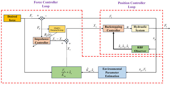
Figure 4.
Diagram of the proposed control algorithm.
4. Simulation Studies
To verify the effectiveness of the proposed control strategy, comparative simulation experiments were conducted in Simulink of Matlab to compare the performance of traditional impedance control strategy with the proposed variable impedance control strategy in this paper. The performance parameters of the hydraulic test bench in the simulation are shown in Table 1.

Table 1.
System parameters in numerical simulation.
Figure 5 shows the simulation program of the position-based force tracking impedance control strategy.
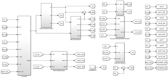
Figure 5.
Simulation diagram of the electro-hydraulic load test system in Matlab.
In the simulation case of this article, the lumped disturbance is set as follows:
The parameters setting for the inner loop position controller are as follows: , , and . The upper and lower bounds of unknown parameters are set as , . The initial value of is given as , the adaption rates of are selected as , , , , , and . The configuration for the RBF neural network observer is as follows: the bandwidth in (13) is selected as .
The traditional impedance control parameter selection is as follows: , , and , respectively. In the variable damping impedance control strategy, , , , and ; the other parameters are consistent with the traditional control strategy. To evaluate the performance of the two control strategies, the following indicators are used for evaluation: overshoot, rise time, adjustment time, and steady-state accuracy. This article will use the above parameters to conduct simulation analyses of four different working conditions.
4.1. Simulation of Constant Loading Force Tracking under Constant Environmental Parameters
This is the most basic loading condition, which involves tracking the constant loading force while keeping the environmental parameters constant. The expected load is 1000 N. The purpose is to verify the basic performance of the controller and the RBF observer for estimating unknown states. In this simulation case, the environmental position is set to m and the environmental stiffness is set to N/m. Figure 6 records the simulation results of loading force tracking, and Figure 7 describes the observation results of the RBF observer for unmeasurable states and . The control performance indicators of the two controllers are shown in Table 2.
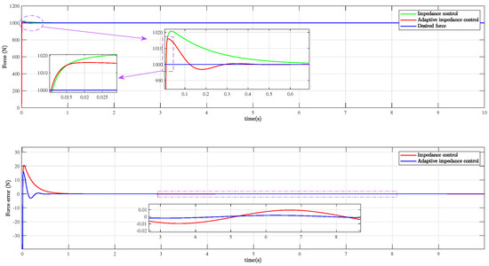
Figure 6.
Constant force tracking results in the constant environment.
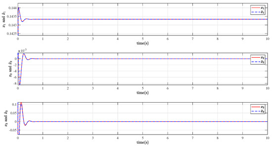
Figure 7.
Tracking performance of RBF state observer.
Table 2.
Comparison of performance parameters for constant force tracking in a constant environment.
From the comparison indicators in Figure 6 and Table 2, it can be seen that compared with traditional impedance control strategies, the proposed variable impedance control method has a significant improvement in the transient performance indicators of the control system, achieving both improved response speed and effective suppression of system overshoot. The maximum deviation is N, which is 22.8% lower than the N of traditional impedance control. At the same time, the steady-state index is also improved by 70% compared to traditional impedance control. It also entered a stable state in 0.5 s, which was significantly faster than the traditional impedance control of 1.2 s, achieving comprehensive improvement in both transient and steady-state performance indicators.
From Figure 7, it can be seen that the RBF state observer has an estimation effect on unmeasurable states, and it can be seen that the proposed RBF state observer can achieve estimation of states and .
4.2. Simulation of Stiffness Change under Constant Force
This section will compare the tracking performance of two control strategies when the stiffness of the simulated environment changes. The expected load is 200 N, and the stiffness will suddenly change from to when the simulation runs for 5 s. Figure 8 shows the tracking performance of two control strategies, while Figure 9 describes the estimation of stiffness. Table 3 compares the control performance indicators of two control strategies at the stiffness change point.
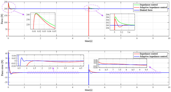
Figure 8.
Constant force tracking under changes in stiffness.
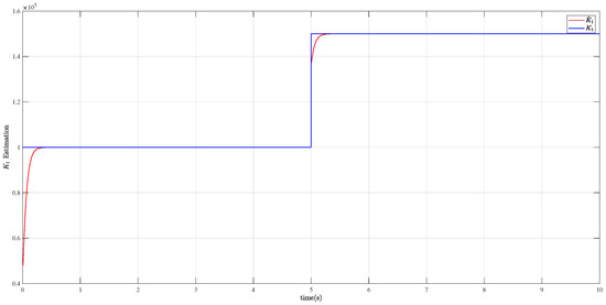
Figure 9.
Environmental stiffness estimation.
Table 3.
Comparison of performance parameters for constant force tracking in variable stiffness environments.
From Figure 8, it can be observed that when the external environmental stiffness suddenly changes at 5 s, the system bears a significant impact, but quickly returns to steady-state tracking. Specifically, the variable impedance control proposed in this article exhibits a smaller overshoot and faster convergence time when dealing with sudden changes in external environmental stiffness. Compared to traditional impedance control, the variable damping impedance control proposed in this article reduces overshoot by 24.5% during the adjustment process after stiffness mutation. The adjustment time has been reduced by 50%, indicating that the method proposed in this article has greatly improved both transient accuracy and steady-state accuracy. Figure 9 shows that the proposed environmental parameter estimation law can effectively track changes in external environmental stiffness.
4.3. Simulation of Step Loading Force Tracking under Constant Environmental Parameters
This section will compare the tracking performance of two control strategies under the step load spectrum when the simulation environment remains unchanged. The expected loading force curve is shown in Figure 10. Figure 11 shows the tracking performance of two control strategies, and Table 4 compares the control performance indicators of the two control strategies at the stiffness change point.
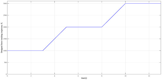
Figure 10.
Expected step loading force curve.
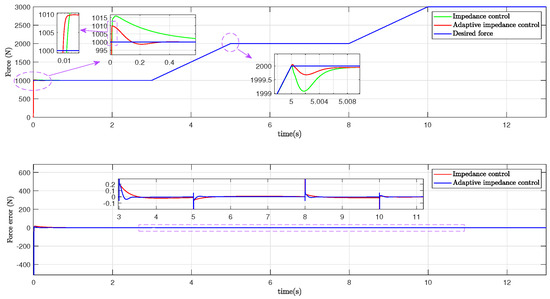
Figure 11.
Simulation results of step loading force tracking.
Table 4.
Comparison of performance parameters for constant environment step force tracking.
The stepped load spectrum represents the most prevalent test spectrum within loading systems. Observations from the simulation outcomes illustrated in Figure 11 reveal that, during the initial stages, the conventional fixed-parameter impedance controller manifests a significantly higher overshoot in response to abrupt changes in the loading force, and its rise time and settling time are inferior compared to the variable impedance controller introduced in this manuscript. At the 5 s mark, when the tracking trajectory experiences an abrupt transition, the novel variable impedance control approach delineated herein yields a diminished impact and expedited readjustment, showcasing enhanced adaptability to sudden alterations in the external environment in comparison to the traditional impedance control strategy.
4.4. Simulation of Alternating Loading Force Tracking under Constant Environmental Parameters
In fatigue testing, various alternating loads are often used for testing. This section will compare the tracking performance of two control strategies under alternating trajectories when environmental parameters remain unchanged. The expression for designing the loading force trajectory is as follows:
Figure 12 shows the tracking performance and error of two control strategies, while Table 5 compares the performance indicators of these two control strategies. In this case, the evaluation performance indicators used are the maximum tracking error, average error, and standard deviation during smooth operation.
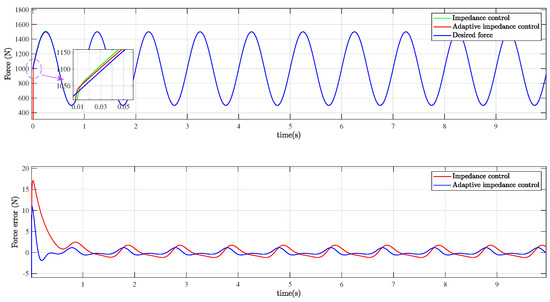
Figure 12.
Simulation results of sine loading force tracking.
Table 5.
Comparison of performance parameters for constant environment sine force tracking.
From Figure 12 and Table 5, it can be seen that the proposed variable damping control strategy exhibits better control performance under alternating loads due to its faster response speed. Compared to the impedance controller with fixed parameters, the maximum tracking error decreased by 33.7%, the average error decreased by 47.1%, and the standard deviation decreased by 66.7%. It can be seen that the overall control performance of the variable damping impedance control proposed in this article is superior to traditional fixed-parameter impedance control.
5. Conclusions
In this article, we introduce a new variable damping impedance tracking control framework. This framework aims to optimize the contact force control between the electro-hydraulic loading system and the environment. It is worth noting that the challenges faced here include the unknown stiffness and position of the environment, and the load spectrum to be tracked may be time-varying. By comparing the simulation case provided in the fourth section with traditional fixed-parameter impedance control, the superiority of the proposed variable damping impedance control system in transient and steady-state response was verified. The simulation results show that even in the presence of unknown environmental parameters, our controller can achieve high-precision loading force tracking for different load spectra. Even if the stiffness of the tested workpiece undergoes a sudden change, our proposed variable damping control strategy can still demonstrate excellent performance in reducing impact overshoot and adjustment time, providing reference experience for control system research similar to simulation platforms.
Moving forward, our efforts will concentrate on addressing the challenges of disturbance suppression during multi-channel simultaneous loading. Additionally, we plan to further validate and refine our algorithm through practical experiments using our constructed loading test bench.
Author Contributions
Conceptualization, H.S. and S.J.; methodology, S.J.; software, S.Z.; validation, H.S. and C.C.; formal analysis, H.R.; investigation, J.T.; writing—original draft preparation, S.J.; writing—review and editing, H.S.; visualization, S.J.; supervision, S.Z. All authors have read and agreed to the published version of the manuscript.
Funding
This research was funded by National Key Research and Development Programs of Funder grant number 2022YFB3404705.
Data Availability Statement
If the reader has a reasonable request, the first author of this article may be contacted for the data presented in this article.
Conflicts of Interest
The authors declare no conflicts of interest.
Appendix A
Proof of Theorem 1.
Based on system Equation (7) and observer (13), the dynamic equation of the observation error can be obtained as follows:
Define the variables as follows:
Combining (14)–(16), then the expression for dynamic error is as follows:
where
Because matrix is Hurwitz, there must exist a positive definite matrix , which satisfies the following formula:
Consider the Lyapunov function candidate
Combining (A3), the time derivative of V results in
Substituting (15) into (A4) yields
Since , and , , combining (17) yields
Combining (A8) and (A9), then the expression for dynamic error of (A7) is as follows:
where
Based on the above discussion, (A10) can be simplified as
Let . As long as holds, is negative. According to the Lyapunov extension theorem, both the system observer error and the NN weights and the estimate errors of the NN weights are uniformly ultimate bounded. □
Appendix B
Proof of Theorem 2.
Consider the following candidate Lyapunov function:
Based on (19)–(21), (24), and (25), we can infer its time derivative is that
According to Assumption 3, therefore
where are some known positive constants.
According to (19) and (21), this yields
Therefore, (A15) can be rewritten as
Combining (34) yields
where , is defined as
Based on the RBF observer designed in the previous section, it is known that is bounded. Then, can be upper bounded as
where D is a known constant.
By selecting appropriate , , and to make positive definite, it can be ensured that
where , in which denotes the minimum eigenvalues of a matrix.
Based on the above analysis and discussion, it can be ensured that all signals are bounded in closed-loop system, that is, the tracking error is bounded. Therefore, Theorem 2 holds. □
References
- Yao, J.; Dietz, M.; Xiao, R.; Yu, H.; Wang, T.; Yue, D. An overview of control schemes for hydraulic shaking tables. J. Vib. Control 2016, 22, 2807–2823. [Google Scholar] [CrossRef]
- Miao, C.; Wang, H.; Song, Y. The correlation between static strength and fatigue strength test and simulation. J. Phys. Conf. Ser. 2023, 2660, 012042. [Google Scholar] [CrossRef]
- Sepulveda, C.; Mosqueda, G.; Wang, K.-J.; Huang, P.-C.; Huang, C.-W.; Uang, C.-M.; Chou, C.-C. Hybrid simulation framework with mixed displacement and force control for fully compatible displacements. Earthq. Eng. Struct. Dyn. 2024, 53, 838–855. [Google Scholar] [CrossRef]
- Xu, Z.; Sun, C.; Hu, X.; Liu, Q.; Yao, J. Barrier Lyapunov function-based adaptive output feedback prescribed performance controller for hydraulic systems with uncertainties compensation. IEEE Trans. Ind. Electron. 2023, 70, 12500–12510. [Google Scholar] [CrossRef]
- Xu, Z.; Zhou, X.; Dong, Z.; Hu, X.; Sun, C.; Shen, H. Observer-based prescribed performance adaptive neural output feedback control for full-state-constrained nonlinear systems with input saturation. Chaos Solitons Fractals 2023, 173, 113593. [Google Scholar] [CrossRef]
- Chen, L.; Jiang, J.; Gao, W.; Wang, C.; Xu, W.; Ai, C.; Chen, J. Position control for a hydraulic loading system using the adaptive backsliding control method. Control Eng. Pract. 2023, 138, 105586. [Google Scholar] [CrossRef]
- Feng, H.; Ma, W.; Yin, C.; Cao, D. Trajectory control of electro-hydraulic position servo system using improved PSO-PID controller. Autom. Constr. 2021, 127, 103722. [Google Scholar] [CrossRef]
- Han, S.; Wang, H.; Tian, Y.; Yu, H. Enhanced extended state observer-based model-free force control for a series elastic actuator. Mech. Syst. Signal Process. 2023, 183, 109584. [Google Scholar] [CrossRef]
- Cao, X.; Aref, M.M.; Mattila, J. Design and control of a flexible joint as a hydraulic series elastic actuator for manipulation applications. In Proceedings of the 2019 IEEE International Conference on Cybernetics and Intelligent Systems (CIS) and IEEE Conference on Robotics, Automation and Mechatronics (RAM), Bangkok, Thailand, 18–20 November 2019; pp. 553–558. [Google Scholar]
- Mustalahti, P.; Mattila, J. Position-based impedance control design for a hydraulically actuated series elastic actuator. Energies 2022, 15, 2503. [Google Scholar] [CrossRef]
- Zhong, H.; Li, X.; Gao, L.; Dong, H. Position control of hydraulic series elastic actuator with parameter self-optimization. In Proceedings of the 2019 IEEE 4th International Conference on Advanced Robotics and Mechatronics (ICARM), Toyonaka, Japan, 3–5 July 2019; pp. 42–46. [Google Scholar]
- Misra, S.; Okamura, A.M. Environment parameter estimation during bilateral telemanipulation. In Proceedings of the 2006 14th Symposium on Haptic Interfaces for Virtual Environment and Teleoperator Systems, Alexandria, VA, USA, 25–26 March 2006; pp. 301–307. [Google Scholar]
- Calanca, A.; Fiorini, P. Understanding environment-adaptive force control of series elastic actuators. IEEE/ASME Trans. Mechatronics 2018, 23, 413–423. [Google Scholar] [CrossRef]
- Mesbah, M.A.; Sayed, K.; Ahmed, A.; Aref, M.; Elbarbary, Z.M.S.; Almuflih, A.S.; Mossa, M.A. Adaptive Control Approach for Accurate Current Sharing and Voltage Regulation in DC Microgrid Applications. Energies 2024, 17, 284. [Google Scholar] [CrossRef]
- Ge, Y.; Zhou, J.; Deng, W.; Yao, J.; Xie, L. Neural network robust control of a 3-DOF hydraulic manipulator with asymptotic tracking. Asian J. Control 2023, 25, 2060–2073. [Google Scholar] [CrossRef]
- Nguyen, M.H.; Ahn, K.K. Output Feedback Robust Tracking Control for a Variable-Speed Pump-Controlled Hydraulic System Subject to Mismatched Uncertainties. Mathematics 2023, 11, 1783. [Google Scholar] [CrossRef]
- Lee, W.; Chung, W.K. Disturbance-observer-based compliance control of electro-hydraulic actuators with backdrivability. IEEE Robot. Autom. Lett. 2019, 4, 1722–1729. [Google Scholar] [CrossRef]
- Feng, H.; Song, Q.; Ma, S.; Ma, W.; Yin, C.; Cao, D.; Yu, H. A new adaptive sliding mode controller based on the RBF neural network for an electro-hydraulic servo system. ISA Trans. 2022, 129, 472–484. [Google Scholar] [CrossRef] [PubMed]
- Wan, Z.; Yue, L.; Fu, Y. Neural network based adaptive backstepping control for electro-hydraulic servo system position tracking. Int. J. Aerosp. Eng. 2022, 2022, 3069092. [Google Scholar] [CrossRef]
- Kaddissi, C.; Kenne, J.P.; Saad, M. Indirect adaptive control of an electrohydraulic servo system based on nonlinear backstepping. IEEE/ASME Trans. Mechatronics 2010, 16, 1171–1177. [Google Scholar] [CrossRef]
- Li, E. The robotic impedance controller multi-objective optimization design based on Pareto optimality. In Proceedings of the Intelligent Computing Methodologies: 12th International Conference, ICIC 2016, Lanzhou, China, 2–5 August 2016; Proceedings, Part III 12. Springer: Cham, Switzerland, 2016; pp. 413–423. [Google Scholar]
- Roveda, L.; Vicentini, F.; Tosatti, L.M. Deformation-tracking impedance control in interaction with uncertain environments. In Proceedings of the 2013 IEEE/RSJ International Conference on Intelligent Robots and Systems, Tokyo, Japan, 3–7 November 2013; pp. 1992–1997. [Google Scholar]
- Ji, W.; Tang, C.; Xu, B.; He, G. Contact force modeling and variable damping impedance control of apple harvesting robot. Comput. Electron. Agric. 2022, 198, 107026. [Google Scholar] [CrossRef]
Disclaimer/Publisher’s Note: The statements, opinions and data contained in all publications are solely those of the individual author(s) and contributor(s) and not of MDPI and/or the editor(s). MDPI and/or the editor(s) disclaim responsibility for any injury to people or property resulting from any ideas, methods, instructions or products referred to in the content. |
© 2024 by the authors. Licensee MDPI, Basel, Switzerland. This article is an open access article distributed under the terms and conditions of the Creative Commons Attribution (CC BY) license (https://creativecommons.org/licenses/by/4.0/).