Abstract
In the past decade, artificial neural networks (ANNs) have been widely employed to address many problems. Despite their powerful problem-solving capabilities, ANNs are susceptible to a significant risk of stagnation in local minima due to using backpropagation algorithms based on gradient descent (GD) for optimal solution searching. In this paper, we introduce an enhanced version of the reptile search algorithm (IRSA), which operates in conjunction with an ANN to mitigate these limitations. By substituting GD with IRSA within an ANN, the network gains the ability to escape local minima, leading to improved prediction outcomes. To demonstrate the efficacy of IRSA in enhancing ANN’s performance, a numerical model of the Nam O Bridge is utilized. This model is updated to closely reflect actual structural conditions. Consequently, damage scenarios for single-element and multielement damage within the bridge structure are developed. The results confirm that ANNIRSA offers greater accuracy than traditional ANNs and ANNRSAs in predicting structural damage.
1. Introduction
In recent years, structural health monitoring (SHM) has gained significant attention from scientists, particularly in the realm of nondestructive health monitoring methods. Regular health monitoring and tracking enable managers to easily plan maintenance and repairs for structures. One nondestructive health monitoring method that has garnered special attention from scientists in the diagnosis or prognosis of structural damage is the artificial neural network (ANN) [1,2,3].
The ANN is an advanced computational method developed based on the principles of human biological neural systems, particularly in information processing. With significant advancements in recent times, ANNs have become popular in solving complex problems across various fields. However, ANNs still have certain limitations. ANNs rely on the backpropagation (BP) algorithm based on gradient descent (GD), particularly in its simplest form (vanilla GD), which tends to become stuck at the local minima of the loss function, especially when dealing with complex and nonconvex error surfaces [4]. This can prevent GD from finding the global optimal solution in the parameter space of the ANN. Another reason why GD tends to become stuck at local minima is that traditional GD uses a fixed learning rate, which may not be ideal in every situation and can lead to very slow convergence. Therefore, providing a mechanism for the dynamic adjustment of the learning rate can help the model learn more effectively and converge more quickly.
To address this issue, the approach of using optimization algorithms with global search capabilities has been adopted by many researchers to create a better starting point for the algorithm. One approach is to prevent complex coadaptations of feature detectors, which can lead to local minimum problems [5]. Another solution involves the use of deep belief network (DBN) models to improve the ability of ANNs to forecast exchange rates by addressing issues such as determining initial weight values and long convergence times [6]. Moreover, the use of algorithms such as the hill-jump algorithm and mean-field theory in Hopfield neural networks has been explored to mitigate local minimum problems in combinatorial optimization and logical programming [7,8]. One of the most common approaches to solving the limitations of gradient-based optimization methods is using metaheuristic algorithms, including evolutionary algorithms and swarm intelligence, which have been widely investigated to obtain generalized feedforward neural networks (FNNs) for specific problems due to the limitations of gradient-based optimization methods [9]. Additionally, the application of particle swarm optimization (PSO), genetic algorithms (GAs) or hybrid algorithms has been shown to effectively address local minimum problems in the training processes of neural networks [10,11,12]. Furthermore, the susceptibility of algorithms like grey wolf optimization (GWO) to local optima and slow convergence has been noted, resulting in degraded performance [13].
The need for new algorithms to address these challenges arises from the inherent limitations of the existing metaheuristic approaches when combined with an ANN. For instance, the entrapment in local minima and slow convergence can hinder the overall performance and effectiveness of the optimization process [4]. Moreover, the combinatorial explosion of the search space in certain problems can lead to metaheuristic algorithms falling into local optima, further emphasizing the need for alternative approaches [14]. Additionally, the limitations of existing metaheuristic optimization algorithms, such as GWO, in overcoming local minima underscore the necessity for novel methods to enhance the optimization process and avoid performance degradation [13].
To overcome the shortcomings of traditional ANNs and the need for a new algorithm to replace the old, conventional ones when working in parallel with ANNs, in this paper, we propose a new ANN model operating in conjunction with the reptile search algorithm (RSA) [15]. Moreover, in this study, we also developed an improved version of the RSA. This version not only enhances the search efficiency of the algorithm by optimizing the selection and update paths of the ‘reptiles’ but also introduces a dynamic adjustment mechanism to enhance adaptability to various types of data and problems. This improvement allows the model to integrate seamlessly with the structure of ANN, enabling both algorithms to evolve together, leveraging the strengths of each approach to achieve higher performance in solving complex problems.
To demonstrate the effectiveness of ANNIRSA, a series of experiments assessing the level and capability of damage detection in structures using the algorithm were conducted in practical applications. To substantiate the efficacy of the proposed methodology, comparative analyses between ANNIRSA, ANNRSA, and conventional ANN were conducted across an array of damage scenarios simulated by the numerical model. The outcomes revealed that ANNIRSA surpassed both ANN and ANNRSA in terms of search ability and accuracy of prediction in all evaluated cases. The computational tasks in this study were carried out using a 12th Gen Intel(R) Core™ i7-12700F processor (https://ark.intel.com/content/www/us/en/ark/products/134592/intel-core-i7-12700f-processor-25m-cache-up-to-4-90-ghz.html, accessed on 22 March 2024) (20 CPUs), Intel, clocked at approximately 2.1 GHz. The primary contributions of this research are outlined as follows:
- We developed an enhanced IRSA algorithm integrated with an ANN.
- We successfully implemented the ANNIRSA algorithm for diagnosing structural damage.
- We extracted a new dataset of damages from the Nam O bridge model, encompassing a range of designated damage elements.
- We evidenced the precision and efficacy of the advanced methodology via a comprehensive suite of numerical simulations and empirical evaluations, encompassing a spectrum of scenarios ranging from isolated- to multiple-damage instances.
- We executed a systematic comparative evaluation of the advanced ANNIRSA method relative to established algorithms, notably, the traditional ANN and ANNRSA.
The subsequent sections of this paper are methodically structured for academic rigor. Section 2 elucidates the underpinnings of ANN and RSA, delves into the intricacies of the proposed IRSA, and articulates its concurrent operationalization with the ANN. In Section 3, we describe the construction of numerical examples and the dataset, meticulously curated from the Nam O bridge model. Section 4 is dedicated to presenting a comprehensive analysis of the empirical results, encompassing both singular- and multiple-damage scenarios, highlighting the efficacy of the proposed methodology. This paper culminates with Section 5, which synthesizes the key findings of this investigation and delineates prospective avenues for further scholarly exploration.
2. Materials and Methods
In this section, we expound on the ANN and RSA concepts. Here, the strengths and weaknesses of these methodologies are articulated, along with strategies for their mitigation. In the case of the traditional RSA, a series of modifications have been employed to enhance its performance, including:
- Adaptive alpha and beta values;
- A reduction function based on the global best solution;
- The incorporation of chaotic random sequences;
- Adaptive hunting probability;
- The implementation of a killer hunt strategy.
These refinements have transformed the RSA into a more formidable algorithm, which we refer to as the improved RSA (IRSA). The IRSA algorithm was integrated with ANN to augment the performance efficiency of ANNs.
2.1. Artificial Neural Network
In recent decades, ANNs have emerged as a revolutionary force in the fields of artificial intelligence and machine learning, marking significant advancements across various domains and garnering special attention from the scientific community. Within the realm of SHM, ANNs have facilitated the high-precision detection of damage, even with minimal datasets, where the output involves only a single neuron. However, when dealing with outputs involving more than one neuron, ANNs face challenges in accurately diagnosing damage for such types of output data. This difficulty may stem from the ANN’s reliance on the BP algorithm, which utilizes GD-based learning techniques to seek optimal solutions. This approach poses a significant risk of the network becoming trapped in local minima. The ANN architecture is depicted in Figure 1.
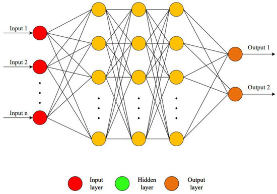
Figure 1.
ANN architecture.
The efficacy of an ANN predominantly hinges on whether the network resides within the most favorable local minima. Hoa et al. [12] posited that the strategic selection of an initial starting point merely serves to assist the network in navigating around local minima within a subset of rudimentary problems. Consequently, this methodology has been adopted by numerous researchers to address the local minima challenges encountered by ANNs [16,17]. While this approach proves to be quite effective in simpler problems, characterized by a limited number of optimal local solutions, it tends to falter in more complex scenarios that encompass a wide distribution of local minima. Therefore, it is imperative to devise strategies enabling the network to escape local optima regions, even when the initial points are unfavorable or random. In this paper, we advocate for the utilization of the random search capabilities of the RSA to tackle the issue of ANNs becoming trapped in suboptimal local minima.
2.2. Reptile Search Algorithm (RSA)
The RSA is a metaheuristic optimization technique that draws its inspiration from the hunting patterns of crocodiles in the natural world. This algorithm was recently introduced by Laith et al. [15]. It involves two main phases—encircling and hunting. The encircling phase is about exploration to search the global space, utilizing two strategies—high walk and belly crawl. The predatory phase is primarily oriented toward exploitation, aiming to zero in on the most favorable solution. This phase harnesses both coordinated and collaborative hunting tactics. Predominantly, these hunting strategies involve ambush techniques; many of such activities are nocturnal, often occurring in shallow aquatic environments. The mathematical representation of the solutions in RSA can be denoted as
where denotes the solution set, represents the ith solution at the jth position, is the number of solutions, and is the number of positions (dimensions).
In the initial stage of the predatory sequence, known as the encircling phase, crocodiles exhibit a dual-modality locomotion strategy, comprising high walk and belly crawl maneuvers. This dual approach facilitates a comprehensive exploration of the expansive search terrain, while maintaining a strategic distance from the prey, thereby avoiding premature disturbance. The search phase depends on two conditions: high walk when and belly crawl when and . The position can be described with an equation as follows:
where represents the jth position in the best solution obtained so far. The term rand denotes a random number within the range . The variable refers to the current iteration, and signifies the maximum number of iterations. The term is a random number within the range . is the number of candidate solutions. The notation signifies the random position of the ith solution. Lastly, denotes the jth position of the individual hunter in the ith solution, and the formulation is presented as
where is a sensitivity parameter; is a reduction function used to narrow the search area. The equation determining can be described as
Evolutionary sense denotes the likelihood of adopting values that diminish randomly, falling in the range of [−2, 2], across the iteration span, as determined by the following formula:
where is a small value, is a random number in the range , and 2 is used as a correlational value to generate values from 2 down to 0. is an integer random number in the range . quantifies the proportional discrepancy between the best solution’s jth position and the current solution’s jth position, ascertained as
where is the upper bound of the jth position; is the lower bound of the jth position. is established as a constant sensitivity coefficient, designated with a value of 0.1.
The mean position of the ith solution is which is calculated using Equation (7).
The second phase of the predation process is the hunting stage. During this phase, two main strategies are utilized: synchronized coordination and collaborative effort. These techniques enhance the localized search for solutions by intensifying efforts near the prey, diverging from the broader exploratory encircling phase. As a result, RSA’s exploitation phase is adept at uncovering near-optimal solutions through persistent trials and leverages communication between strategies to intensify the search near the best solution. These mechanisms, characterized by coordination and cooperation, optimize the search space to pinpoint the optimal solution, as depicted in Equation (8).
The position signifies the jth coordinate of the optimal solution thus far. The hunting operator corresponds to the jth position in the ith solution, as computed using Equation (3). The percentage difference between the optimal solution’s ith position and the current solution’s jth position is determined using Equation (6). The parameter , used to diminish the search zone, is derived from Equation (4).
The decision to employ either hunting strategy is predicated on specific conditions: coordination is utilized when falls within to , and cooperation is engaged otherwise, particularly when exceeds . Stochastic elements are integrated to explore and exploit the most auspicious local zones. This study adopted rudimentary principles that encapsulate the predatory patterns of crocodiles and introduced equations for updating positions during the exploitation phase.
The strategies for hunting are devised to avoid entrapment in local optima, thereby assisting the exploratory phase in locating the best solution while ensuring a variety of potential solutions remain available. The parameters and are finely tuned to produce stochastic values at every iteration, promoting continuous exploration across the algorithm’s runtime. This approach is especially beneficial in navigating past local optima stagnation, notably during the advanced stages of the algorithm’s execution.
2.3. Improved RSA
A series of enhancements were incorporated into the traditional RSA algorithm to refine its functionality. We began with the transition from fixed parameters to adaptive control parameters for more dynamic regulation. Unlike the static control parameters and in the original RSA, the improved version introduces self-adjusting parameters that evolve with the progression of iterations:
This adaptation ensures extensive initial exploration via high and values that gradually decrease to allow for more precise exploitation later.
The method also introduces an adaptive reduce function: the conventional reduce function is reformed to concentrate on the globally best solution instead of a random one:
This adjustment directs the search toward the optimal solution found thus far. Furthermore, the algorithm substitutes random sequences with chaotic maps such as logistic, tent, or sine maps to bolster exploration and sidestep suboptimal solutions. In this study, the logistic map, a classic example of a chaotic system, was mathematically represented as
Here, represents the value at the kth iteration, and is the system parameter, which was set to 4 in this context to exhibit chaos.
Additionally, an adaptive hunting probability parameter, , is integrated, dictating the transition likelihood from exploration to exploitation during iterations:
This incrementally amplifies exploitation probabilities as the algorithm advances.
The equation for updating the solution’s position was also simplified, no longer divided into four phases as before, which rendered the algorithm overly complex. To streamline the equation, the improved algorithm only utilizes Equations (2) and (8). The specific form of the updated equation is as follows:
Periodic ‘killer hunts’ are also employed, wherein the least-effective solution is culled and supplanted with a fresh random candidate, fostering diversity within the solution pool. The frequency of such interventions is adjustable.
Collectively, these refinements significantly bolster the capabilities of the original RSA. Adaptive control mechanisms autonomously modulate the balance between exploration and exploitation, while chaotic dynamics and ‘killer hunts’ ensure a rich diversity of solutions. These features, combined with the focus on the global best and the adaptable hunting probability, are anticipated to accelerate convergence and enhance overall performance. Figure 2 provides a comprehensive and detailed visualization of the IRSA methodology.
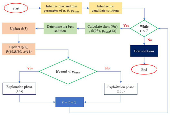
Figure 2.
Flowchart of IRSA.
2.4. Proposed Hybrid ANN and IRSA Method
In this section, the ANNIRSA methodology is delineated. Initially, the ANN is initialized, with the input layer receiving the raw input data. Here, the raw data are formatted as a vector , where each denotes the discrete features of the input. This vector acts as the cornerstone for the commencement of the forward propagation process.
Subsequently, the data proceed to the hidden layers. Within these layers, the network executes a twofold operation, commencing with a linear transformation. In this process, the input from the preceding layer, or the initial input in the case of the first hidden layer, is subjected to a linear transformation employing weights and biases. This operation is mathematically articulated as follows:
where denotes the output of the linear transformation at layer , while and represent the weights and biases associated with that layer. The term refers to the activation from the preceding layer, with equating the input vector .
After this step, an activation function is applied. The result of the linear transformation is subjected to this function, thereby injecting nonlinearity into the model. This is a critical feature, as it empowers the network to capture and represent complex patterns within the data.
where is the activation function for layer .
This procedure is iteratively conducted until the output layer is reached. At this juncture, a final transformation occurs, where the output of the last hidden layer is processed by the output layer to yield the ultimate output of the network.
At this point, the error between the output results and the predicted values is computed. For each data point , the squared difference is calculated between the predicted output (an element of ) and the actual target . The error metric, computed using the mean squared error (MSE) for data points, is determined by the following equation:
Should the network become trapped in a local optimum, it implies that the discrepancy between the predicted and actual outputs for a subsequent step does not exhibit a reduction compared to the preceding step.
In this scenario, the IRSA is employed to assist the network in navigating away from local optima. More precisely, the IRSA is used to optimize the weights and biases within the ANN framework. The aggregate count of variables requiring optimization is determined through the application of Equation (19):
where represents the total number of weights and biases that require optimization in the ANN. is the number of input nodes depending on the input data; are the number of nodes in the ith hidden layer; and is the number of output nodes based on the network’s output data. In this context, according to Equation (1), is essentially the dimensionality that the optimization algorithm aims to address.
Once the variables are incorporated into the IRSA, the steps are carried out as outlined in the flowchart in Figure 1. The objective function of the algorithm is Equation (15). The outcome of this process is the optimized weights and biases. The details of this procedure are presented in Figure 3.
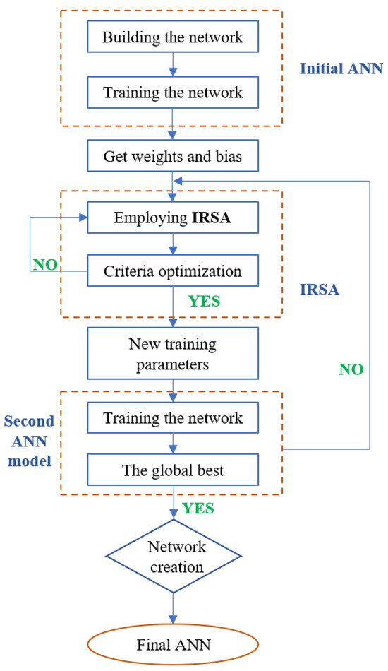
Figure 3.
Flowchart of ANNIRSA.
Subsequently, to generate input data for the network, a bridge structure was modeled, and simulations were conducted to replicate various potential damage scenarios across a group of elements. These data were then employed as the input for ANN, ANNRSA, and ANNIRSA, facilitating a comprehensive assessment of the network’s performance under different structural health conditions. This simulation-based approach provided a robust dataset, instrumental for the effective training and evaluation of the neural network models in structural damage detection and assessment tasks.
3. Numerical Examples
3.1. Description of the Bridge
Located centrally in Vietnam, the Nam O Bridge serves as an essential connector for rail transport between the north and south. Operational since 1950, it has consistently managed the high-frequency transportation of heavy train loads. Despite experiencing deterioration due to rust and other defects impacting some of its truss elements, leading to a decrease in stiffness or Young’s modulus, the bridge remains operational under its intended load capacities. It consists of four nearly identical spans, each measuring about 75 m, and features U-shaped abutments and solid shaft piers typical of railway bridges. The spans of the bridge are supported by roller and pin bearings. Its main structural components comprise both upper and lower chords, along with vertical and diagonal elements. Additionally, the structure incorporates upper and lower wind bracings, struts, and stringers. For a comprehensive breakdown of the truss members’ dimensions, one can refer to the details provided in Ref. [18]. The bridge’s design and layout are illustrated in Figure 4.
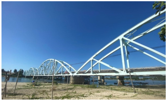
Figure 4.
Nam O Bridge.
3.2. Dataset
In this section, we introduce the numerical model of the Nam O Bridge (Figure 5), developed using the Stabil toolbox integrated within MATLAB software version 2022a [19]. The model incorporated 175 beam elements, each embodying six degrees of freedom at their nodes, encompassing both translational and rotational displacements. These elements collectively represent the truss components of the structure, cumulatively amounting to 300 degrees of freedom. The boundary conditions of the bridge were defined with fixed bearings at nodes 10000, 20000, 30000, and 40000, and sliding bearings at nodes 10160 and 30160.
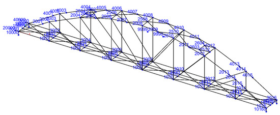
Figure 5.
FEM of Nam O Bridge.
To simulate damage scenarios, various element damage combinations were incorporated into the model using the Young’s modulus of selected elements. The damaged elements considered included 1000, 1003, 1006, 1009, 1012, 1015, 1018, and 1021. Different damage cases were created by damaging one or two elements in each scenario, with damage levels varying from a 1% to 50% reduction in the Young’s modulus. The total number of damage scenarios can be calculated using the following formula:
Here, represents the total number of samples, i.e., the number of damage scenarios; is the number of elements damaged simultaneously (e.g., for single-element damage cases); is the maximum percentage of the damage scenarios; and is the number of elements considered damaged in each case.
Thus, for single-element damage cases, the different combinations of 8 damaged elements with Young’s modulus reductions from 1% to 50% resulted in a total of 400 samples. An example of the data is presented in Table 1. Similarly, for two-element damage cases, the combinations of two damaged elements with gradual Young’s modulus reductions from 1% to 50% yielded a total of 70,000 samples. Natural frequencies were used as input data for training the neural network, with each sample comprising 10 frequencies. Consequently, the input data sizes for one-element and two-element damage cases were (10, 400) and (10, 70,000), respectively. The output layer data included the damaged element and the corresponding damage level, specifically (2, 400) for single-element damage scenarios and (4, 70,000) for two-element damage scenarios.

Table 1.
Example of data in single-damage scenarios.
The data were divided into training (70%), validation (15%), and testing (15%) subsets for training the neural network to detect and quantify damage from the mode shape input data for single-element damage cases. Thus, for single-element damage scenarios, the training, validating, and testing input data sizes were (10, 280), (10, 60), and (10, 60), respectively, with corresponding output data sizes of (2, 280), (2, 60), and (2, 60). For two-element damage scenarios, due to the larger data size, the training, validation, and testing subsets were divided into 60%, 20%, and 20%, respectively. This resulted in input data sizes for the training set of (10, 42,000), for the validation set of (10, 14,000), and for the testing set of (10, 14,000), with corresponding output data sizes of (4, 42,000), (4, 14,000), and (4, 14,000).
4. Results and Discussion
To validate the effectiveness of ANNIRSA, comparative analyses with ANN and ANNRSA, which share the same ANN architecture, were conducted. The ANN employed in this study consisted of five layers, including one input layer, one output layer, and three hidden layers. The respective node counts for these layers were 10, 12, 10, 6, and finally, either 2 or 4, depending on whether it was a single-element or two-element damage case. The network architecture is illustrated in Figure 6.
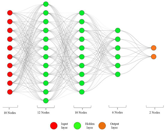
Figure 6.
ANN architecture in this study.
To assess and compare the efficacy of these algorithms, quantitative values and qualitative outcomes were used. Performance metrics such as the R-value and MSE were employed in this study. The training function for the ANN was the Levenberg–Marquardt algorithm. The stopping criteria included a gradient threshold of , a Mu value of , six validation checks, or a maximum of 1000 epochs, with the algorithm halting upon the first met condition.
Both RSA and IRSA algorithms comprised 100 populations and had a maximum of 1000 iterations. The coefficients for RSA were set at and , while for IRSA, the parameters were , , , , and . For the ANN, no specific boundary conditions were utilized since this algorithm relies on GD techniques to seek the optimal solution. This comprehensive methodology facilitated a thorough comparison and understanding of the strengths and limitations of each algorithm in the context of structural damage detection and quantification.
4.1. Single Damage
The convergence graph depicted in Figure 7 presents the regression line data, illustrating the convergence capabilities of each algorithm and displaying the R values of the trained network’s regression. All three algorithms achieved very high R values with the training set, all reaching an R value of one. Differences were only discernible when the network transitioned to the validation and test sets, where the aggregate R value for ANNIRSA was the highest at 1, surpassing ANNRSA’s 0.99999 and ANN’s lowest at 0.99998. All three networks exhibited high accuracy on the training data, leading to a close alignment of data points along the 45-degree regression line. Such an alignment indicated a strong correlation between the predicted outcomes and the target results across the training, validation, and testing datasets.
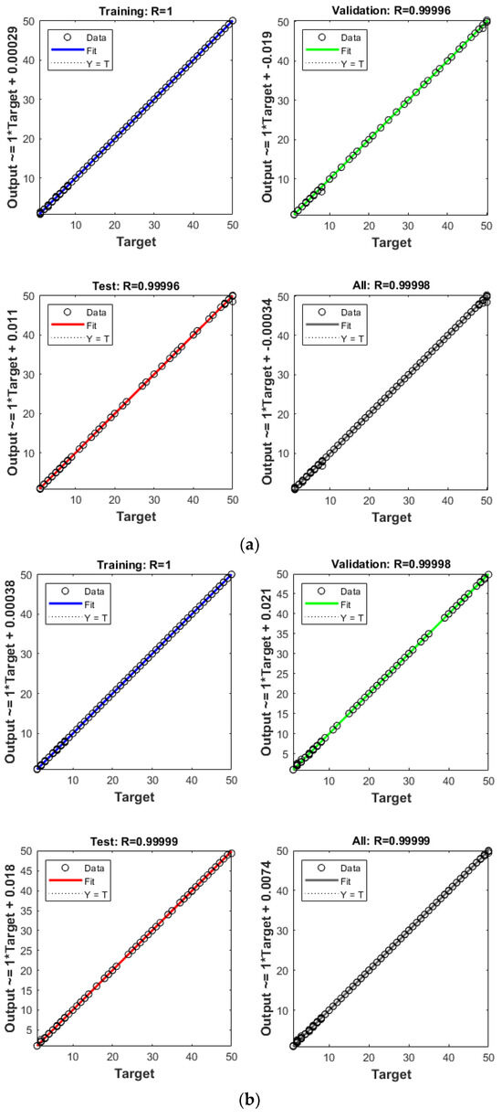
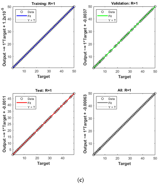
Figure 7.
Comparison of R values for (a) ANN, (b) ANNRSA, and (c) ANNIRSA.
Although the regression results for all algorithms are very promising, to truly gauge the effectiveness of the network training process, we considered the performance graph, which monitors the MSE and error distribution, with quantitative and qualitative results displayed in Figure 8. The findings indicate that the MSE calculated for ANNIRSA was the lowest, at 0.00033167, markedly superior to the MSE values for ANN and ANNRSA, which were 0.020569 and 0.0072929, respectively. This demonstrates that networks employing GD are prone to becoming trapped in local minima. In contrast, ANNRSA and ANNIRSA easily navigated out of local optima due to the RSA and IRSA algorithms being equipped with enhanced exploitation and search capabilities. Nonetheless, IRSA outperformed RSA by yielding lower MSE values when integrated with the ANN. This achievement is attributed to the implementation of adaptive and indices, as opposed to fixed values, enhancing the flexibility of the exploitation and search capabilities.
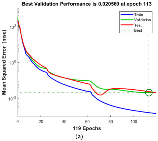
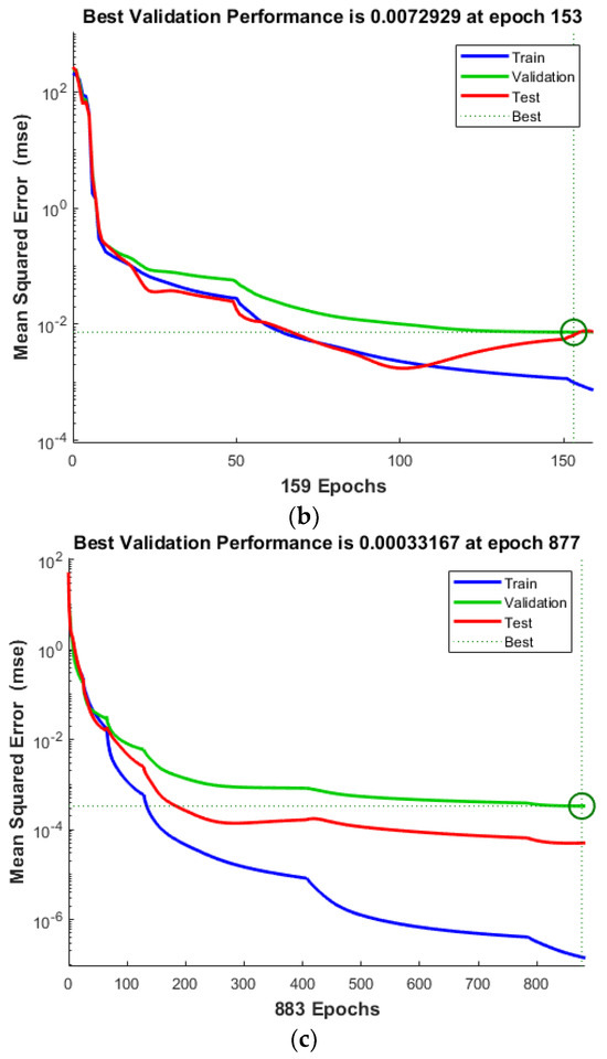
Figure 8.
Comparison of MSE values for single damage scenario of (a) ANN, (b) ANNRSA, and (c) ANNIRSA.
When examining the iteration counts at which the networks achieved optimal performance values, it is noted that ANN converged prematurely, halting after only 113 iterations, followed by ANNRSA at 153 iterations, and ANNIRSA extending to 877 iterations. This underscores ANNIRSA’s capability to evade local minima, as it consistently avoided triggering the initially set stopping conditions. Figure 9 elucidates the stopping condition encountered by the networks, specifically, the six times validation check. The green circles denote the beginning of the validation check condition. Also, the red diamons represent the time of validation check.
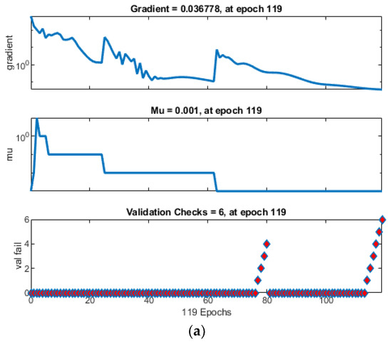
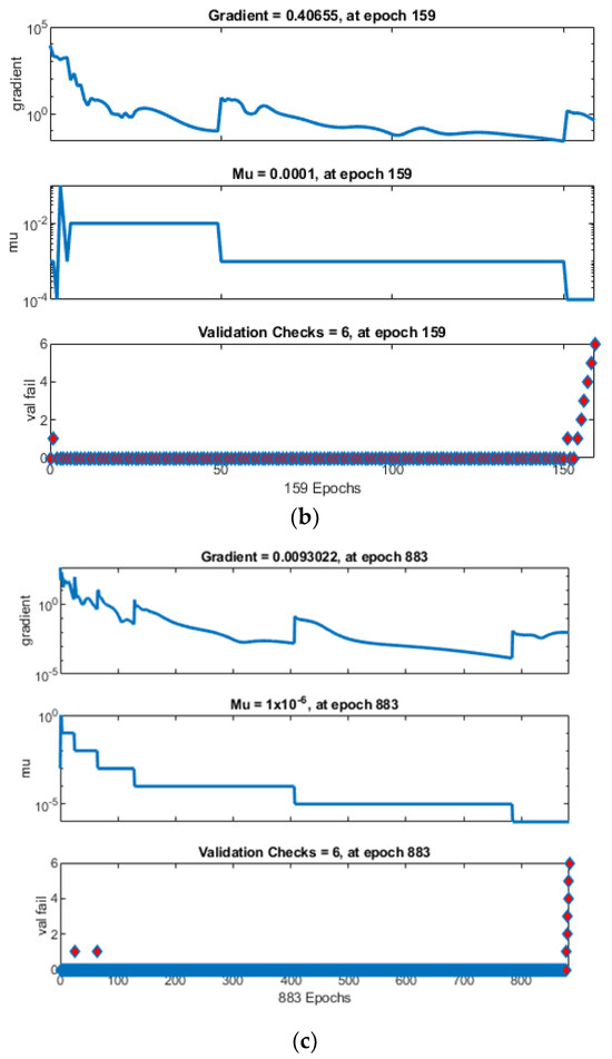
Figure 9.
Comparison of training state for (a) ANN, (b) ANNRSA, and (c) ANNIRSA.
Another perspective that elucidates why ANNIRSA excels can be observed in Figure 10, which depicts the error distribution of the networks. ANNIRSA demonstrates remarkable performance, with errors narrowly distributed, predominantly around the 0.001238 axis. Conversely, ANN exhibits the largest errors clustered around the −0.02105 area, while ANNRSA’s errors are around 0.01578.
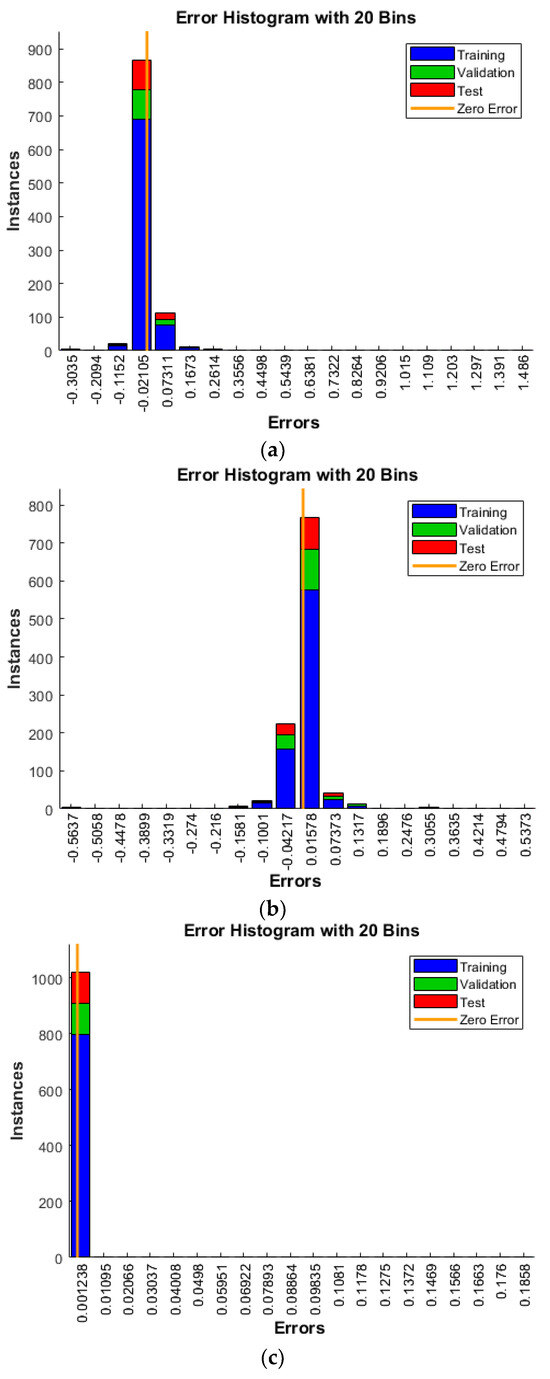
Figure 10.
Comparison of error values (another perspective) of (a) ANN, (b) ANNRSA, and (c) ANNIRSA.
Figure 11 presents a comparison chart between each network’s predicted values and their actual values. It is evident that the predictions made by ANN and ANNRSA closely follow the target line, yet some outliers distinctly deviate from the targets. In contrast, ANNIRSA performs impeccably, with all predicted values aligning precisely with the target values, indicating a perfect prediction.
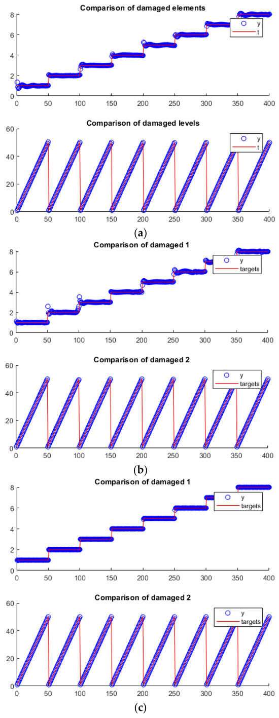
Figure 11.
Comparison of output targets for single damage scenario using (a) ANN, (b) ANNRSA, and (c) ANNIRSA.
4.2. Multiple Damage
The efficacy of ANNIRSA was assessed through the application of multielement damage scenarios with larger and more challenging datasets. Figure 12 illustrates the convergence capabilities of the ANN, ANNRSA, and ANNIRSA. Qualitatively, the data values for ANNIRSA can be observed to be closely distributed around the regression line, indicating superior convergence compared to ANN and ANNRSA, which exhibit more significant dispersion across the data series. The R values provide insight into the smoother convergence graph of ANNIRSA, which boasts an overall R value of 0.99879, significantly outstripping ANNRSA’s 0.99793 and ANN’s 0.99684.
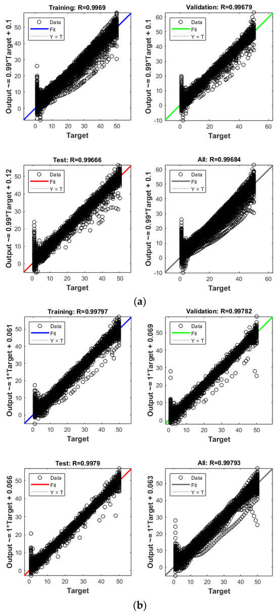
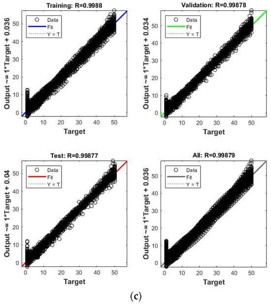
Figure 12.
Comparison of R values of (a) ANN, (b) ANNRSA, and (c) ANNIRSA.
The performance chart for the multielement damage scenarios reveals the robustness of ANNIRSA, which maintained performance consistently up to the stopping point of 1000 iterations. In contrast, ANN prematurely halted at 430 iterations with an MSE of 1.3969, and ANNRSA, though outperforming traditional ANN, ceased at 883 iterations with an MSE of 0.94197, both markedly inferior to ANNIRSA’s final MSE of 0.53333, as shown in Figure 13. This reaffirms the superiority of ANNIRSA, which adeptly escapes local minima to enhance algorithmic performance in both single- and multielement damage cases. Figure 14 indicates that ANN and ANNRSA stopped due to meeting the validation check condition of 6, whereas ANNIRSA only ceased upon reaching the 1000 iteration condition.
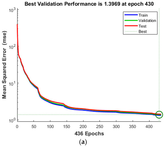
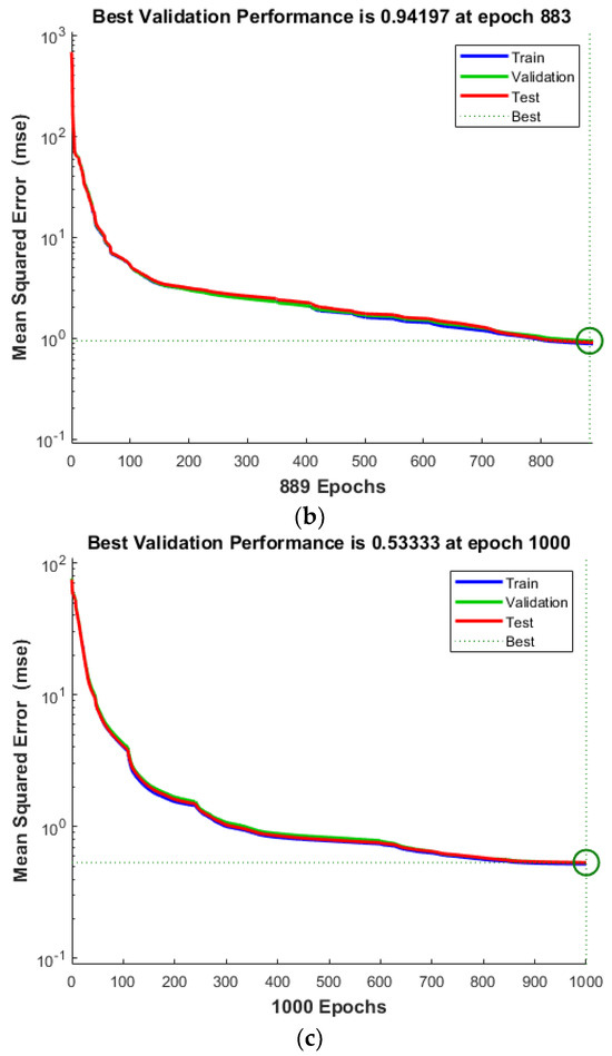
Figure 13.
Comparison of MSE values for multiple damage scenario of (a) ANN, (b) ANNRSA, and (c) ANNIRSA.
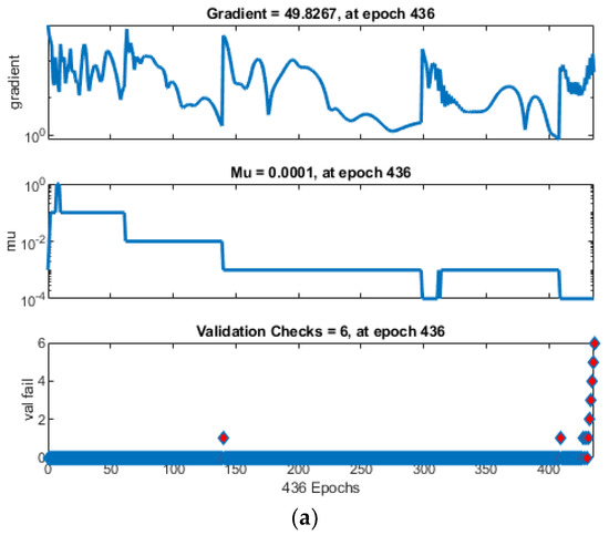
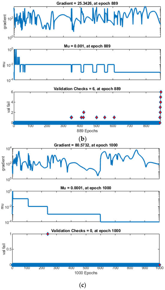
Figure 14.
Comparison of training state of (a) ANN, (b) ANNRSA, and (c) ANNIRSA.
Figure 15 displays the error distribution for the ANN, ANNRSA, and ANNIRSA. It demonstrates that all three networks yielded low error rates post-training and testing. Nonetheless, ANNIRSA registered an impressively low error distribution, narrowly centered around 0.1442, the smallest compared to ANN’s 0.6274 and ANNRSA’s 0.1548, further accentuating its dominance.
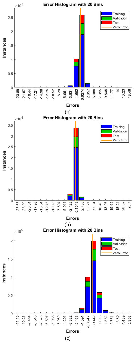
Figure 15.
Comparison of error values of (a) ANN, (b) ANNRSA, and (c) ANNIRSA.
Finally, the alignment of the networks’ actual and predicted values can be scrutinized in Figure 16. It is apparent that the multidamage problem was more complex than the single-damage scenario, as evidenced by all three charts, which showed less-than-perfect alignment between predictions and targets. Most notably, this misalignment was pronounced for the damaged elements, with numerous erroneous predictions across all charts. Yet, ANNIRSA still outperformed the others, exhibiting fewer inaccuracies and a more recognizable pattern of predicted and target data lines.
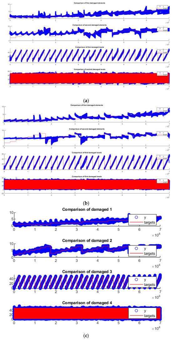
Figure 16.
Comparison of output targets for multiple damage scenario of (a) ANN, (b) ANNRSA, and (c) ANNIRSA.
5. Conclusions and Future Works
This research introduced an innovative approach that combines an ANN with a sophisticated optimization algorithm for structural damage detection. The key feature of this methodology is the incorporation of the RSA’s stochastic search capability, working in conjunction with GD techniques. This integration was designed to circumvent the issue of the network being trapped in local minima throughout its training phase. Consequently, an enhanced version of RSA was also introduced. The results demonstrated that the efficiency of ANNIRSA is significantly improved compared with that of the conventional ANN because the IRSA rectifies the local optima issues inherent in GD by introducing a suite of dynamic coefficients that amplify randomness and the likelihood of locating the optimal solution, as opposed to the static coefficients used in the original RSA. For assessing the effectiveness of ANNIRSA, a computational model of the Nam O Bridge was developed. A variety of scenarios derived from this model were utilized as datasets for both training and prediction purposes. Additionally, ANN and ANNRSA were implemented to provide a comparative framework. The analysis of the results led to the drawing of several important conclusions:
- All the algorithms evaluated—ANN, ANNRSA, and ANNIRSA—demonstrated proficiency in identifying structural damage. The R values for all scenarios surpassed 0.99, indicating high correlation, and the MSE values were notably low.
- The dependency of the ANN on GD techniques leads to a propensity to being trapped in local minima. This limitation manifests as inaccuracies in damage detection when the ANN is applied, especially in scenarios where the network architecture is intricate and beset with a multitude of local optima.
- IRSA proved its mettle by enhancing the ANN, bolstering accuracy in the damage detection using the numerical model.
- ANNIRSA effectively tackled the challenge of local minima typically encountered in traditional ANN models. Consequently, the proposed approach presents considerable potential for practical applications in solving real-world problems.
From these outcomes, future directions can be proposed as follows:
- Subsequent studies should apply this methodology in damage detection research on actual structures such as buildings, bridges, etc.
- IRSA can be implemented to optimize global search capabilities and improve the effectiveness of deep learning network models.
- Researchers can further develop and refine the IRSA algorithm by adjusting weights, incorporating search techniques like Levy flights, and strategically distributing operational groups to achieve greater efficiency.
Author Contributions
Conceptualization, N.D.B.; methodology, N.D.B., T.H.N. and M.D.; software, N.D.B. and M.D.; validation, N.D.B., T.H.N. and M.D.; formal analysis, N.D.B., T.H.N. and M.D.; investigation, T.H.N.; resources, N.D.B.; data curation, N.D.B.; writing—original draft preparation, N.D.B.; writing—review and editing, N.D.B. and T.H.N.; visualization, N.D.B.; supervision, N.D.B. and M.D. All authors have read and agreed to the published version of the manuscript.
Funding
This research was funded by University of Transport and Communications (UTC) under grant number T2022-CN-002TĐ.
Data Availability Statement
Data are contained within the article.
Conflicts of Interest
The authors declare no conflict of interest.
References
- Ngoc, L.N.; Huu, Q.N.; Ngoc, L.N.; Tran, H.N. Performance evaluation of the artificial hummingbird algorithm in the problem of structural damage identification. Transp. Commun. Sci. J. 2023, 74, 413–427. [Google Scholar] [CrossRef]
- Viet, L.H.; Thi, T.T.; Xuan, B.H. Swarm intelligence-based technique to enhance performance of ANN in structural damage detection. Transp. Commun. Sci. J. 2022, 73, 1–15. [Google Scholar] [CrossRef]
- Việt, H.H.; Anh, T.; Đức, T.P. Utilizing artificial neural networks to anticipate early-age thermal parameters in concrete piers. Transp. Commun. Sci. J. 2023, 74, 445–455. [Google Scholar] [CrossRef]
- Mohammadi, N.; Mirabedini, S.J. Comparison of Particle Swarm Optimization and Backpropagation Algorithms for Training Feedforward Neural Network. J. Math. Comput. Sci. 2014, 12, 113–123. [Google Scholar] [CrossRef]
- Hinton, G.E.; Srivastava, N.; Krizhevsky, A.; Sutskever, I.; Salakhutdinov, R.R. Improving neural networks by preventing co-adaptation of feature detectors. arXiv 2012, arXiv:1207.0580. [Google Scholar] [CrossRef]
- Prabowo, A.S.; Sihabuddin, A.; Sn, A. Adaptive Moment Estimation on Deep Belief Network for Rupiah Currency Forecasting. Indones. J. Comput. Cybern. Syst. 2019, 13, 31–42. [Google Scholar] [CrossRef][Green Version]
- Wang, R.-L.; Guo, S.-S.; Okazaki, K. A hill-jump algorithm of Hopfield neural network for shortest path problem in communication network. Soft Comput. 2009, 13, 551–558. [Google Scholar] [CrossRef]
- Sathasivam, S.; Alzaeemi, S.A.; Velavan, M. Mean-Field Theory in Hopfield Neural Network for Doing 2 Satisfiability Logic Programming. IJMECS 2020, 12, 27–39. [Google Scholar] [CrossRef]
- Ojha, V.K.; Abraham, A.; Snášel, V. Metaheuristic design of feedforward neural networks: A review of two decades of research. Eng. Appl. Artif. Intell. 2017, 60, 97–116. [Google Scholar] [CrossRef]
- Fei, X.; Shuotao, H.; Hao, Z.; Daogang, P. A Comparative Research on Condenser Fault Diagnosis Based on Three Different Algorithms. TOEEJ 2014, 8, 183–189. [Google Scholar] [CrossRef][Green Version]
- Chagas, S.H.; Martins, J.B.; de Oliveira, L.L. An approach to localization scheme of wireless sensor networks based on artificial neural networks and Genetic Algorithms. In Proceedings of the 10th IEEE International NEWCAS Conference, Montreal, QC, Canada, 17–20 June 2012; IEEE: Piscataway, NJ, USA, 2012; pp. 137–140. [Google Scholar] [CrossRef]
- Tran-Ngoc, H.; Khatir, S.; Le-Xuan, T.; Tran-Viet, H.; De Roeck, G.; Bui-Tien, T.; Wahab, M.A. Damage assessment in structures using artificial neural network working and a hybrid stochastic optimization. Sci. Rep. 2022, 12, 4958. [Google Scholar] [CrossRef] [PubMed]
- Kumar, N.; Kumar, D. An Improved Grey Wolf Optimization-Based Learning of Artificial Neural Network for Medical Data Classification. J. Inf. Commun. Technol. 2021, 20, 213–248. [Google Scholar] [CrossRef]
- Ban, H.G. Variable neighbourhood search-based algorithm to solve the minimum back-walk-free latency problem. IJCAT 2021, 65, 55. [Google Scholar] [CrossRef]
- Abualigah, L.; Abd Elaziz, M.; Sumari, P.; Geem, Z.W.; Gandomi, A.H. Reptile Search Algorithm (RSA): A nature-inspired meta-heuristic optimizer. Expert Syst. Appl. 2022, 191, 116158. [Google Scholar] [CrossRef]
- Shirazi, M.I.; Khatir, S.; Benaissa, B.; Mirjalili, S.; Wahab, M.A. Damage assessment in laminated composite plates using modal Strain Energy and YUKI-ANN algorithm. Compos. Struct. 2023, 303, 116272. [Google Scholar] [CrossRef]
- Khatir, S.; Tiachacht, S.; Thanh, C.-L.; Bui, T.Q.; Wahab, M.A. Damage assessment in composite laminates using ANN-PSO-IGA and Cornwell indicator. Compos. Struct. 2019, 230, 111509. [Google Scholar] [CrossRef]
- Tran-Ngoc, H.; Khatir, S.; De Roeck, G.; Bui-Tien, T.; Nguyen-Ngoc, L.; Abdel Wahab, M. Model updating for Nam O bridge using particle swarm optimization algorithm and genetic algorithm. Sensors 2018, 18, 4131. [Google Scholar] [CrossRef] [PubMed]
- François, S.; Schevenels, M.; Dooms, D.; Jansen, M.; Wambacq, J.; Lombaert, G.; Degrande, G.; De Roeck, G. Stabil: An educational Matlab toolbox for static and dynamic structural analysis. Comput. Appl. Eng. Educ. 2021, 29, 1372–1389. [Google Scholar] [CrossRef]


Disclaimer/Publisher’s Note: The statements, opinions and data contained in all publications are solely those of the individual author(s) and contributor(s) and not of MDPI and/or the editor(s). MDPI and/or the editor(s) disclaim responsibility for any injury to people or property resulting from any ideas, methods, instructions or products referred to in the content. |
© 2024 by the authors. Licensee MDPI, Basel, Switzerland. This article is an open access article distributed under the terms and conditions of the Creative Commons Attribution (CC BY) license (https://creativecommons.org/licenses/by/4.0/).