Abstract
Adversarial sample-based privacy protection has its own advantages compared to traditional privacy protections. Previous adversarial sample privacy protections have mostly been centralized or have not considered the issue of hardware device limitations when conducting privacy protection, especially on the user’s local device. This work attempts to reduce the requirements of adversarial sample privacy protections on devices, making the privacy protection more locally friendly. Adversarial sample-based privacy protections rely on deep learning models, which generally have a large number of parameters, posing challenges for deployment. Fortunately, the model structural pruning technique has been proposed, which can be employed to reduce the parameter count of deep learning models. Based on the model pruning technique Depgraph and existing adversarial sample privacy protections AttriGuard and MemGuard, we design two structural pruning-based adversarial sample privacy protections, in which the user obtains the perturbed data through the pruned deep learning model. Extensive experiments are conducted on four datasets, and the results demonstrate the effectiveness of our adversarial sample privacy protection based on structural pruning.
1. Introduction
In recent years, deep learning models have received extensive research and application. Deep learning has effectively improved productivity and, to some extent, promoted societal development. However, science and technology are double-edged swords, and the automated inference of deep learning has posed unprecedented challenges to the personal privacy of Internet users.
Adversarial samples, as a weakness of deep learning, have been proposed [1]. By adding small perturbations to the input of a pre-trained deep learning model, it is easy to cause misclassification, and these inputs with added noise are referred to as adversarial samples. The existence of adversarial samples has had a significant impact on the practical application of deep learning and has become an important metric for evaluating the robustness of deep learning models.
However, in the field of data privacy protection, the emergence of adversarial samples could present a new opportunity for privacy protection techniques. Adversarial samples can cause misclassification in deep learning models, and if they can achieve misclassification specifically for sensitive attributes, they can protect the privacy of the underlying data. Now, there exist several approaches that utilize adversarial samples for privacy protection, including [2,3,4], and so on. In [2], inspired by [5], adversarial samples are generated by modifying the most influential elements of the input to achieve privacy attribute protection. Ref. [3] is a defense strategy against membership inference attacks [6], drawing inspiration from [7]. It employs multi-step gradients to generate adversarial samples and incorporates the magnitude of noise into the loss function, striking a balance between input utility and security.
Compared to traditional differential privacy [8], optimization-based approaches [9], and heuristic algorithms [10], it has been demonstrated that some adversarial sample-based privacy protections achieve better balance in terms of computational complexity, security, and data utility [2,3,4], making them more effective for privacy protection to some extent. Despite their own weaknesses, such as the attacks in [11], these approaches are still capable of altering the designs to enhance robustness. Privacy protections based on adversarial samples have their own advantages and can demonstrate their effectiveness in certain domains.
Inspired by the local differential privacy algorithm [12], we consider the question of whether privacy protection based on adversarial samples can be applied locally to better serve its privacy protection function. The greatest advantage of local differential privacy is that it does not require a trusted third party. We refer to the privacy protection based on adversarial samples deployed locally on the user’s device as the local adversarial sample privacy protection (LASPP).
Although [2] mentions that the defender can be software or browser plug-ins deployed on the user side, which may suggest a local solution without the need for additional local solutions, a closer examination of the process reveals that the model has a large number of parameters, making it difficult for users with poor devices to deploy locally. This issue was not considered in [2]. Although the model can be placed on a cloud device and called by local users, the non-trusted third parties who fully understand the defense model may still be able to gain access to users’ private information through backdoors. In addition, calling cloud devices locally will also bring about communication overhead and security issues. This paper prunes the deep learning model first and then distributes it to users locally, adding noise locally to reduce the threshold for users to use the model.
For [3], the defender itself is the model provider or the trusted third party. Hence, [3] is more likely to lean towards central deployment rather than on user devices. Deploying the defense locally on the user side can weaken the assumption that the defender is a trusted third party. However, user devices are limited, and deploying centralized models locally still faces challenges in making the models locally friendly. Therefore, this paper’s solution has a certain promoting effect on deploying LASPP locally on users’ devices. Furthermore, even in a centralized deployment of adversarial sample privacy protection solutions, the more lightweight ML model is more environmentally friendly.
Unlike the local differential privacy algorithm, the privacy protection based on adversarial samples requires a deep learning model, and generally, deep learning models have a large number of parameters, which poses a significant challenge for the LASPP. For example, in [2], the number of parameters in defending deep learning models exceeds , such a large parameter size will inevitably impose a significant burden on user devices. The limited computational capabilities of users’ local devices may be the biggest challenge in applying adversarial sample privacy protections locally at present. Fortunately, model pruning techniques [13,14,15,16,17,18,19,20,21,22,23,24] may bring new possibilities for the LASPP. Model pruning is a technique used to reduce the size and complexity of deep learning models. Through model pruning, unnecessary parameters, connections, and layers can be removed from the model, reducing the storage requirements of the model, accelerating inference speed, and reducing the consumption of computing resources.
Mainstream model pruning techniques can be broadly categorized into structural pruning [13,14,15,16,17,18,19,20,21] and non-structural pruning [22,23,24]. Structural pruning is a pruning technique based on the model’s structure. It reduces the size and complexity of the model by removing entire neurons, layers, or modules from the model. In non-structural pruning, thresholding is used to zero out or remove the parameters with smaller absolute values, resulting in a reduction in the number of parameters in the model. Non-structural pruning can significantly reduce the size and complexity of the model without altering its structure. Compared to non-structural pruning, structural pruning does not rely on specific AI accelerators or software to reduce memory overhead and computational costs, making it more widely applicable in practice [25,26].
The model pruning technique used in this article is structural pruning, mainly based on reference [15], which proposes using dependency graphs to enable structural pruning of any neural network. In this work, we apply the structural pruning technique to [2,3] to derive two privacy protections for adversarial samples based on the pruned model. We refer to these two privacy protections as structural pruning-based adversarial sample privacy protections (SP-ASPPs). Unlike [2,3], our scheme attempts to generate adversarial noise on the pruned model. As the pruned model has fewer parameters, it has the potential to be placed on the user side. To clearly illustrate our scheme, we illustrate our SP-ASPP in Figure 1. Through our attempt in this paper, we hope to provide some inspiration for future LASPPs.
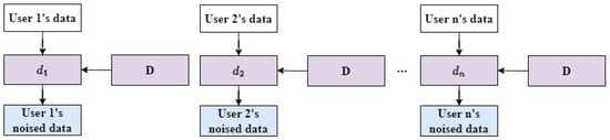
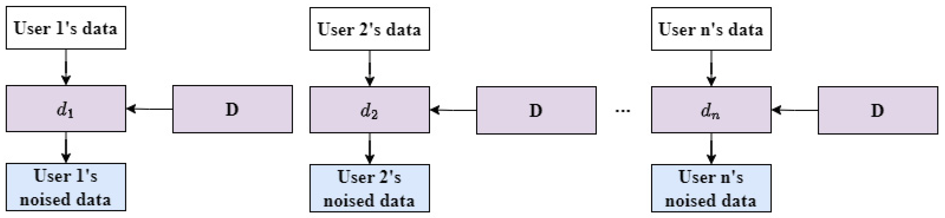
Figure 1.
The privacy protection based on adversarial samples requires a deep learning model. In this paper, the model pruning technique is employed to prune the deep learning model D and obtain the pruned model d. The pruned model d is then used to generate adversarial noise. Through the pruning process, the threshold for using adversarial sample privacy protection is reduced, making it easier to deploy adversarial sample privacy protection locally and thus achieve better privacy protection.
We adopt four datasets to validate the SP-ASPPs. Building upon references [2,3], we have designed a lightweight adversarial sample-based privacy protection scheme for this paper. To demonstrate the effectiveness of our approach, we need to compare it with the original scheme. Therefore, the four datasets chosen in this paper are exactly the same as those used in [2,3]. The first dataset is used to validate the first SP-ASPP. The subsequent three datasets are used to validate the second SP-ASPP. The first dataset is derived from [2], while the subsequent three datasets are derived from [3].
We evaluate our SP-ASPP scheme by subjecting it to the attacks used in [2,3]. We compare our SP-ASPPs with [2,3] separately. For the same dataset, our first SP-ASPP uses the same attack model as [2], and our second SP-ASPP uses the same attack model as [3]. The inference accuracy of the attack model represents the effectiveness of the defense scheme, where a higher accuracy indicates a weaker defense effect, and vice versa. With the reduction in ML model parameters, if the decrease in defense model accuracy is minimal and the increase in attack model inference accuracy is also minimal, it demonstrates the effectiveness of the proposed SP-ASPPs in this paper.
The effectiveness of our approach is demonstrated by comparing the accuracy, size, and effectiveness of noising before and after pruning the defense model. The impact of noising is measured by the inference accuracy of the attack model. Thorough experiments demonstrate the effectiveness of our SP-ASPPs. The contributions of this article include the following.
- To our best knowledge, our research is one of the early considerations in weakening the contradiction between limited user device capabilities and a large number of parameters of deep learning models in privacy protection via adversarial samples.
- We use state-of-the-art model pruning techniques and combine them with advanced adversarial sample privacy protections to design two structural pruning-based adversarial sample privacy protections and verify their effectiveness.
- Thorough experiments on four real-world datasets demonstrate that the performance of the defense model after pruning is not significantly affected and prove the feasibility of the proposed locally-based privacy protection for adversarial samples.
The remaining parts of this paper are organized as follows. In Section 2, we discuss the related work. In Section 3, we introduce the participants and define the key issues of our work. In Section 4, we propose the pruning principle and our two structural pruning-based adversarial sample privacy protections. In Section 5, we describe our experimental setup, and provide the experimental results to validate the effectiveness of our work. Finally, in Section 6, we conclude our work.
2. Related Work
This section mainly introduces the related work of this paper, which mainly includes two aspects closely related to this paper. One is the privacy protection scheme based on adversarial samples, which forms the basis of this paper. The other is the related work on model structure pruning, which is the source of the pruning algorithm in this paper.
2.1. Privacy Protection Based on Adversarial Samples
Jia et al. [2] proposed a defense against attribute inference attack, which consists of two stages: noise generation and noise injection. In the noise generation stage, they draw inspiration from [5] and consider both the elements that have the most significant impact on the output and the degree to which these elements can be altered. They modify the elements that have a significant impact and can be changed substantially, iteratively altering one element at a time until the desired output is achieved and then stop the iteration and output the noised data that satisfies the requirements. In the second stage, random noise is added to make the inference of the attack model resemble random guessing.
Jia et al. [3] proposed a defense against membership inference attack, which consists of two stages: noise generation and noise injection. In the noise generation stage, they draw inspiration from multi-step adversarial sample generation methods [7]. However, their loss function takes into account three elements. The first element ensures that the attack model’s binary classifier cannot obtain useful information. The second element ensures that the output label of the target model remains unchanged. The third element ensures that the magnitude of the noise is as small as possible. The noisy data are generated through multiple iterative steps. In the second step, random noise is added to prevent the attacker from inferring the added noise through the output.
Shao et al. [4] utilized adversarial samples to protect the text-based CAPTCHA. Their scheme consists of two stages: In the first stage, they construct foreground and background using randomly sampled fonts and background images and then combine them to create recognizable pseudo-adversarial CAPTCHA images. In the second stage, they design and apply a highly transferable text CAPTCHA adversarial attack method to better impede CAPTCHA solvers.
Li et al. [27] proposed a face image de-identification scheme, which includes four stages: face feature evaluation, privacy-oriented face obfuscation, targeted natural image synthesis, and adversarial perturbation. Their scheme demonstrates that adversarial samples can be used in the domain of face image de-identification.
Salman et al. [28] proposed PhotoGuard, which employs adversarial examples to protect users’ private photos from malicious editing by large diffusion models. Two privacy protection mechanisms, Encoder attack and Diffusion attack, are developed for the encoder and the entire large diffusion model.
Shan et al. [29] proposed Glaze, a solution that adds imperceptible noise to images to prevent large models from learning their style, thus protecting the copyright of artists.
The above are all privacy protections based on adversarial samples. Although they have considered the security of the model and the availability of data, and have demonstrated that their solution achieves a good balance between security and usability, they have not taken into account the limitations of users’ local devices and their knowledge. Knowledge limitations may arise because users may not be professional data security workers and may be unfamiliar with certain operations. In this paper, we have explored some issues that were not considered in previous research, with the expectation that our study can contribute to advancing the development of LASPP to a certain extent.
2.2. Model Pruning
Model pruning techniques can be divided into two categories: structural pruning and non-structural pruning. In this paper, we are solely concerned with structured pruning techniques.
Inspired by the linear properties of convolutions, Ding et al. [13] attempted to make filters gradually approach each other and eventually become identical to achieve network slimming. To this end, they proposed a new optimization method called centripetal SGD (C-SGD), which can train multiple filters to converge to a point in the parameter space. When training is complete, removing the identical filters can prune the network without causing performance loss, thus eliminating the need for fine-tuning.
You et al. [14] introduced a global filter pruning algorithm that transforms the output of a conventional CNN module by multiplying it with channel-wise scaling factors (i.e., gates). Setting the scaling factor to zero is equivalent to removing the corresponding filter. They utilized the Taylor expansion to estimate the change in the loss function when setting the scaling factor to zero and used the estimation to rank the global importance of filters. Subsequently, they pruned the network by removing unimportant filters. After pruning, all scaling factors were merged back into the original module, eliminating the need for introducing special operations or structures. Additionally, they introduced an iterative pruning framework called Tick-Tock to improve the accuracy of pruning. Extensive experiments demonstrated the effectiveness of their approach.
Shen et al. [16] combined the benefits of post-training pruning and pre-training pruning to propose a method that performs early pruning during training without compromising performance. Instead of pruning at initialization, this method quickly determines the model structure using a few rounds of training, evaluates the importance ranking of the main subnetworks, and then triggers pruning to ensure model stability and achieve early pruning during the training process.
Gao et al. [17] proposed a novel channel pruning method to reduce the computational and storage costs of convolutional neural networks. The target subnetwork is learned during model training and then used to guide the learning of model weights via partial regularization. The target subnetwork is learned and generated using an architecture generator, which can be effectively optimized. In addition, they also derived the proximal gradient for their proposed partial regularization to facilitate the structural alignment process. By these designs, the gap between the pruned model and the subnetwork is reduced, which improves pruning performance.
Shen et al. [18] proposed hardware-aware latency pruning, which formalizes structured pruning techniques as a resource allocation optimization problem aimed at maximizing accuracy while constraining latency within a budget on the target device. They ultimately solved the optimization problem using an enhanced knapsack problem solver, and this approach has been demonstrated to surpass previous work in achieving a balance between accuracy and efficiency.
Fang et al. [19] proposed a pruning scheme for large diffusion models, called Diff-Pruning, with the aim of learning lightweight diffusion models from existing models without extensive retraining. The essence of Diff-Pruning is encapsulated in a Taylor expansion over pruned timesteps, a process that disregards non-contributory diffusion steps and ensembles informative gradients to identify important weights.
Hou et al. [20] proposed a simple yet effective channel pruning technique, called pruning via resource reallocation (PEEL), to rapidly generate pruned models with negligible cost. Specifically, PEEL first constructs a predefined backbone and then conducts resource reallocation on it to shift parameters from less informative layers to more important layers in one round, thus amplifying the positive effect of these informative layers.
Ma et al. [21] addressed the compression problem of large language models (LLMs) within two constraints: task-agnosticism and minimizing reliance on the original training dataset. Their method, called LLM-Pruner, utilizes structured pruning techniques to selectively remove non-critical coupling structures based on gradient information while preserving a significant portion of the functionality of LLMs. To achieve this, with the help of the LoRA technique, the performance of the pruned model can be effectively restored in just 3 h with only 50 K data.
Fang et al. [15] investigated a highly challenging yet rarely explored task of general structure pruning for any architecture such as CNNs, RNNs, GNNs, and Transformers. The most prominent obstacle to achieving this goal is structural coupling, which not only forces different layers to be pruned simultaneously but also expects all deleted parameters to be always unimportant, avoiding structural issues and significant performance degradation after pruning. To address this issue, they proposed a generic fully automated method—DepGraph, which explicitly models the dependency relationships between layers and comprehensively groups coupled parameters for pruning. They extensively evaluated their method on several architectures and tasks, including ResNe(X)t, DenseNet, MobileNet, and Vision Transformer for images, GAT for graphs, DGCNN for 3D point clouds, and LSTM for language, and demonstrated that the proposed method consistently yields satisfactory performance even using simple norm-based criteria.
There exist many types of model pruning techniques, including those targeted at convolutional models and large diffusion models. In fact, these model pruning techniques can be applied to reduce the size of deep models. We ultimately chose [15] as our pruning scheme mainly because it demonstrated strong applicability and showed promising performance in their paper. However, other pruning schemes could also be explored, and this remains future work.
3. Model Preparation
This section mainly introduces the preparatory work for the lightweight adversarial sample privacy protection scheme, discussing the potential participants in the lightweight adversarial sample privacy protection scheme including three parties: defender, user, and attacker. In order to effectively propose a lightweight adversarial sample privacy protection scheme, three definitions are put forward to ensure the effectiveness of the model: the first one ensures that there is little change in the accuracy of the defense model before and after model pruning, the second guarantees a certain pruning ratio, and the third ensures the defensive effect of noise on the pruned model. Generally speaking, the first definition forms the basis for satisfying the second and third definitions.
3.1. Participating Parties
3.1.1. Defender
The defender designs and trains the defense model and distributes the obtained defense model to users assuming that the defender designs a larger model, denoted as D. To meet the diverse hardware requirements of users, assume that the defender can compress the model and control the pruning ratio, resulting in multiple pruned defense models . After obtaining the pruned models, the defender further trains each model and finally distributes them to the user. One key operation that the defender needs to perform during this process is:
where the long arrow in Formula (1) represents the structural pruning operation. To facilitate the comparison of results, the defender also generated adversarial noise data using the unpruned defense model. We denote the data to which the noise is added as . This process can be expressed as follows:
where the long arrow in Formula (2) represents the defender’s adversarial noise injection process.
3.1.2. User
For each user, distinguished by a subscript i, . N represents the number of users. Firstly, user i has their own data , which is a vector or matrix of a certain dimension that needs to be compatible with the defense models distributed by the defender. Based on the defense models, the user can generate adversarial samples and obtain a noisy vector . This process can be expressed as follows:
where the long arrow in Formula (3) represents the local perturbation process of user i.
3.1.3. Attacker
The attacker can train an attack model A to infer the noisy data. The information acquired by the attack model on is defined as .
3.2. Problem Definition
We use to represent the number of model parameters. In order to ensure that the pruned model maintains high accuracy, has a small parameter scale, and local noise addition is effective, we provide the following three definitions.
Definition 1.
Before and after model pruning, the models are represented as D and d, with their accuracy on the test set denoted as and , respectively. If the model d has certain effects, there exists a small positive number such that .
Definition 2.
Before and after model pruning, the models are represented as D and d, with their parameter sizes denoted as and , respectively. If the model parameters of d are small enough to satisfy a certain condition, then there exists a positive number r such that .
Definition 3.
Before and after model pruning, the models are represented as D and d, with the obtained adversarial noisy data being and , respectively. For any attack model, its inference accuracy on is represented as , and its inference accuracy on is represented as . To ensure the effectiveness of the model pruning privacy protection, there exist two small positive numbers q and n such that and .
4. The Proposed Scheme
This section mainly introduces the model pruning algorithm adopted in this paper, the first adversarial sample privacy protection scheme based on structural pruning, and the second adversarial sample privacy protection scheme based on structural pruning.
4.1. Model Pruning
The model pruning technique used in this study is referenced from [15], which involves dependency graph, grouping, and importance assessment. For ease of reference in the subsequent discussion, we denote this pruning process as , where D represents the defense model and d represents the pruned defense model.
4.1.1. Dependency Graph and Grouping
The neural network is represented as , which is decomposed into finer and fundamental components, i.e., . Here, each component f represents a parameterized layer such as convolution or a non-parameterized operation such as residual addition. The input and output of component are denoted as and , respectively. Thus, for any network, the final decomposition becomes . The network can be redefined as follows:
where the symbol ↔ represents the connection between two adjacent layers, and L represents the total number of layers. This leads to the existence of inter-layer dependency and intra-layer dependency. Inter-layer dependency exists in the connected layers , denoted as . Intra-layer dependency exists when and have the same pruning scheme, represented as , denoted as . Based on the above symbols, the dependency model is constructed as follows:
where the symbols ∨ and ∧ represent logical and logical , respectively. The function is an indicator function that returns if the connection exists. Based on the above dependency graph, the components are divided into multiple groups, where there is no dependency relationship between each group, but there is a dependency relationship within each group.
4.1.2. Importance Evaluation
We assume there is a group under -norm, where the importance of each parameter is defined as for each parameter in group g. The importance of group g used in this article is defined as . The survival of each group is determined according to their importance ranking.
4.2. The First SP-ASPP
We designed our privacy protection based on reference [2]. However, unlike [2], our scheme involves users performing the noise injection process themselves and uploading the perturbed data to the server, while attackers collect the user’s perturbed data for final inference. Similar to [2], the first SP-ASPP consists of two phases: the noise generation phase and the random noise injection phase.
In the noise generation phase, the machine learning model is primarily pruned. The pruned model is then distributed to each user. Upon receiving the pruned and trained model, each user starts adding noise to their own data. For simplicity, this paper does not consider communication overhead and assumes that the defender performs model pruning and training tasks. Unlike [2], we assume that users have all the necessary permissions for modifying and adding privacy, which is reasonable locally since users have the most authority over their own data.
The algorithm is presented in Algorithm 1. The variable denotes the maximum number of iterations for generating adversarial noise, which is determined by user i and can be different for each user. The term in the algorithm represents a random selection mechanism that chooses perturbed data with a probability of . The calculation of is obtained by solving the following optimization problem:
where represents the probability distribution that user i wants the output to satisfy, is the optimal probability obtained by user i, and is the noise amplitude set by user i with . The optimization problem above is solved by user i. “” refers to the Kullback–Leibler divergence [30]. The theoretical solution to the above optimization problem can be found in [2], and can be directly used to obtain .
| Algorithm 1 The first SP-ASPP |
Input: Number of users N, data of the ith user , dimension of K, defense model D, minimum perturbation magnitude . Output: .
|
4.3. The Second SP-ASPP
We have designed a second structural pruning-based adversarial sample privacy protection based on [3]. The key difference is that users perform the noise generation process locally and then upload it to the server. This privacy protection also consists of two stages: noise generation stage and random noise addition stage. In the noise generation stage, the defender needs to train the defense model D and then perform pruning. The pruned model undergoes secondary training to obtain d. During this process, the defender needs to ensure that the model accuracy satisfies Definition 1. After receiving d, the user applies noise to the logits vector obtained from the target model, resulting in the noisy data.
We present the entire process in Algorithm 2. For the sake of uniformity, is used to represent the data to be noised, and is used to represent the noised data. The activation function of the output layer of the pruned defense model d is a sigmoid function, and the structure before the activation function is represented as h. Thus, the loss L can be expressed as:
where the values of and are chosen by the user i. , , and are constants that can be selected by the user. refers to the one-time randomness mentioned in [3]. When sampling noise data, the user employs one-time randomness to ensure that they always return the same noised data for the same data sample.
| Algorithm 2 The second SP-ASPP |
Input: Number of users N, data of the ith user , defense model D. Output: .
|
5. Experiment
This section mainly introduces the experiments conducted in this paper, including the experimental setup and results. The setup section mainly covers the datasets used in the paper and the detailed configurations of the two SP-ASPPs. The results section presents the experimental results of the two SP-ASPPs.
5.1. Experimental Settings
5.1.1. Datasets
The used dataset consists of four parts, with the first dataset sourced from [2] and the following three datasets sourced from [3]. For distinction, the first dataset is referred to as “Att”. Here, only a brief introduction to the datasets is provided, while specific usage instructions can be found in [2,3].
Att. This dataset can be obtained from GitHub ( https://github.com/jinyuan-jia/~AttriGuard (accessed on 25 November 2023)). The dataset comprises 16,238 samples, with each sample consisting of 10,000 features. Each feature represents a user’s rating for a specific app, and the rating values are normalized to 0, 0.2, 0.4, 0.6, 0.8, and 1.0. If a feature is missing, it is replaced with 0. The privacy attribute pertains to the user’s city of residence or past residence, encompassing a total of 25 cities.
Location. This dataset can be obtained from GitHub (https://github.com/privacytrustlab/datasets/dataset_location.tgz (accessed on 25 November 2023)). This dataset contains 5010 samples, each with 446 binary features representing whether the user has visited a certain location or not. The samples are categorized into 30 classes.
Texas100. This dataset can be obtained from GitHub (https://github.com/privacytrustlab/datasets/dataset_texas.tgz (accessed on 25 November 2023)). This dataset comprises 67,330 samples, each with 6170 binary features representing external causes of injury, diagnosis, patient procedures, and general information. These samples are divided into 30 classes, with each class representing a common disease.
CH-MNIST. This dataset can be obtained from Kaggle (https://www.kaggle.com/kmader/colorectal-histologymnist (accessed on 25 November 2023)). This dataset contains tissue slice image data of colon cancer patients, with each image having dimensions of . There are a total of 5000 samples in this dataset, which are divided into eight classes.
5.1.2. The First SP-ASPP
The experimental settings include the defense model, the attack model, and the other settings.
The defense model. The defense model is trained by the defender. The structure of the defense model consists of a three-layer fully connected neural network with neuron counts of 10,000, 40,000, and 25, respectively. The activation function used in the middle layer is ReLU, while the output layer uses the softmax activation function. There is a dropout layer between the second and third layers, with a dropout rate of 0.7. The optimizer used is Adam, and the loss function is cross-entropy. The learning rate is set to 0.0005, and each training batch contains 200 samples. The training is performed for 100 epochs.
The pruned defense model is also trained by the defender. The only modification made is changing the neuron count in the middle layer while keeping the input and output layer neuron counts unchanged. A speed-up factor is introduced, defined as speed-up = (Base MACs)/(Pruned MACs), where MAC represents multiply–accumulate operations. In the experiments, the speed-up factor is set to 2, 4, 6, …, 200 to observe the effect of different speed-up factors on the final noise addition. A speed-up factor of 1 corresponds to no pruning, and larger speed-up factors indicate higher pruning ratios. After pruning the defense model, it is further trained with parameters similar to those before pruning.
The attack model. To verify the defense effectiveness of the model, an attack model is also trained. The structure of the attack model consists of a three-layer fully connected neural network with neuron counts of 10,000, 30,000, and 25, respectively. The activation function used in the middle layer is ReLU, while the output layer uses the softmax activation function. There is a dropout layer between the second and third layers, with a dropout rate of 0.7. The optimizer used is SGD, and the loss function is cross-entropy. The learning rate is set to 0.05, and each training batch contains 100 samples. The training is performed for 50 epochs.
The purpose of training the attack model is to evaluate the defense effectiveness of the defense model by measuring its ability to resist attacks launched by the attack model.
The other setting. User i in the noise generation process has multiple options for the selection of . In this paper, the selected represents the proportion of users from the training set residing in the 25 cities. The value of is set to 1.5. In Algorithm 1, , , , , and .
5.1.3. The Second SP-ASPP
The experimental settings include the defense model, the attack model, and the other settings.
The defense model. The second local privacy protection is mainly validated using the last three datasets. The defense models are all fully connected neural networks, and for the three datasets, the intermediate and output layers are the same, consisting of . The input dimensions for Location, Texas100, and CH-MNIST are 30, 100, and 8, respectively. The activation function between layers is , and the activation function for the output layer is . The defender compresses the defense model and then re-trains it. Throughout the process, the SGD optimizer is used, as well as binary cross-entropy loss, a learning rate of 0.01, and a batch size of 64. The number of training epochs for the defense model before and after compression is 400 and 100, respectively.
The attack model. The attack model is a fully connected neural network, and for the three datasets, the intermediate and output layers are the same, consisting of . The input dimensions for Location, Texas100, and CH-MNIST are 30, 100, and 8, respectively. The activation function between layers is , and the activation function for the output layer is . The SGD optimizer is used, as well as binary cross-entropy loss, a learning rate of 0.01, and a batch size of 64. The number of training epochs for the attack model is 400.
The other setting. For Location, Texas100, and CH-MNIST, N is 2000, 20,000, and 2000, respectively. , , , , and the initial value of is set to 0.1.
5.2. Experimental Results
5.2.1. The First SP-ASPP
We evaluate the first SP-ASPP from three aspects: defense model accuracy, model size, and attack inference accuracy, corresponding to Definitions 1–3 in the previous section, respectively.
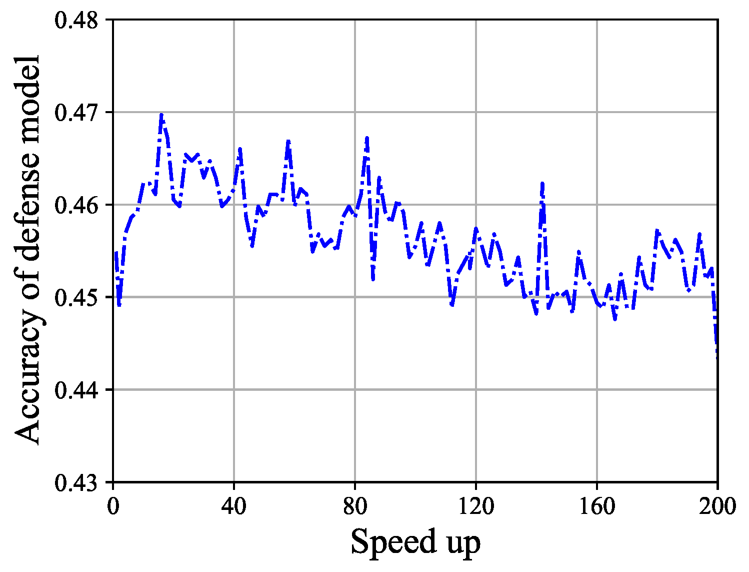
The accuracy of the defense model. The accuracy of the defense model before pruning is 0.4549. After pruning, the speed-up ranges from 2 to 200, with the maximum defense model accuracy being 0.4697 and the minimum defense model accuracy being 0.4433. It can be observed that the accuracy of the defense model does not change significantly. The result is shown in Figure 2. In Definition 1, when , the result satisfies the definition.
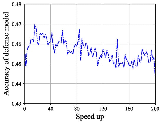
Figure 2.
The accuracy of the defense model varies with speed-up. It can be roughly observed that the accuracy ranges from 0.44 to 0.47, with a variation range of [0, 0.03].
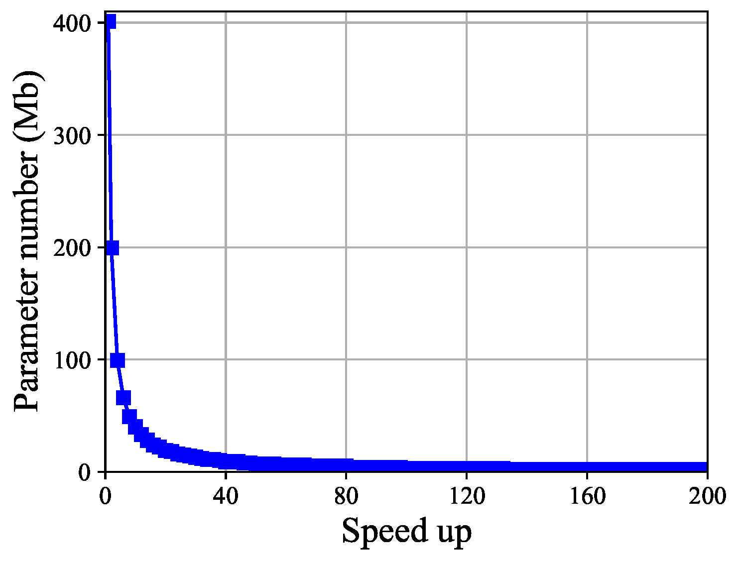
The number of parameters. The change in defense model parameter count with respect to speed-up is shown in Figure 3. The parameter count before model pruning is 401.04 Mb. After pruning, with speed-up ranging from 2 to 200, the minimum parameter count is 0.99 Mb, indicating a continuous decrease in parameter count. The minimum parameter count is achieved at a speed-up of 200. When , the result satisfies Definition 2. In addition to defending model parameters, another metric is floating point operations (FLOPs). Since the defense model adopts a fully connected network, the amount of defense model parameters and FLOPs are equivalent, so we will not display it separately.
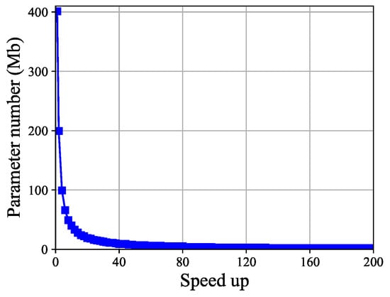
Figure 3.
The change in the number of defense model parameters with respect to speed-up. The parameter count gradually decreases as the speed-up increases, approaching zero around a speed-up of 80.
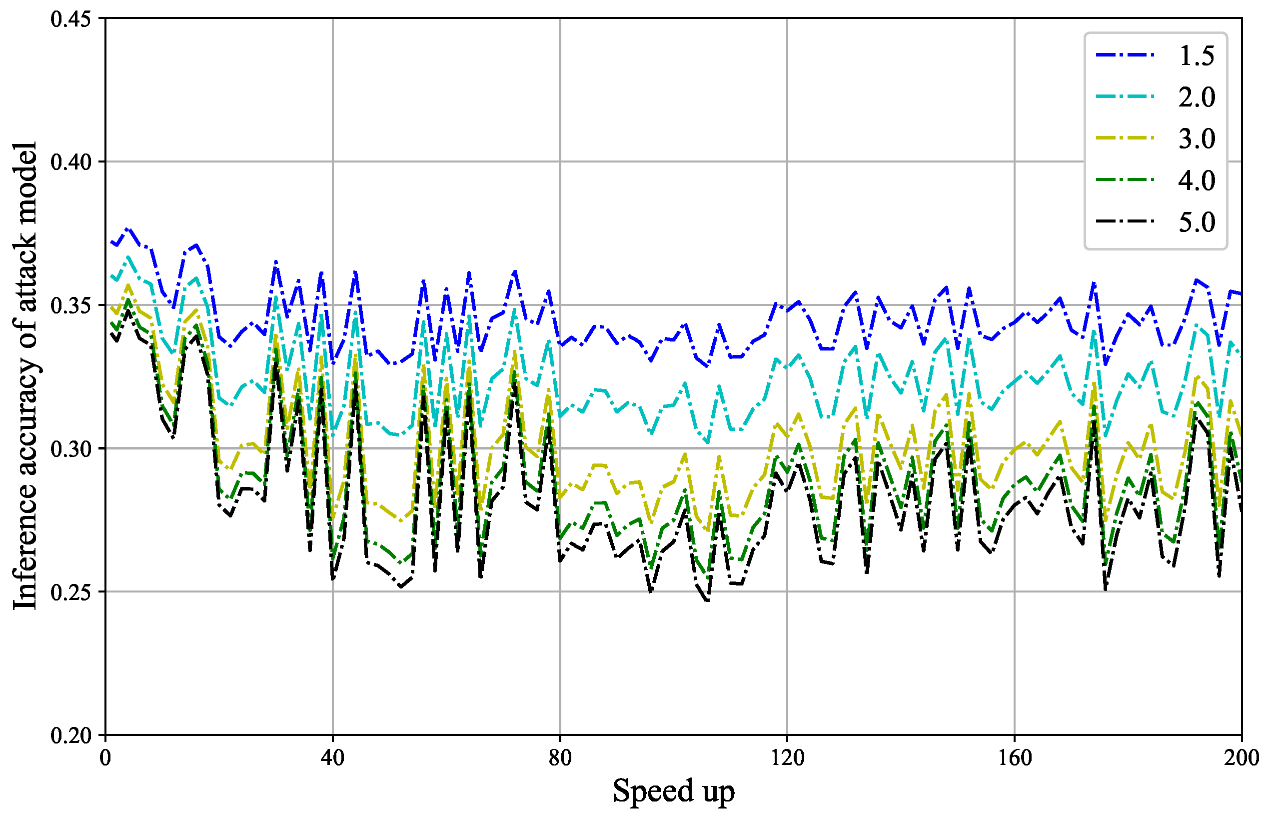
The inference accuracy of the attack model. The change in inference accuracy of the attack model with respect to speed-up under different noise budgets is shown in Figure 4. Prior to defense model pruning, the attack model’s inference accuracy at noise budgets of 1.5, 2.0, 3.0, 4.0, and 5.0 is 0.3721, 0.3603, 0.3492, 0.3439, and 0.3401, respectively.
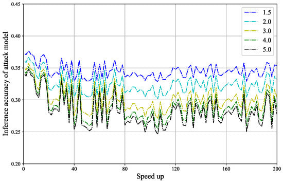
Figure 4.
The change in inference accuracy of the attack model with respect to speed-up under different noise budgets is shown. As the noise budget increases, the defense performance improves. At the same noise budget, the inference accuracy of the attack model is not very stable, but some points can be found where the inference accuracy is lower than before pruning.
- When the noise budget is set to 1.5, the maximum inference accuracy is 0.3771, and the minimum inference accuracy is 0.3283. When n = 0.0437, the results satisfy Definition 3.
- When the noise budget is set to 2.0, the maximum inference accuracy is 0.3666, and the minimum inference accuracy is 0.3020. When n = 0.0583, the results satisfy Definition 3.
- When the noise budget is set to 3.0, the maximum inference accuracy is 0.3569, and the minimum inference accuracy is 0.2707. When n = 0.0785, the results satisfy Definition 3.
- When the noise budget is set to 4.0, the maximum inference accuracy is 0.3518, and the minimum inference accuracy is 0.2548. When n = 0.0890, the results satisfy Definition 3.
- When the noise budget is set to 5.0, the maximum inference accuracy is 0.3480, and the minimum inference accuracy is 0.2459. When n = 0.0942, the results satisfy Definition 3.
At a speed-up of 80, the attack model’s inference accuracy corresponding to noise budgets of 1.5, 2.0, 3.0, 4.0, and 5.0 are 0.3354, 0.3111, 0.2827, 0.2686, and 0.2607, respectively. All of these values are lower than the inference accuracy prior to defense model pruning, indicating that the defense performance is better than before pruning. It can be observed that the relationship between model pruning and defense performance is not strictly monotonic, and in some cases, model pruning may improve defense effectiveness. This also demonstrates the feasibility of adding noise to the pruned models locally. However, this study is only an attempt, and researchers can explore other related areas for further investigation.
5.2.2. The Second SP-ASPP
We evaluate the second SP-ASPP from three aspects: defense model accuracy, model size, and attack inference accuracy, corresponding to Definitions 1–3 in the previous section, respectively.
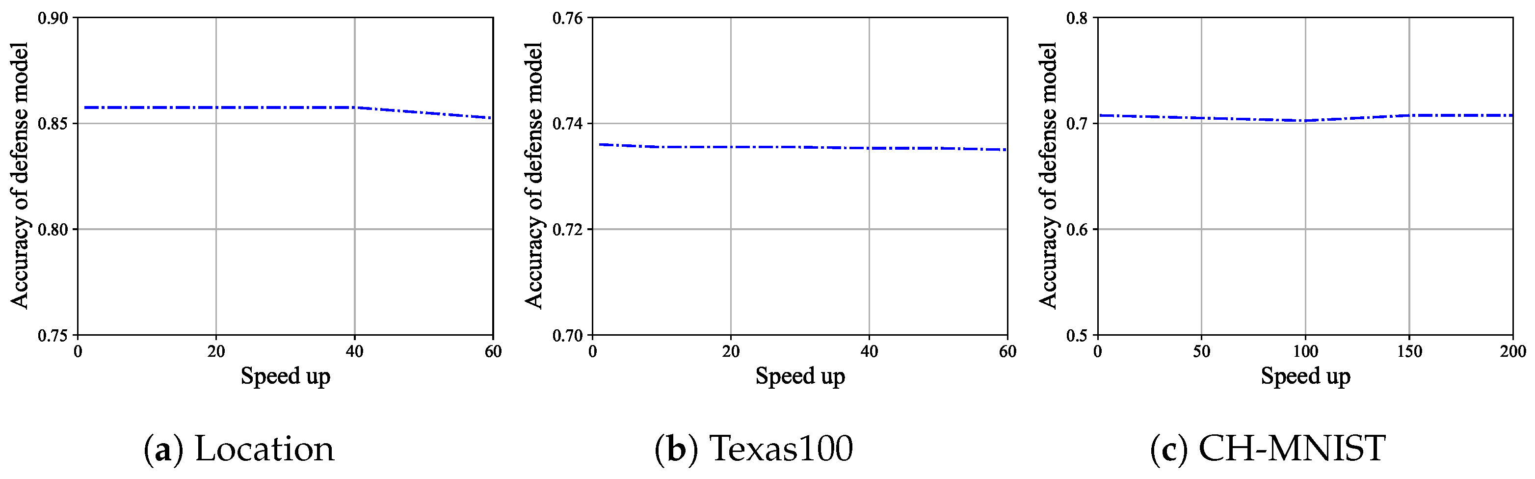
The accuracy of the defense model. For Location, the accuracy of the defense model before pruning is 0.8575. When speed up is set to 20, 40, and 60, the maximum accuracy of the defense model is 0.8575, and the minimum accuracy is 0.8525. It can be observed that the accuracy of the defense model does not vary much. This result is shown in Figure 5a. In Definition 1, when , the result satisfies this definition. For Texas100, the accuracy of the defense model before pruning is 0.736. When speed up is set to 20, 40, and 60, the maximum accuracy of the defense model is 0.7355, and the minimum accuracy is 0.7353. It can be observed that the accuracy of the defense model does not vary much. This result is shown in Figure 5b. In Definition 1, when , the result satisfies this definition. For CH-MNIST, the accuracy of the defense model before pruning is 0.7075. When speed up is set to 50, 100, 150, and 200, the maximum accuracy of the defense model is 0.7075, and the minimum accuracy is 0.7025. It can be observed that the accuracy of the defense model does not vary much. This result is shown in Figure 5c. In Definition 1, when , the result satisfies this definition.
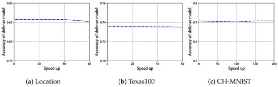
Figure 5.
The variationof the defense model’s accuracy with speed up for Location, Texas100, and CH-MNIST.
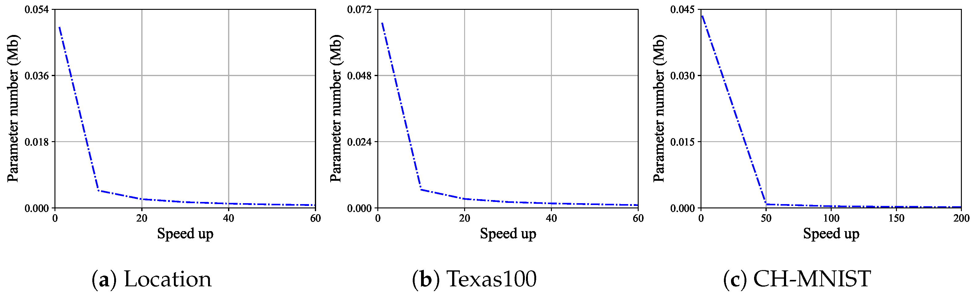
The number of parameters. The variation in the parameter size of the defense model with speed up is shown in Figure 6. For Location, the parameter size of the model before compression is 0.0492 Mb. When speed up is set to 20, 40, and 60, the minimum parameter size is 0.0008 Mb, which continuously decreases. The minimum parameter size is reached when the speed up is 60. When in Definition 2, the result satisfies this definition. For Texas100, before compression, the parameter size of the model is 0.0671 Mb. When speed up is set to 20, 40, and 60, the minimum parameter size is 0.0010 Mb, which continuously decreases. The minimum parameter size is reached when the speed up is 60. When in Definition 2, the result satisfies this definition. For CH-MNIST, before compression, the parameter size of the model is 0.0435 Mb. When speed up is set to 50, 100, 150, and 200, the minimum parameter size is 0.0002 Mb, which continuously decreases. The minimum parameter size is reached when the speed up is 200. When in Definition 2, the result satisfies this definition. It is expected that increasing the speed up will further reduce the model parameters. In addition to the parameter size of the defense model, another indicator is FLOPs. Since the defense model uses a fully connected network, the parameter size and FLOPs of the defense model are equal, so they are not shown separately.
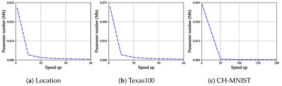
Figure 6.
For Location, Texas100, and CH-MNIS, the parameter number of the defense model varies with the change in speed up.
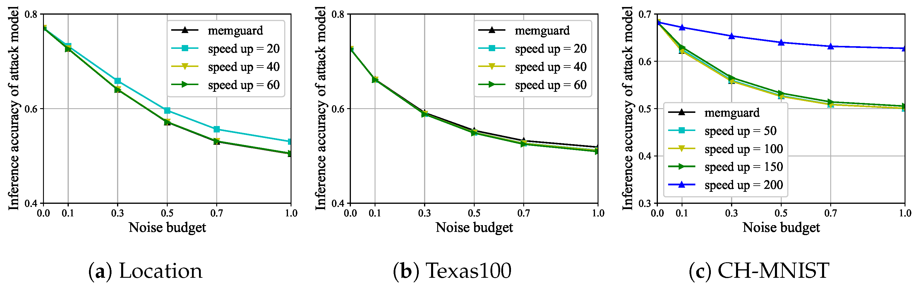
The inference accuracy of the attack model. The inference accuracy results of the attack model are shown in Figure 7. For the three datasets, Location, Texas100, and CH-MNIST, the defense effect of the defense model has remained essentially unchanged before and after pruning. For Location, the defense effect of the defense model slightly deteriorates at speed-up = 20, and other values can be selected for speed up during pruning. For the CH-MNIST, the defense effect of the defense model deteriorates at speed up = 200, and other values can also be selected for speed up during pruning. Obviously, the inference accuracy of the attack model satisfies Definition 3. We found that the upper limit of compression by speed up is related to the model’s own parameter size and the input and output dimensions of the model. The larger the model’s parameter size and the smaller the input and output dimensions of the model, the greater the potential for model pruning. Therefore, in practical applications, it is necessary to develop an appropriate speed up based on the actual situation, which can satisfy local adversarial sample privacy protection while not reducing the defense effect. So far, we have also demonstrated the feasibility of the second structural pruning-based adversarial sample privacy protection.
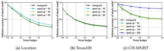
Figure 7.
For Location, Texas100, and CH-MNIST, the inference accuracy of the attack model varies with the noise budget and speed up.
In order to present the effectiveness of our approach more clearly, we showcase the results in the table below. In Table 1, we compare our first SP-ASPP with [2] and our second SP-ASPP with [3]. We will conduct separate comparisons for the four datasets and different speed-up ratios. In the ‘Methods’ column of Table 1, the value in parentheses represents the magnitude of speed-up. The inference accuracy of the attack model varies under different noise budgets. Therefore, we take the average of the attack model’s inference accuracy under different noise budgets to determine the final inference accuracy of the attack model. For Att, the considered noise magnitude budgets include 1.5, 2.0, 3.0, 4.0, and 5.0. For other datasets, the considered noise magnitude budgets are 0.1, 0.3, 0.5, 0.7, and 1.0.

Table 1.
The table displays the defense model accuracy, model parameter size, and inference accuracy of the attack models for different methods. In the ‘Methods’ column, the value in parentheses represents the magnitude of speed-up. The same attack model is applied to the same dataset. The inference accuracy of the attack model is the average value of inference accuracy under different noise magnitude budgets.
It can be observed that as the model pruning parameter speed up increases, the accuracy of the defense model remains relatively stable, the model parameter size decreases significantly, and there is a slight increase in the inference accuracy of the attack model. The change in defense model accuracy and the change in attack model inference accuracy are both minimal, indicating that the defense model’s effectiveness is relatively stable. This represents the SP-ASPPs proposed in this paper, which indeed significantly reduce model parameters while ensuring a certain level of defense effectiveness, demonstrating the effectiveness of the approach presented in this paper.
Through the above experiments, we found that using model pruning in adversarial sample privacy protections can significantly reduce the number of model parameters while ensuring a certain level of defense effectiveness. These findings indicate that structural pruning-based adversarial sample privacy protections have a certain degree of feasibility.
6. Conclusions
Previous adversarial sample privacy protections have mostly been centralized or have not considered the issue of hardware device limitations when conducting privacy protection, especially on the user’s local device. This work attempts to reduce the requirements of adversarial sample privacy protections on devices, making the privacy protection more locally friendly. Advanced model structure pruning techniques are used to prune and train the defense model structure, which is then distributed to users. Users complete the privacy protection process on the pruned model to obtain the noisy data. Experiments on real datasets show that our SP-ASPPs are efficient. Through the solution of this article, the practical use of LASPP is promoted. In fact, the schemes in [2,3] are not secure because the defense schemes of adversarial samples [31,32,33] continue to be proposed, requiring more robust privacy protections. However, we are confident that robust models can still be pruned, and this is also a future direction for research.
Author Contributions
The model and methodology of this paper were proposed by G.X. and Q.P. The experiments were designed and conducted by G.X. and G.H.; H.H. was responsible for the graphical work of the paper. The writing of the paper was completed by G.X., G.H. and Q.P.; H.H. reviewed the paper. G.X. and G.H. made revisions to the paper. All authors have read and agreed to the published version of the manuscript.
Funding
This work is supported by the National Key Research and Development Program of China under Grant 2022YFB3-102700; the National Natural Science Foundation of China under Grants 62132013, 62102295, 62276198, and 61902292; and the Key Research and Development Programs of Shaanxi under Grant 2021ZDLGY06-03.
Data Availability Statement
Data are contained within the article.
Acknowledgments
Thanks to the development teams behind PyTorch and other toolkits for providing convenient experimental tools. Thanks to Featurize for offering a convenient and efficient cloud service, and thanks to the anonymous reviewers for their meticulous review.
Conflicts of Interest
The authors declare no conflicts of interest.
References
- Szegedy, C.; Zaremba, W.; Sutskever, I.; Bruna, J.; Erhan, D.; Goodfellow, I.; Fergus, R. Intriguing properties of neural networks. arXiv 2013, arXiv:1312.6199. [Google Scholar]
- Jia, J.; Gong, N.Z. {AttriGuard}: A practical defense against attribute inference attacks via adversarial machine learning. In Proceedings of the 27th USENIX Security Symposium (USENIX Security 18), Baltimore, MD, USA, 15–17 August 2018; pp. 513–529. [Google Scholar]
- Jia, J.; Salem, A.; Backes, M.; Zhang, Y.; Gong, N.Z. Memguard: Defending against black-box membership inference attacks via adversarial examples. In Proceedings of the 2019 ACM SIGSAC Conference on Computer and Communications Security, London, UK, 11–15 November 2019; pp. 259–274. [Google Scholar]
- Shao, R.; Shi, Z.; Yi, J.; Chen, P.Y.; Hsieh, C.J. Robust text captchas using adversarial examples. In Proceedings of the 2022 IEEE International Conference on Big Data (Big Data), IEEE, Osaka, Japan, 17–20 December 2022; pp. 1495–1504. [Google Scholar]
- Papernot, N.; McDaniel, P.; Jha, S.; Fredrikson, M.; Celik, Z.B.; Swami, A. The limitations of deep learning in adversarial settings. In Proceedings of the 2016 IEEE European Symposium on Security and Privacy (EuroS&P), IEEE, Saarbrücken, Germany, 21–24 March 2016; pp. 372–387. [Google Scholar]
- Shokri, R.; Stronati, M.; Song, C.; Shmatikov, V. Membership inference attacks against machine learning models. In Proceedings of the 2017 IEEE Symposium on Security and Privacy (SP), IEEE, San Jose, CA, USA, 22–24 May 2017; pp. 3–18. [Google Scholar]
- Madry, A.; Makelov, A.; Schmidt, L.; Tsipras, D.; Vladu, A. Towards deep learning models resistant to adversarial attacks. arXiv 2017, arXiv:1706.06083. [Google Scholar]
- Dwork, C. Differential privacy. In Proceedings of the International Colloquium on Automata, Languages, and Programming; Springer: Cham, Switzeland, 2006; pp. 1–12. [Google Scholar]
- Shokri, R.; Theodorakopoulos, G.; Troncoso, C.; Hubaux, J.P.; Le Boudec, J.Y. Protecting location privacy: Optimal strategy against localization attacks. In Proceedings of the 2012 ACM Conference on Computer and Communications Security, Raleigh, NC, USA, 16–18 October 2012; pp. 617–627. [Google Scholar]
- Salamatian, S.; Zhang, A.; du Pin Calmon, F.; Bhamidipati, S.; Fawaz, N.; Kveton, B.; Oliveira, P.; Taft, N. Managing your private and public data: Bringing down inference attacks against your privacy. IEEE J. Sel. Top. Signal Process. 2015, 9, 1240–1255. [Google Scholar] [CrossRef]
- Xie, G.; Pei, Q. Towards Attack to MemGuard with Nonlocal-Means Method. Secur. Commun. Netw. 2022, 2022, 6272737. [Google Scholar] [CrossRef]
- Wang, T.; Blocki, J.; Li, N.; Jha, S. Locally differentially private protocols for frequency estimation. In Proceedings of the 26th USENIX Security Symposium (USENIX Security 17), Vancouver, BC, Canada, 16–18 August 2017; pp. 729–745. [Google Scholar]
- Ding, X.; Ding, G.; Guo, Y.; Han, J. Centripetal sgd for pruning very deep convolutional networks with complicated structure. In Proceedings of the IEEE/CVF Conference on Computer Vision and Pattern Recognition, Long Beach, CA, USA, 15–20 June 2019; pp. 4943–4953. [Google Scholar]
- You, Z.; Yan, K.; Ye, J.; Ma, M.; Wang, P. Gate decorator: Global filter pruning method for accelerating deep convolutional neural networks. arXiv 2019. [Google Scholar] [CrossRef]
- Fang, G.; Ma, X.; Song, M.; Mi, M.B.; Wang, X. Depgraph: Towards any structural pruning. In Proceedings of the IEEE/CVF Conference on Computer Vision and Pattern Recognition, Vancouver, BC, Canada, 17–24 June 2023; pp. 16091–16101. [Google Scholar]
- Shen, M.; Molchanov, P.; Yin, H.; Alvarez, J.M. When to prune? A policy towards early structural pruning. In Proceedings of the IEEE/CVF Conference on Computer Vision and Pattern Recognition, New Orleans, LA, USA, 18–24 June 2022; pp. 12247–12256. [Google Scholar]
- Gao, S.; Zhang, Z.; Zhang, Y.; Huang, F.; Huang, H. Structural Alignment for Network Pruning through Partial Regularization. In Proceedings of the IEEE/CVF International Conference on Computer Vision, Paris, France, 2–3 October 2023; pp. 17402–17412. [Google Scholar]
- Shen, M.; Yin, H.; Molchanov, P.; Mao, L.; Liu, J.; Alvarez, J.M. Structural pruning via latency-saliency knapsack. Adv. Neural Inf. Process. Syst. 2022, 35, 12894–12908. [Google Scholar]
- Fang, G.; Ma, X.; Wang, X. Structural Pruning for Diffusion Models. arXiv 2023, arXiv:2305.10924. [Google Scholar]
- Hou, Y.; Ma, Z.; Liu, C.; Wang, Z.; Loy, C.C. Network pruning via resource reallocation. Pattern Recognit. 2024, 145, 109886. [Google Scholar] [CrossRef]
- Ma, X.; Fang, G.; Wang, X. LLM-Pruner: On the Structural Pruning of Large Language Models. arXiv 2023, arXiv:2305.11627. [Google Scholar]
- Dong, X.; Chen, S.; Pan, S. Learning to prune deep neural networks via layer-wise optimal brain surgeon. arXiv 2017. [Google Scholar] [CrossRef]
- Guo, Y.; Yao, A.; Chen, Y. Dynamic network surgery for efficient dnns. arXiv 2016. [Google Scholar] [CrossRef]
- Park, S.; Lee, J.; Mo, S.; Shin, J. Lookahead: A far-sighted alternative of magnitude-based pruning. arXiv 2020, arXiv:2002.04809. [Google Scholar]
- Luo, J.H.; Wu, J. Neural network pruning with residual-connections and limited-data. In Proceedings of the IEEE/CVF Conference on Computer Vision and Pattern Recognition, Seattle, WA, USA, 13–19 June 2020; pp. 1458–1467. [Google Scholar]
- Yao, L.; Pi, R.; Xu, H.; Zhang, W.; Li, Z.; Zhang, T. Joint-detnas: Upgrade your detector with nas, pruning and dynamic distillation. In Proceedings of the IEEE/CVF Conference on Computer Vision and Pattern Recognition, Nashville, TN, USA, 20–25 June 2021; pp. 10175–10184. [Google Scholar]
- Li, T.; Lin, L. Anonymousnet: Natural face de-identification with measurable privacy. In Proceedings of the IEEE/CVF Conference on Computer Vision and Pattern Recognition Workshops, Long Beach, CA, USA, 16–17 June 2019. [Google Scholar]
- Salman, H.; Khaddaj, A.; Leclerc, G.; Ilyas, A.; Madry, A. Raising the cost of malicious ai-powered image editing. arXiv 2023, arXiv:2302.06588. [Google Scholar]
- Shan, S.; Cryan, J.; Wenger, E.; Zheng, H.; Hanocka, R.; Zhao, B.Y. Glaze: Protecting artists from style mimicry by text-to-image models. arXiv 2023, arXiv:2302.04222. [Google Scholar]
- Kullback, S.; Leibler, R.A. On information and sufficiency. Ann. Math. Stat. 1951, 22, 79–86. [Google Scholar] [CrossRef]
- Ma, X.; Li, B.; Wang, Y.; Erfani, S.M.; Wijewickrema, S.; Schoenebeck, G.; Song, D.; Houle, M.E.; Bailey, J. Characterizing adversarial subspaces using local intrinsic dimensionality. arXiv 2018, arXiv:1801.02613. [Google Scholar]
- Liu, Y.; Qin, Z.; Anwar, S.; Ji, P.; Kim, D.; Caldwell, S.; Gedeon, T. Invertible denoising network: A light solution for real noise removal. In Proceedings of the IEEE/CVF Conference on Computer Vision and Pattern Recognition, Nashville, TN, USA, 20–25 June 2021; pp. 13365–13374. [Google Scholar]
- Meng, D.; Chen, H. Magnet: A two-pronged defense against adversarial examples. In Proceedings of the 2017 ACM SIGSAC Conference on Computer and Communications Security, Dallas, TX, USA, 30 October–3 November 2017; pp. 135–147. [Google Scholar]
Disclaimer/Publisher’s Note: The statements, opinions and data contained in all publications are solely those of the individual author(s) and contributor(s) and not of MDPI and/or the editor(s). MDPI and/or the editor(s) disclaim responsibility for any injury to people or property resulting from any ideas, methods, instructions or products referred to in the content. |
© 2024 by the authors. Licensee MDPI, Basel, Switzerland. This article is an open access article distributed under the terms and conditions of the Creative Commons Attribution (CC BY) license (https://creativecommons.org/licenses/by/4.0/).