An MTBWO Algorithm Based on BiGRU Model

Abstract

To address the challenge of distinguishing the health status of bearings, in this paper, a health index (HI) is developed through utilization of the multiple target time-varying black widow optimization–bidirectional gating recurrent unit (MTBWO-BiGRU) model and the Bray–Curtis distance. This index offers a visual representation of the health status of bearings, enabling more intuitive monitoring and prediction. The first step involves utilizing L1 regularization to extract effective features as degradation elements from the current bearing vibration data. Additionally, the characteristics of the initial time window of the vibration data serve as the health features. Next, the HI of the bearing is constructed by computing the Bray–Curtis distance between the bearing’s degradation characteristics and health features. The cloud monitoring platform constantly tracks the health of the bearing and employs the MTBWO-BiGRU model to anticipate the forthcoming state of health. The platform generates an immediate alert when the HI of the bearing overtakes the alteration rate threshold and foresees the condition of the bearing. We compare the MTBWO-BiGRU model with the bidirectional long short-term memory (BiLSTM) and BiGRU models. The results indicate an accuracy level of 92.57%, which is evidently higher than that obtained when using the other two models. Moreover, the MTBWO-BiGRU model is lighter, demonstrating the practicality of the proposed approach.

1. Introduction

In the industrial sector, bearings play a crucial role in various mechanical equipment. However, as the equipment operation time is extended and working conditions change, monitoring and maintaining the health status of bearings become increasingly challenging. Bearing failures not only result in equipment downtime and production losses but can also lead to serious safety incidents, imposing significant economic burdens and reputation risks on enterprises. Consequently, achieving effective monitoring, early fault diagnosis and precise maintenance of bearings has emerged as a pivotal challenge in today’s industry.

In theory, the health index is an important component in the field of health management and is designed to predict the level of damage caused by failures based on current and future operating conditions and working environments, thereby predicting the point at which a piece of machinery or equipment will fail to perform its function within the expected lifetime of the machinery or equipment. Based on existing research, there are three broad categories of approaches: data-driven approaches, mathematical model-based approaches and a fusion of the two. Data-driven prediction methods are mainly based on collecting a large amount of mechanical equipment operation data and using machine learning, deep mining and other technologies to discover trends and correlations in the data for prediction; mathematical model-based prediction methods are based on analyzing the failure mechanism of the equipment and predicting it by building a corresponding mathematical model; and methods based on the fusion of the two are based on combining mathematical model-based methods with data-driven methods.

Obtaining a large amount of bearing operating data is key to data-driven methods, but this can involve the installation of sensors and data collection. The quality and accuracy of the data are critical to the reliability of the prediction. Mathematical modeling methods require a deep understanding of bearing failure mechanisms. However, due to the complexity of the bearing operating environment, it can be difficult to establish accurate mathematical models. The variety and complexity of different types of bearings and their operating environments can be enormous, making it difficult to develop general prediction models. Effectively integrating data-driven and mathematical modeling methods is a complex task, which requires overcoming the differences between the two methods and finding the best integration strategy.

Overcoming these challenges and achieving predictive bearing health monitoring requires an innovative approach. We propose a two-way gated recurrent unit model integrated with L1 regularization and complemented by health indicators derived from the Bray–Curtis distance. These indicators are seamlessly integrated into a real-time monitoring platform to predict the future health status of bearings.

Initially, the method involves extracting time-domain characteristics from historical vibration signal sequences of the bearings. As the bearing continues to operate, damage accumulates, gradually reducing its health. In the on-line phase, current degradation characteristics are fed into the model to predict future degradation trends. The Bray–Curtis distance between the health features and the initial state of the bearing is then calculated to generate health indicators. The thresholds for abnormal changes in these indicators are set, triggering real-time alarms on the cloud platform when the rate of change exceeds pre-defined limits.

This proactive approach enables timely intervention, reducing the risk of significant economic losses due to machine damage. By preventing such losses, the proposed method not only enhances the reliability and longevity of industrial equipment but also safeguards the operational continuity and financial stability of companies.

2. Literature Review

S. Wan et al. [1] introduced an approach to bearing fault detection with their multi-sensor information coupling network (MICN), which processes signals from various sensors to extract in-depth features independently and fuse them layer by layer. The proposed model features a novel feature-level information coupling technique, which utilizes a mutual attention mechanism during the multi-layer feature fusion process. However, the introduction of multiple sensors and a mutual attention mechanism may increase the complexity of the model, both in terms of implementation and computational requirements.

Duan and colleagues [2] developed the adaptive EMUW method for improving MUDW. They utilized waveform trend (WT) to compensate for the shortcomings of MOs, thus eliminating the interference caused by random impulses. By assessing the similarity between WT signals of neighboring levels, they were able to determine the appropriate number of decomposition levels for EMUW. The final step involved reconstructing the signal using the sub-signals extracted from the decomposition. The adaptive nature and the incorporation of waveform trend compensation might add complexity to the implementation and understanding of the method.

Yang et al. [3] presented an approach for bearing status feature extraction utilizing variational mode decomposition (VMD) and improved envelope spectrum entropy (IESE). The vibrational signals of the bearing are initially decomposed into different intrinsic mode functions (IMFs) by VMD. Subsequently, the envelope spectrum entropy (ESE) of each IMF is calculated. The IESE is then obtained by reconstructing the ESE to form original feature sets. These original feature sets are fused using joint approximate diagonalization eigen (JADE) to create a new set. This new feature set is then employed to train and test a support vector machine (SVM) for bearing status identification. Despite the effectiveness of VMD in decomposing vibrational signals, there might be instances where it fails to capture all the relevant information, potentially leading to the loss of important features during decomposition.

Xue et al. [4] described a method using a multi-scale deep belief network (DBN) with an integrated attention mechanism to extract the fundamental properties of vibration signals at various scales. The process includes four primary stages: pre-processing of multi-scale data, feature extraction, feature fusion and fault classification. Technical term abbreviations were explained when first used in this research. The language was kept formal and objective to adhere to academic writing quality. Consistent citation and formatting features were maintained. The main advancements made are the multi-scale feature extraction, which employs a multi-scale DBN algorithm, and feature fusion using an attention mechanism. The University of Ottawa’s benchmark dataset was employed to assess the efficacy and benefits of the proposed technique. The inner workings of deep-learning models, especially complex architectures, such as multi-scale DBNs, can be challenging to interpret, making it difficult to understand how and why certain features are being extracted and fused.

X. Liu et al. [5] introduced a technique for the diagnosis of bearing faults that resist noise using an improved recurrence plot (RP) and a convolutional neural network (CNN). RP aids in the detection of non-linear signals in the bearing’s vibration, while the CNN self-learns the non-linear information extracted from the recurrent plot to accomplish the classification task. Convolutional neural networks (CNNs) are often considered black-box models, making it challenging to interpret how they arrive at classification decisions based on the features extracted from recurrence plots.

Z. Zhao et al. [6] combined stacked denoised autoencoder (SDAE) and self-organizing maps (SOM) to construct a one-dimensional HI curve based on the original vibration signal. This health index (HI) curve was then fed into the MS-LSTM network to predict the long-term future trend. Finally, the remaining useful life (RUL) was calculated based on a failure threshold. Given that SDAE, SOM and MS-LSTM networks are diverse models with varying architectures and learning styles, effectively integrating them and ensuring synergy between them can pose challenges.

K. Zou et al. [7] proposed a fault prediction model, which relies on an HI created by a feature fusion algorithm combined with a gated recurrent unit (GRU) network. They constructed a new HI incorporating root mean square, peak, root mean square frequency and frequency center of gravity for feature fusion. The GRU network served as the core for building the prediction model of health indicators. Q. Ni et al. [8] introduced a scheme for inferring degradation progression by developing a novel HI. Subsequently, they employed a gated recurrent unit network to predict the RUL of the bearing system. Additionally, they integrated the Bayesian optimization algorithm to adaptively tune the optimal hyperparameters. However, it is worth noting that since GRU can only consider information up to the current time step, it might struggle when modeling bidirectional contexts.

H. Wang et al. [9] introduced a method for predicting the remaining useful life (RUL) of bearings based on the multiple-feature fusion health indicator (MFF-HI) and weighted temporal convolution network (WTCN). The MFF-HI is created through an MFF depth network (MFFDN) employing the MISH activation function to extract and fuse degradation information from bearing time-domain features. While their proposed approach shows promise, its complexity and potential challenges related to interpretability, activation functions and network architecture should be thoroughly assessed and validated across various real-world scenarios before considering widespread adoption.

C. Yang et al. [10] proposed a technique for decomposing the vibration signal of rolling bearings into intrinsic scale components using PCHIP-LCD. They select effective components based on K-C criteria, extract a multi-dimensional degradation feature set and calculate the sensitive degradation indicator IICAMD by fusing IICA and MD. False fluctuations in IICAMD are corrected using GM to derive the health indicator (HI). Subsequently, the start prediction time based on HI is determined, and a GRNN model based on HI is employed to predict the RUL of the rolling bearing. The effectiveness of this approach could rely heavily on the selection of parameters and thresholds, such as those involved in decomposition.

M. He and W. Guo [11] proposed an improved clustering algorithm called the Hellinger distance-based regularized Gaussian mixture model (HRGMM). In this model, the Hellinger distance is incorporated to measure the similarity between probability distributions (PDs) of raw data. The manifold regularized GMM is then enhanced to differentiate bearing performance changes. Second, we construct a new health indicator (HI) combining the Jensen–Renyi divergence and improved confidence value to normalize the difference in PDs between the test condition and healthy condition.

The above research works present the following problems despite the good results: (1) They are prone to issues such as gradient explosion and vanishing gradients; (2) Extracting vibration signal features in environments with strong noise proves challenging; (3) The network structures are complex, making learning difficult and limiting generalization; (4) Certain methods rely heavily on precise parameter and threshold selection in decomposition, necessitating extensive experimentation and optimization efforts.

3. Materials and Methods

3.1. System Overview

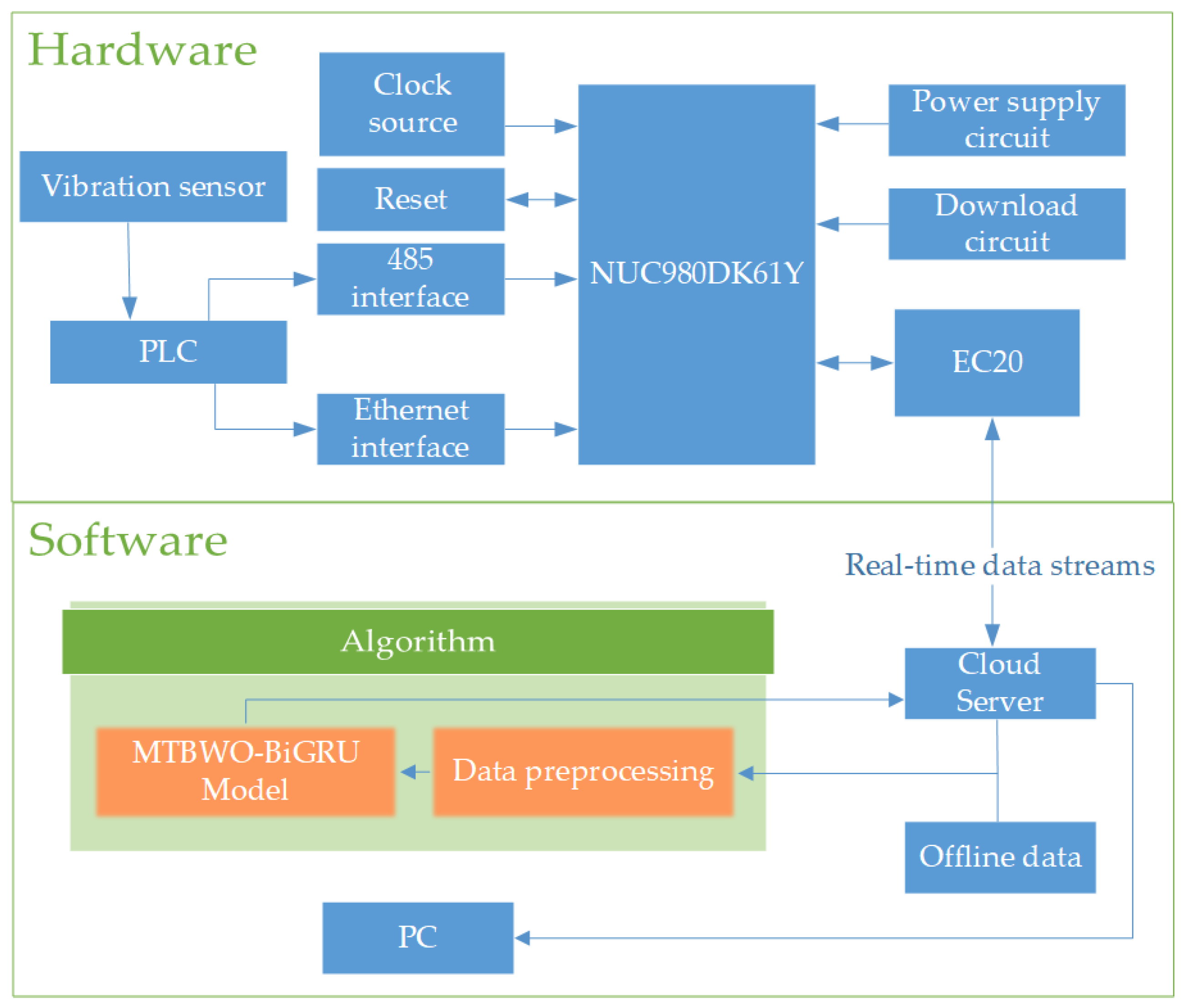
The present article details the architecture of a machine health monitoring system using NUC980 technology. The system incorporates industrial vibration sensors, a programmable logic controller (PLC), an NUC980DK61Y microprocessor, an EC20 communication module, an MQTT server and a monitoring terminal. Technical abbreviations will be explained upon first use.

NUC980 is an embedded microcontroller, which is widely used in embedded systems, including industrial control, automotive electronics, home appliances, smart home and other fields, with powerful processing capabilities and rich peripheral interfaces to meet the needs of different applications. It adopts an advanced low-power design, which enables low power consumption while maintaining high performance. This makes them ideal for battery-powered applications, which require extended operation. The NUC980DK61Y microprocessor serves as the core of the system’s hardware section, collecting data from the PLC through the Ethernet and 485 interfaces.

The EC20 embedded communication module facilitates data transmission between the NUC980 and the MQTT server [12] using the PCI-E interface, with it serving as an LTE module. Data are then transmitted to a cloud server via the MQTT protocol where they are stored, and a cloud monitoring platform is established to monitor bearing health status information.

The EC20 module is an embedded communication module, which is typically used to provide wireless connectivity capabilities, such as 4G LTE, 3G and 2G.

(1)

The EC20 module supports a variety of communication technologies, including LTE, WCDMA, TD-SCDMA, GSM and the global navigation satellite system (GNSS), which makes it possible to communicate in different network environments.

(2)

The EC20 module has high-speed data transmission capability, enabling reliable data communication. This makes it suitable for various applications, such as the internet of things (IoT), remote monitoring and telematics.

(3)

Low-power design: To meet the needs of mobile devices and portable applications, EC20 modules are often designed with low power consumption to extend the battery life of devices and reduce energy consumption.

MQTT is a lightweight messaging protocol designed for use in situations where a small code footprint is required and network bandwidth is limited or unreliable. In the context of communication systems, MQTT plays a crucial role in facilitating efficient, reliable and real-time communication between devices or clients in a publish/subscribe messaging model.

The hardware system includes vibration sensors, a PLC, a data acquisition module, a cloud server and a PC. The present paper presents the design of the data acquisition module, comprising a data acquisition end and a microprocessor control end. Please refer to Figure 1 for the system framework diagram.

The data acquisition end consists of multiple vibration sensors connected to the PLC, which stores the sensor data. The microprocessor control end is composed of the NUC980 chip, a reset circuit, a download circuit, a power supply circuit, a clock source and a wireless communication circuit. The wireless communication circuit is composed of EC20 modules. Paired with the MQTT library, it facilitates data transmission and exchange with the server.

3.2. L1 Regularization Introduction

To extract the informative features from the vibration signals, we employed the L1 regularization model [13]. This model includes an L1 norm penalty term in the loss function, enabling us to minimize the sum of the target function and the L1 norm of the features, leading to feature selection. First, we must prepare the features and corresponding target variables based on the specific conditions of the dataset and task. Next, a linear model with L1 regularization, such as the Lasso regression model, is utilized to fit the training data. These models integrate an L1 regularization term in the loss function.

While training the model, L1 regularization adapts the weights of the features, resulting in some of the feature weights becoming zero. This occurs because L1 regularization encourages sparsity in the feature weights by minimizing the sum of the target function and the L1 norm of the features. Based on the feature weights in the model, non-zero weight features can be selected, indicating their significant impact on the target variable, i.e., the desired features.

Therefore, the L1 regularization model is implemented to extract vibration signal features with high information content. To summarize, this feature extraction method is effective in identifying important features. By incorporating the L1 regularization term into the loss function, the model modifies the feature weights, encouraging sparsity and recognizing features, which hold a substantial impact on the target variable.

3.3. BiGRU Model

BiGRU is a model architecture based on recurrent neural networks (RNNs) used for modeling and learning from time series data. It combines bidirectionality and gating mechanisms to better capture long-term dependencies in sequential data.

The BiGRU model [14] used in this paper reduces parameters by combining the hidden state with the cell state and incorporates two unique gates: the reset gate and the update gate. A unidirectional GRU model can only access information from the forward time steps. However, in tasks such as predicting the health status of bearings, the model needs to learn contextual information and extract deep features from the input. The BiGRU model consists of two opposite-directional unidirectional GRUs: the forward GRU captures information from previous time steps, while the backward GRU captures information from future time steps. The outputs of the two GRUs with opposite directions jointly determine the output at the current position. The update gate output, denoted as ‘z’, is calculated using the following Equation (1).

$$\mathrm{z}\left(\mathrm{t}\right)=\sigma \left({\mathrm{V}}_{\mathrm{z}}\mathrm{X}\left(\mathrm{t}\right){+\mathrm{W}}_{\mathrm{z}}\mathrm{h}\left(\mathrm{t}-1\right)\right)$$

(1)

In the given context, the current input unit is represented by $X\left(t\right)$, while the weights are represented by $V_z$ and $W_z$; $h\left(t-1\right)$ refers to the stored data of the previous unit, which can store feature information. The activation function, which has a range of 0–1, is represented by $\sigma$. By utilizing these parameters, the network is able to access past data. The reset gate is calculated using the following Equation (2).

$$\mathrm{r}\left(\mathrm{t}\right)=\sigma \left({\mathrm{V}}_{\mathrm{r}}\mathrm{X}\left(\mathrm{t}\right){+\mathrm{W}}_{\mathrm{r}}\mathrm{h}\left(\mathrm{t}-1\right)\right)$$

(2)

Similar to the update gate, the addition is passed through the activation function. The reset gate is responsible for storing pertinent information from the past when introducing new memory content, and it is calculated using Equation (3).

$$\mathrm{c}\left(\mathrm{t}\right)=\tan \mathrm{h}\left(\mathrm{VX}\left(\mathrm{t}\right)+\mathrm{r}\left(\mathrm{t}\right)\odot \mathrm{Wh}\left(\mathrm{t}-1\right)\right)$$

(3)

Here, $\tan \mathrm{h}$ represents the non-linear activation function. The reset gate r determines the information to be discarded, which is $Wh\left(t-1\right)$. Finally, $h\left(t\right)$ stores the information of the current unit and transfers it to the network, which is calculated using Equation (4).

$$\mathrm{h}\left(\mathrm{t}\right)=\mathrm{z}\left(\mathrm{t}\right)\odot \mathrm{h}\left(\mathrm{t}-1\right)+\left(1-\mathrm{z}\left(\mathrm{t}\right)\right)\odot \mathrm{h}\left(\mathrm{t}\right)$$

(4)

3.4. Algorithm Design

3.4.1. MTBWO Algorithm

The paper presents a MTBWO algorithm, a type of swarm intelligence optimization algorithm. The algorithm is an extension of the BWOA [15], which includes multi-objective optimization and time-varying iteration arrays. This modification boosts the algorithm’s capacity for global search and convergence improvement.

In the context of this algorithm, the spiders display two distinct mating behaviors on a spider’s web. Each spider represents a candidate solution for an optimization problem, and its ability to survive aligns with the fitness function. The spider with the strongest survival capability determines the optimal solution. The n individual spider vectors are represented as a one-dimensional array [$A_1,A_2,\dots ,A_n$] [16]. Every time, two parents are randomly chosen for reproduction. The variable is introduced, initially assigned a random value between 0 and 1, and adaptively decreased based on the number of iterations. Both parents reproduce according to the cross-over rate.

3.4.2. Data Pre-Processing Algorithm Design

As the sensor generates a large amount of vibration data in real time, in order to extract the feature information in the shortest processing time, this study first slices the vibration data into equal-length sequences and then samples the vibration sequences at equal intervals to form a number of one-dimensional array sequences. In order to characterize the time-domain features of the vibration data, we selected the nine formulae in

Table 1. Equations for calculating the time-domain features of the vibration signals.

Variable Name	Time-Domain Feature	Equation
$F_1$	Maximum absolute value	${\mathrm{MAX}}_{\mathrm{i}}=\left|\max \left({\mathrm{x}}_{\mathrm{i}}\right)\right|$
$F_2$	Root mean square	${\mathrm{RMS}}_{\mathrm{i}}=\sqrt{\frac{1}{\mathrm{N}}{\displaystyle \sum _{\mathrm{i}=1}^{\mathrm{N}}{\left({\mathrm{x}}_{\mathrm{i}}- \overline{\mathrm{x}}\right)}^2}}$
$F_3$	Peak-to-peak	$\mathrm{p}{.\mathrm{p}}_{\mathrm{i}}=\max \left({\mathrm{x}}_{\mathrm{i}}\right)-\min \left({\mathrm{x}}_{\mathrm{i}}\right)$
$F_4$	Skewness	${\mathrm{skewness}}_{\mathrm{i}}=\frac{1}{\mathrm{N}}{\displaystyle \sum _{\mathrm{n}=1}^{\mathrm{N}}{\left(\frac{{(\mathrm{x}}_{\mathrm{i}}- \overline{\mathrm{x}})}{\mathrm{std}\left(\mathrm{x}\right)}\right)}^3}$
$F_5$	Kurtosis	${\mathrm{Kurtosis}}_{\mathrm{i}}=\frac{1}{\mathrm{N}}{\displaystyle \sum _{\mathrm{n}=1}^{\mathrm{N}}{\left[{\mathrm{x}}_{\mathrm{i}}- \overline{\mathrm{x}}\right]}^4}$
$F_6$	Minimum value	${\mathrm{Min}}_{\mathrm{i}}=\min \left({\mathrm{x}}_{\mathrm{i}}\right)$
$F_7$	Root square amplitude	${\mathrm{RA}}_{\mathrm{i}}=\frac{1}{\mathrm{N}}{\left({\displaystyle \sum _{\mathrm{n}=1}^{\mathrm{N}}\sqrt{\left|{\mathrm{x}}_{\mathrm{i}}\right|}}\right)}^2$
$F_8$	Variance	${\mathrm{Var}}_{\mathrm{i}}=\frac{1}{\mathrm{N}-1}{\displaystyle \sum _{\mathrm{i}=1}^{\mathrm{N}}{\left({\mathrm{x}}_{\mathrm{i}}- \overline{\mathrm{x}}\right)}^2}$
$F_9$	Pulse factor	${\mathrm{X}}_{\mathrm{PulseF}\mathrm{i}}=\frac{\max \left(\left|{\mathrm{x}}_{\mathrm{i}}\right|\right)}{ \overline{\mathrm{x}}}$

. These formulae cover the root mean square, variance, peak-to-peak value and other key features of the vibration signals, which comprehensively and effectively describe the time-domain characteristics of the vibration data, so as to achieve efficient processing and feature extraction of the vibration data.

After extracting the time-domain features, they are normalized using Equation (5).

$$\mathrm{X}=\frac{\mathrm{x}-{\mathrm{x}}_{\min }}{{\mathrm{x}}_{\max }-{\mathrm{x}}_{\min }}$$

(5)

The resulting feature sequence serves as the input samples for the model, enabling the construction of a feature learning network. Algorithm 1 steps are as follows.

Algorithm 1 Data pre-processing algorithm

Input: Horizontal vibration signal with length 123 × 32,679. Output: ${\mathrm{F}}_1,{\mathrm{F}}_2,{\mathrm{F}}_3,{\mathrm{F}}_4,{\mathrm{F}}_5,{\mathrm{F}}_6,{\mathrm{F}}_7,{\mathrm{F}}_8,{\mathrm{F}}_9$ with size 123.

1: for I from 1 to 123, do 2:  for j from 1 to 32,679, do 3:    Calculate ${\mathrm{F}}_1,{\mathrm{F}}_2,{\mathrm{F}}_3,{\mathrm{F}}_4,{\mathrm{F}}_5,{\mathrm{F}}_6,{\mathrm{F}}_7,{\mathrm{F}}_8,{\mathrm{F}}_9$ via Table 1 4:  end for 5: end for 6: for i from 1 to 123, do 7:   $\mathrm{F}=\left(\mathrm{F}-{\mathrm{F}}_{\min }\right)/\left({\mathrm{F}}_{\max }-{\mathrm{F}}_{\min }\right)$ 8: end for

3.4.3. HI Construction Algorithm

Constructing a bearing health index becomes particularly critical as the data to be tested are generated in a real-time environment, with the data consisting of both historical data and data monitored in real time. The accuracy of this process has a direct impact on the accurate monitoring of the condition of the bearings, thus improving the reliability and life of the machine and equipment.

In this paper, we chose to use a combination of the BiGRU model and the Bray–Curtis distance to construct the health index of the bearings. The BiGRU model extracts the effective time-domain features from all the time-domain features obtained from Table 1 through L1 regularization, while the Bray–Curtis distance quantifies the relationship between degradation features and health features, thus visually expressing the bearing’s health status. Algorithm 2 steps are as follows.

Algorithm 2 HI Construction Algorithm

Input: ${\mathrm{F}}_1,{\mathrm{F}}_2,{\mathrm{F}}_3,{\mathrm{F}}_4,{\mathrm{F}}_5,{\mathrm{F}}_6,{\mathrm{F}}_7,{\mathrm{F}}_8,{\mathrm{F}}_9$ with size 123 Output: HI with size 118

Parameter Statements: Population: {$\mathrm{Layers},\mathrm{cells},\mathrm{learing}\mathrm{rate},\mathrm{steps}$}             Loss: MSE of the MTBWO-BiGRU model             F:${\mathrm{F}}_1,{\mathrm{F}}_2,{\mathrm{F}}_3,{\mathrm{F}}_4,{\mathrm{F}}_5,{\mathrm{F}}_6,{\mathrm{F}}_7,{\mathrm{F}}_8,{\mathrm{F}}_9$ 1: $\alpha ,\beta ϵ\left[0,1\right]$ 2: Define y to be a set of upward trending arrays 3: Calculate the correlation between F and y 4: Selection of F with positive correlation 5: Divide the first 70% F into the training set, 30% of F after division is the test set 6: Create the MTBWO-BiGRU model 7: Choose ${\mathrm{Population}}_{\mathrm{i},1}$ randomly 8: Calculate Loss_best 9: for n from 1 to 50, do 10:   ${\mathrm{Population}}_{\mathrm{i},1}=\alpha .{\ast \mathrm{Population}}_{\mathrm{i},1}+\left(1-\alpha \right).{\ast \mathrm{Population}}_{\mathrm{i},2}$ 11:   ${\mathrm{Population}}_{\mathrm{i},2}=\beta .{\ast \mathrm{Population}}_{\mathrm{i},2}+\left(1-\beta \right).{\ast \mathrm{Population}}_{\mathrm{i},1}$ 12:  Calculate Loss 13:  if Loss < Loss_best 14:    Loss_best=Loss 15: end for 16: print Population 17: input the training set 18: for epoch from 1 to 300, do 19:  Calculate Loss 20: end for 21: if Loss>0.1 continue Step 18–20 22: Output the predicted data ${\mathrm{F}}_{\mathrm{degenrative},\mathrm{i}}$ 23: ${\mathrm{F}}_{\mathrm{healthy},\mathrm{i}}$ = F in the first time window 24: $\mathrm{HI}=1-\raisebox{1ex}{${\displaystyle \sum _{\mathrm{i}=1}^{\mathrm{N}}}\left|{\mathrm{F}}_{\mathrm{healthy},\mathrm{i}}-{\mathrm{F}}_{\mathrm{degenrative},\mathrm{i}}\right|$}\!\left/ \!\raisebox{-1ex}{${\displaystyle \sum _{\mathrm{i}=1}^{\mathrm{N}}{\mathrm{F}}_{\mathrm{healthy},\mathrm{i}}+{\displaystyle \sum _{\mathrm{i}=1}^{\mathrm{N}}{\mathrm{F}}_{\mathrm{degenrative},\mathrm{i}}}}$}\right.$

4. Results

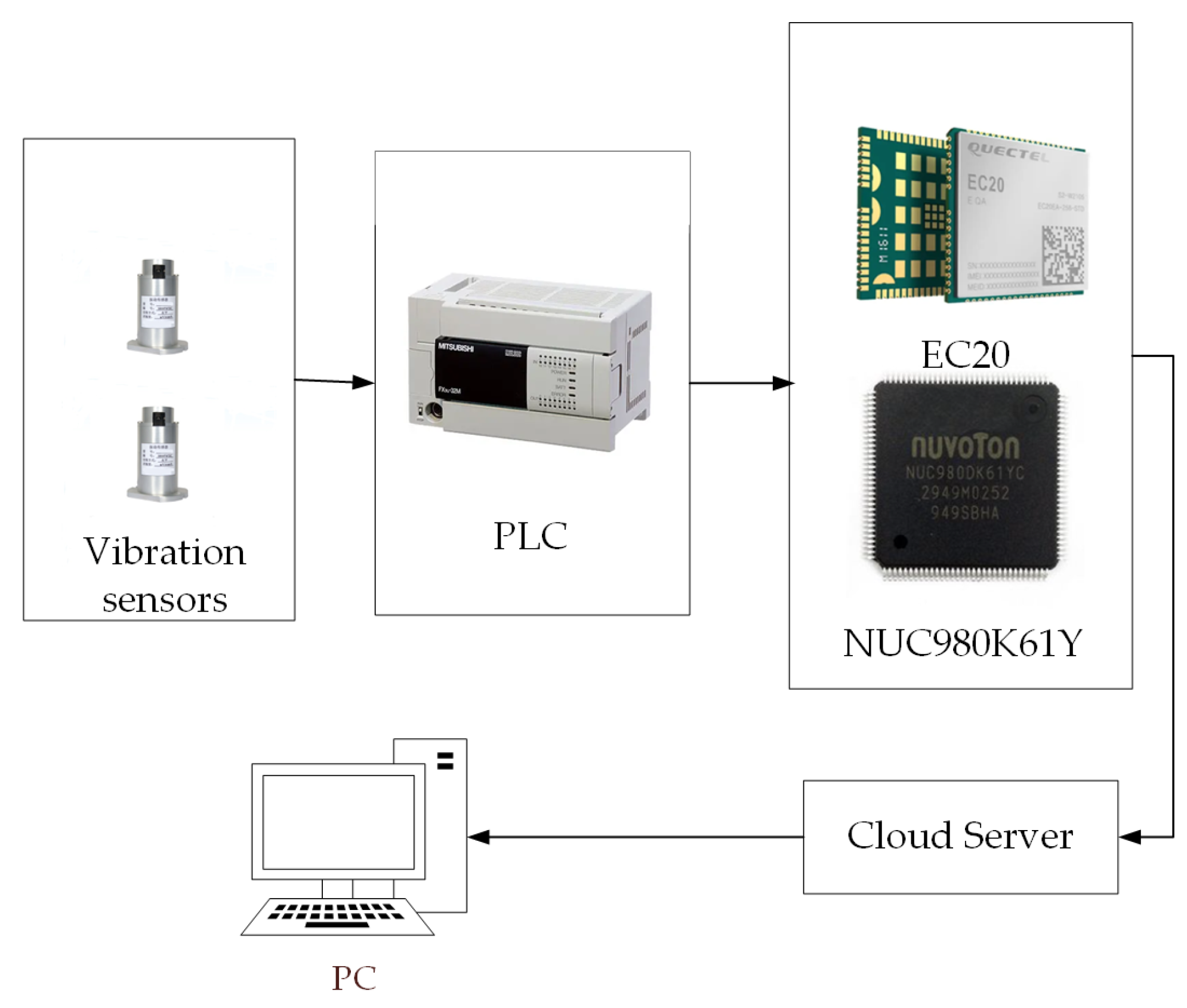
The computer system employs an AMD Ryzen 7 central processor with eight cores operating at 3.2 GHz and is compatible with the Windows 10 operating system. The embedded platform utilizes the RT-thread real-time operating system. Fundamental network server functionalities are implemented using Python modules, such as socket and http.server. The training model is implemented in Python using the PyTorch library, and HTML web development is carried out through the utilization of JavaScript. The overall architecture of the system is shown in Figure 2. The vibration sensors’ model is VVB001. The sensors’ frequency range is 2–10,000 hz. The PLC model is Mitsubishi FX5U.

4.1. Training of the Model

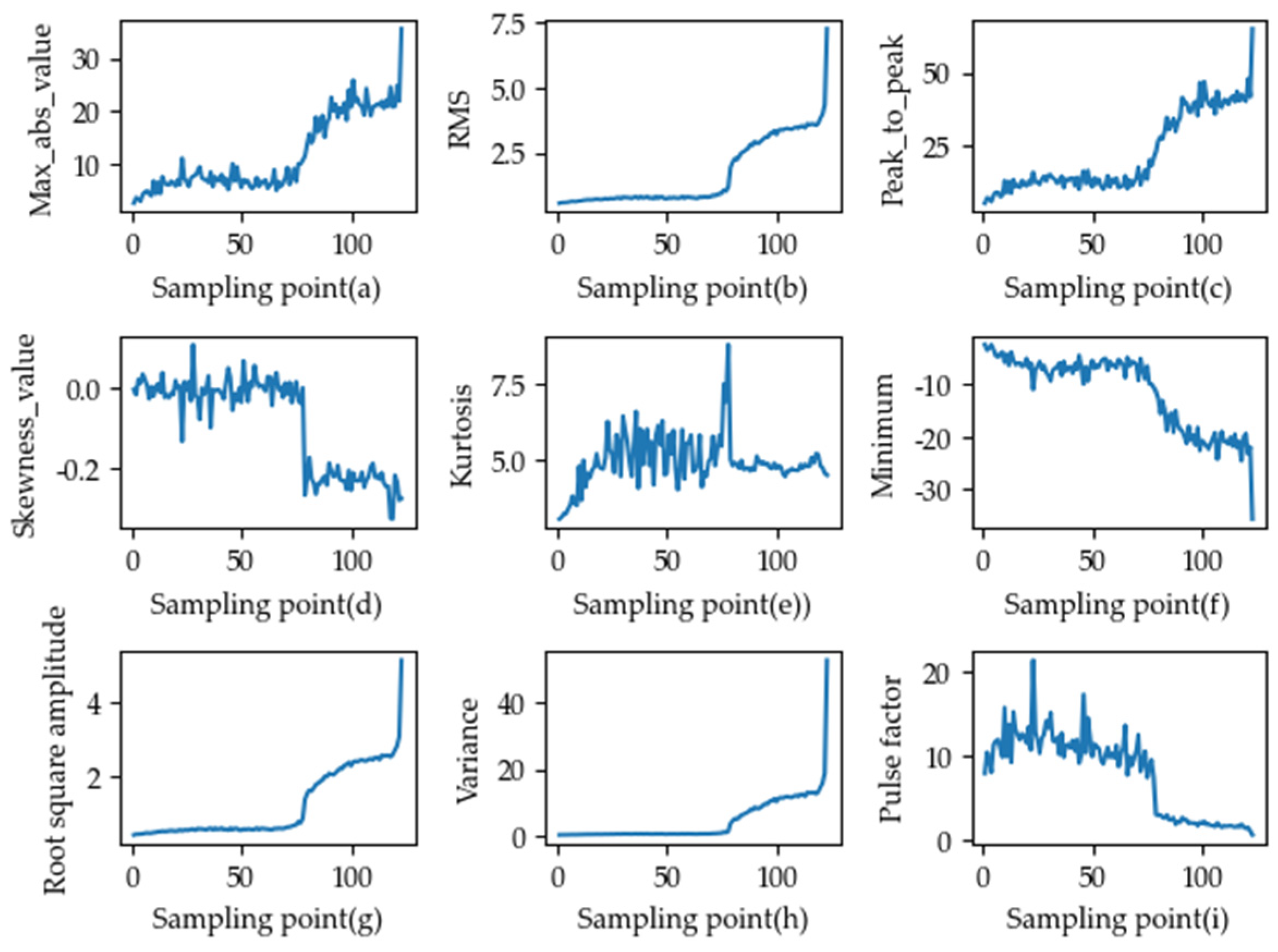
To establish the potential effectiveness of this design, our study uses the public bearing dataset provided by Xi’an Jiaotong University. This dataset encompasses vibration signals collected from 15 bearings over their entire life cycle and across three distinct operating conditions. Bearing 1-1 comprises a total of 123 tables, each containing 32,768 sampling points at a frequency of 25.6 kHz and an interval of 1 min. Each sampling period has a duration of 1.28 s. During the training phase, multiple feature values are extracted from data contained in the 123 tables. These values consist of diverse time-domain features of the vibration signals observed across the complete life cycle, as demonstrated in Figure 3.

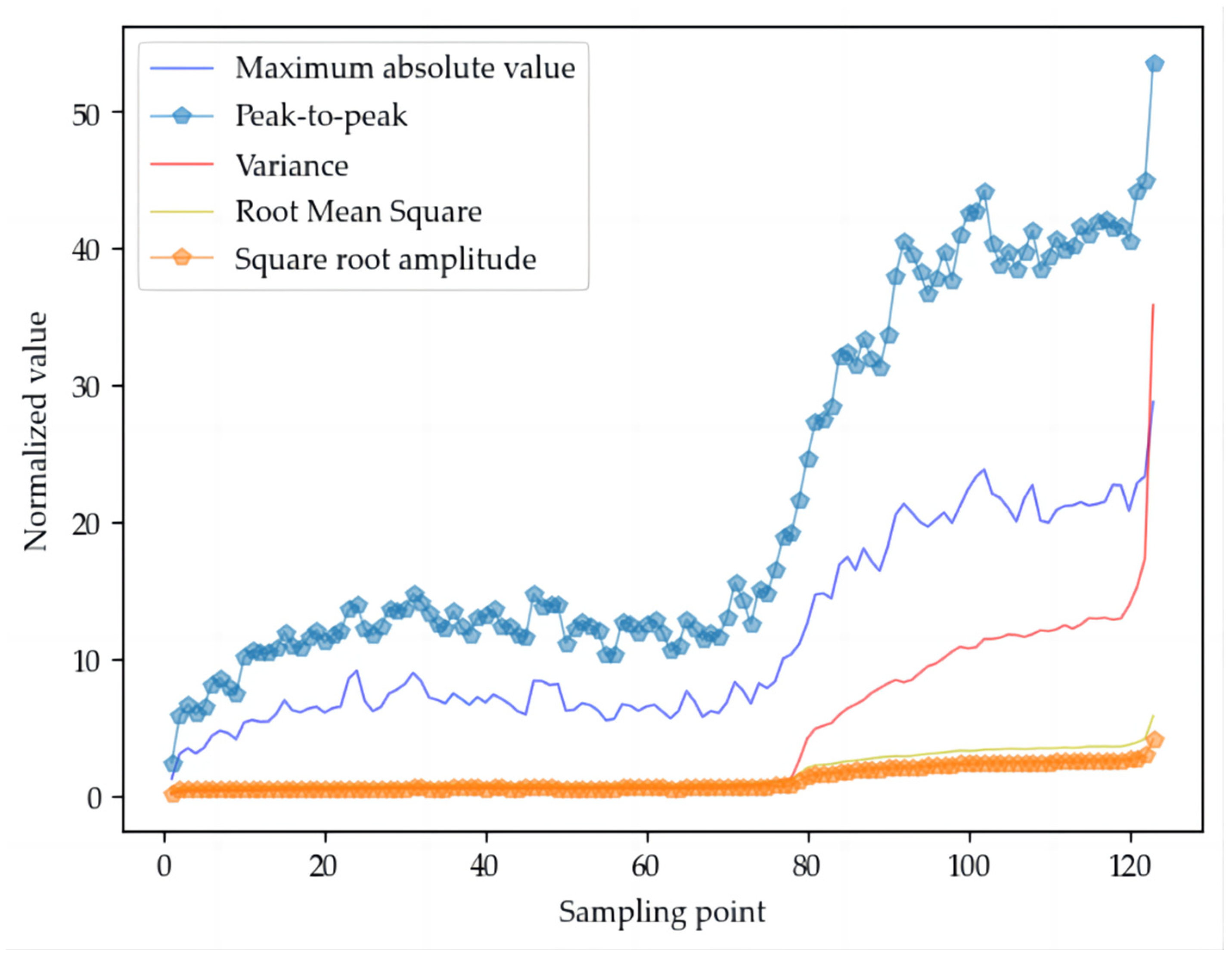
After setting the rising label y, we input F into the L1 regularization model for matching with the label; a time-domain feature map of the bearing with a rising trend was obtained, as shown in Figure 4.

The algorithm captures the features, which consistently lead to HI construction, as shown in Figure 4. The first 70% of the data are fed into the model, and the steps from Algorithm 1 are followed to train the MTBWO-BiGRU model. The second 30% validation set is used as the true values for validation, and the error of the model is calculated. In order to prove the goodness of fit of this model, we compared the results between the popular BiGRU [17] and BiLSTM [18] models and the MTBWO-BiGRU model. To ensure objectivity and fairness, all models are configured identically in terms of the number of hidden layers, the number of neurons, the learning rate, the activation function (tanh), the step size and the batch size. After using MTBWOA to establish the best parameters, we found that the parameters listed below in

Table 2. BiGRU and BiLSTM model parameters.

Parameter	Parameter Value
Layers	2
Cells	32
Batch Size	256
Learning Rate	0.001
Step	1

worked best.

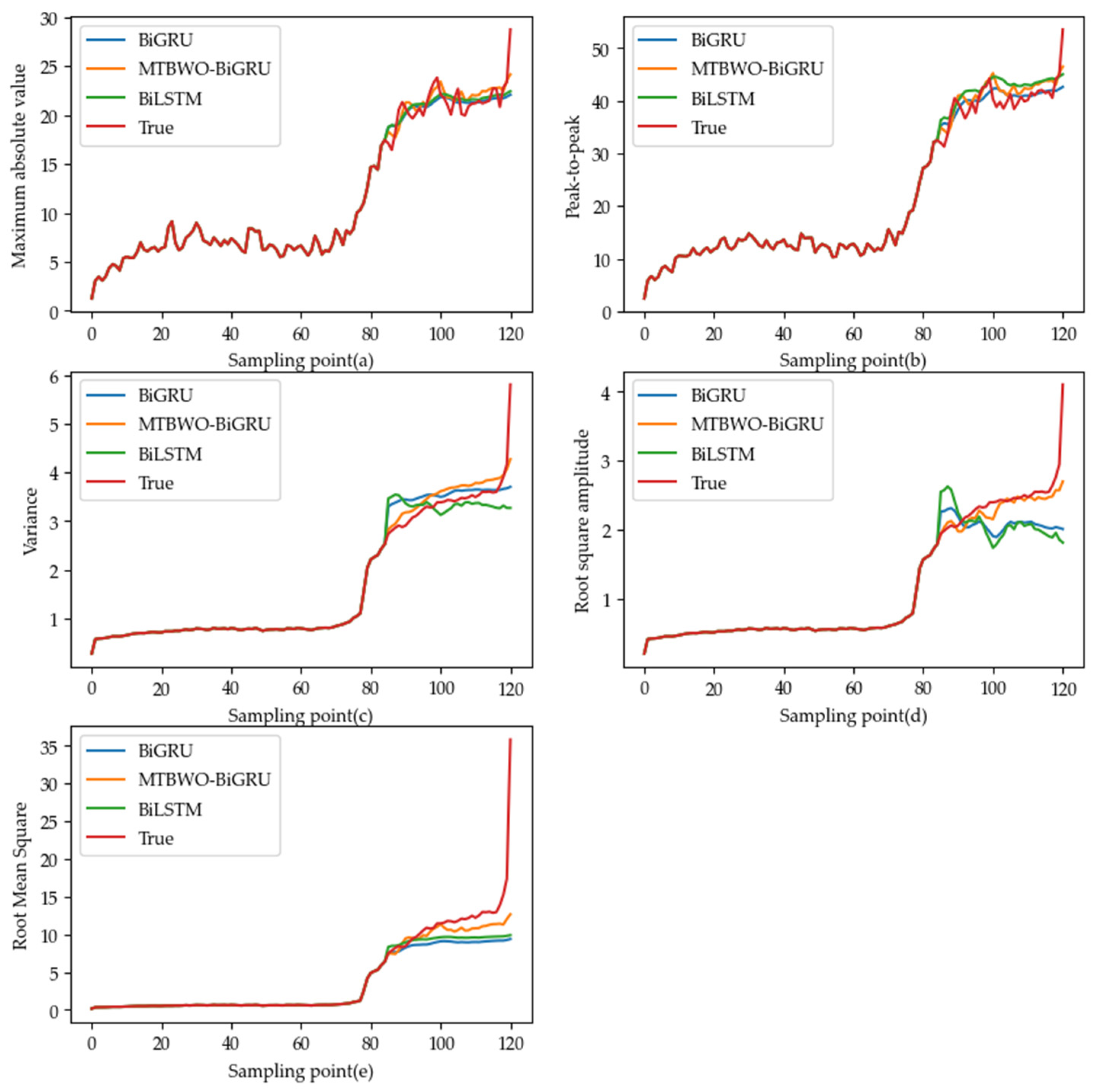
Since the Bray–Curtis distance formula used in the HI formula already contains the normalization effect, we performed inverse normalization by using the mean and variance after making the prediction to rescale the eigenvalues to their initial proportions. The first 70% of the data are all the same, indicated in red, and the next 30% of the predicted data are compared using MTBWO-BiRGU, BiGRU and BiLSTM, with different colored lines for differentiation, and the obtained predictions are shown in Figure 5a–e.

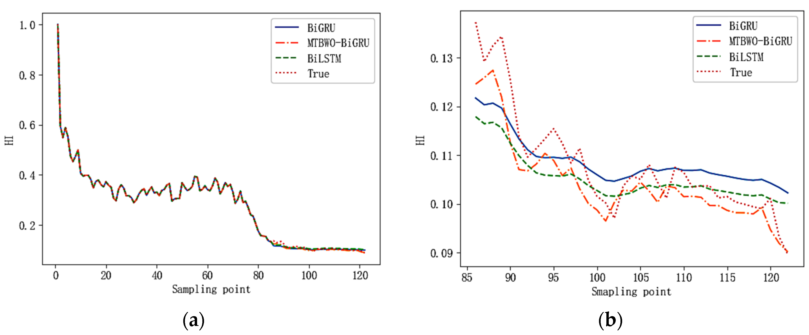
Since the bearing is healthy in the initial state, we record the eigenvalues of the first time window as healthy features. With Algorithm 2, the health features extracted from the first time window and the degradation features of the bearings are utilized to create the HI curve. The first 70% of the data are referred to as the ground truth, while the remaining 30% of the data, ranging from the 85th to the 123rd data point, are employed as validation data input to the BiGRU, BiLSTM and MTBWO-BiGRU models for comparison. The simulated comparison results are illustrated in Figure 6. To aid visualization, we set the results for the different models in four different colors.

Figure 6a shows the value progressively decreasing to around 0.3, where it stabilizes.

Subsequently, a substantial decrease occurs until it reaches 0. Due to the slight differences between the data points, discerning the pattern from the plot may prove challenging. Hence, the subsequent graph in Figure 6b enlarges the inspection of the validation data from the 85th to the 123rd data point to provide a more thorough comparison. It can be seen that the BiGRU model is the best fit to the actual curve, and the performance of BiGRU is optimal when other model parameters are constant, which verifies the superiority of the BiGRU model.

4.2. Actual Data Test

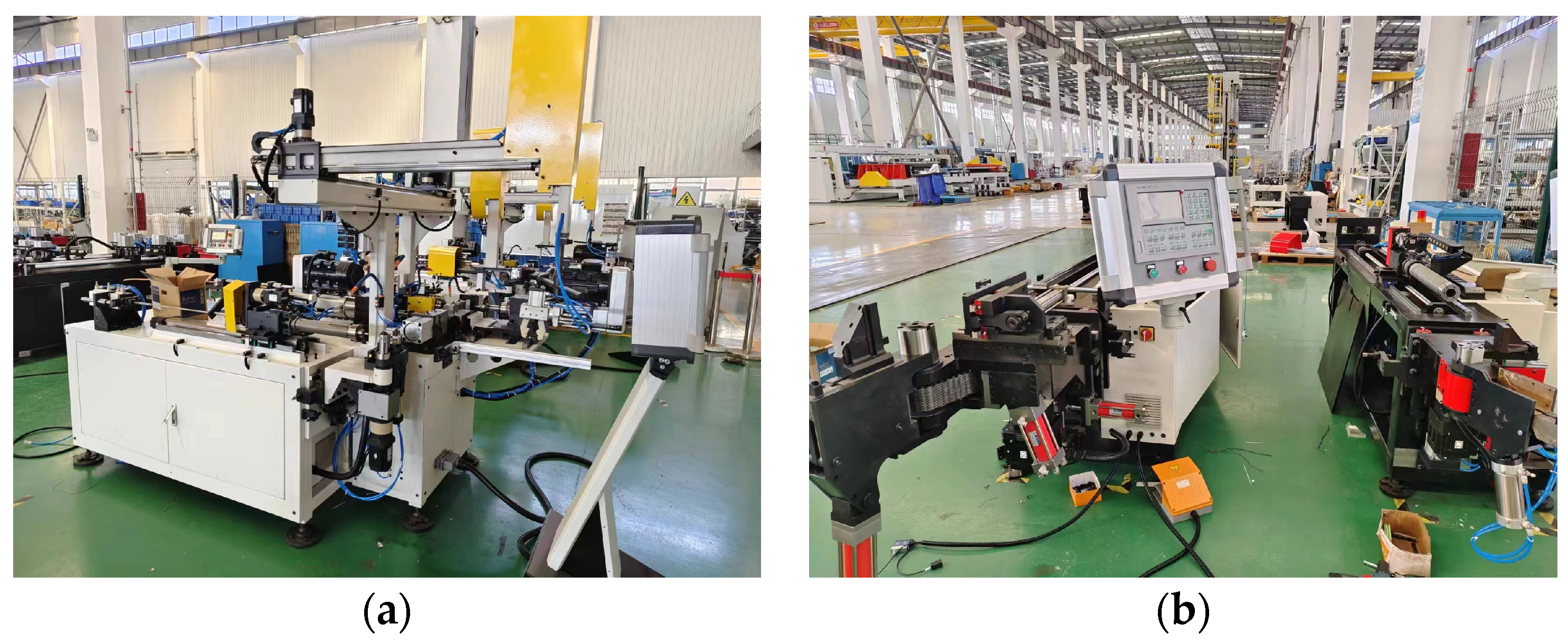
After conducting training and testing on a publicly available dataset, the models underwent further validation using actual data acquired from SMT Corporation. The equipment site is shown in Figure 7a,b.

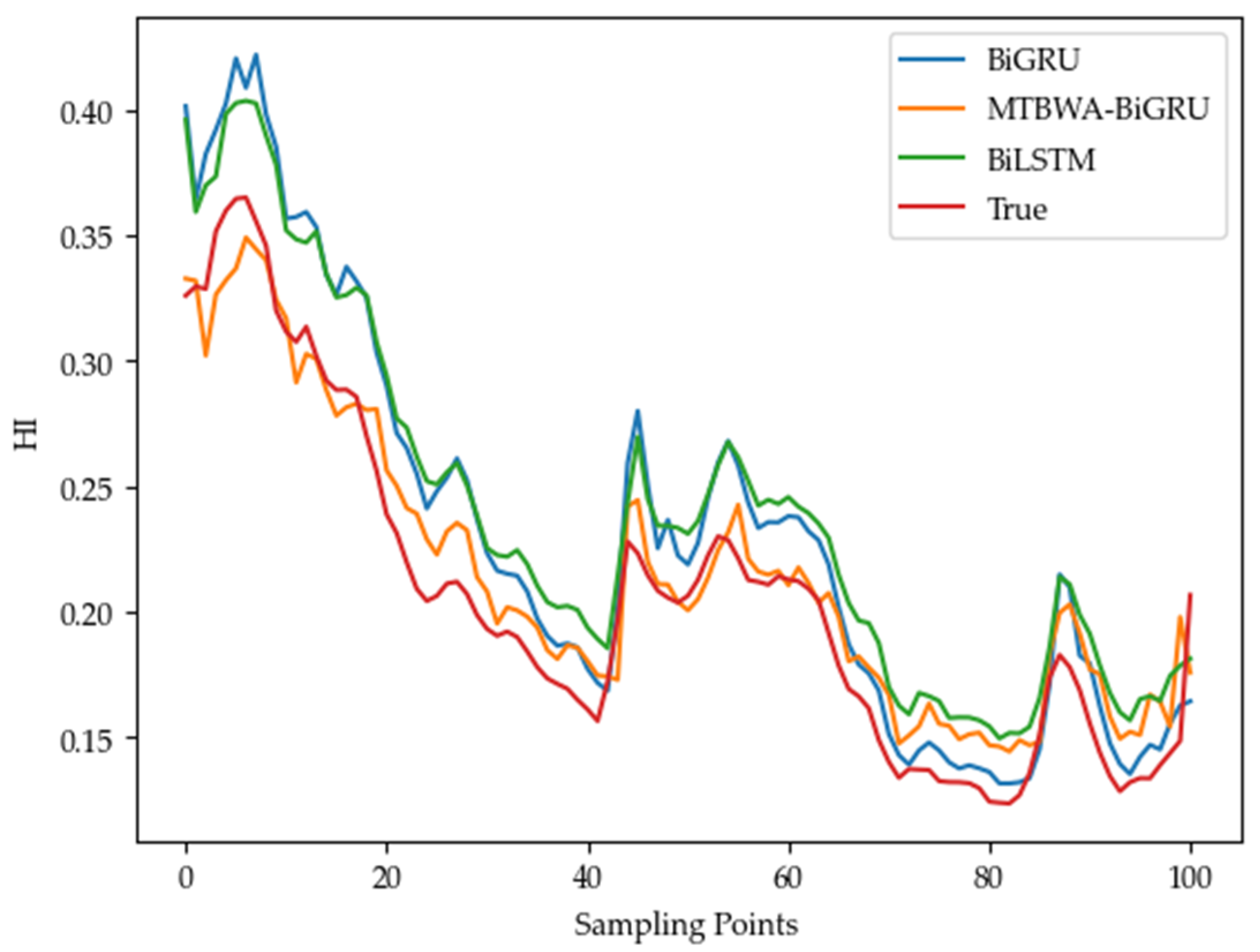
The data are gathered at a sampling frequency of 12.8 kHz, and each file contains 4096 data points. A total of 300 files are at our disposal, whereby the initial 200 files are designated for training, and the remaining 100 files are designated for validation. The resulting comparison plot for HI degradation can be seen in Figure 8.

$$\mathrm{rate}=\frac{\mathrm{data}\left[\mathrm{i}\right]-\mathrm{data}\left[\mathrm{i}-1\right]}{\mathrm{data}\left[\mathrm{i}-1\right]}$$

(6)

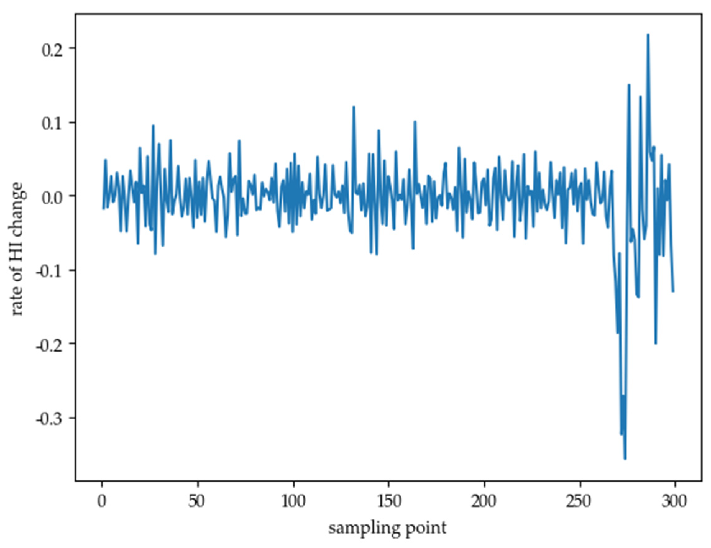
To detect faults in bearings, the utilization of the rate of change is employed. The calculation of the rate of change in the HI is based on degradation data from the HI curve obtained through actual measurements. Equation (6), as shown in Figure 9, was used to calculate the rate of change in the HI.

The data revealed that the rate of change exhibited fluctuation within a narrow range of approximately 0.1 initially. However, there was a sudden increase in the negative direction to −0.18 at the 270th data point, followed by continuous intense fluctuations. This observation leads to the conclusion that the bearing develops a fault at this point. The threshold for the rate of change can be set in such manner that exceeding the threshold indicates bearing failure [19,20,21].

When a bearing is in normal operation, its vibration signal usually shows a certain stability and regularity. However, once a bearing failure occurs, such as damage to the inner ring, outer ring or rolling element, it will lead to a sudden change in the characteristics of the vibration signal. This change is often accompanied by a sudden increase in the rate of change in the vibration signal, i.e., the rate of change in the vibration signal is much higher than the rate of change under normal operating conditions.

Therefore, signs of bearing failure [22] can be detected in time by monitoring the rate of change in the vibration signal.

4.3. Experimental Discussion and Analysis

4.3.1. Error Comparison

The model error was calculated using Equations (7) and (8).

(1)

RMSE

$$\mathrm{RMSE}=\sqrt{\frac{1}{\mathrm{n}}{\displaystyle \sum _{\mathrm{i}=1}^{\mathrm{n}}{\left({\mathrm{y}}_{\mathrm{i}}- {\hat{\mathrm{y}}}_{\mathrm{i}}\right)}^2}}$$

(7)

(2)

MAE

$$\mathrm{MAE}=\frac{1}{\mathrm{n}}{\displaystyle \sum _{\mathrm{i}=1}^{\mathrm{n}}\left|{\overline{\mathrm{y}}}_{\mathrm{i}}{-\mathrm{y}}_{\mathrm{i}}\right|}$$

(8)

The errors for the three models were compared using the aforementioned two equations, as shown in

Table 3. Error comparison table between MTBWO-BiGRU, BiLSTM and BiGRU.

Model	RMSE	MAE
MTBWO-BiGRU	2.284015	1.0631934
BiLSTM	2.829135	1.5084976
BiGRU	2.7955768	1.4016339

.

4.3.2. Speed Comparison

In order to compare the speed of each model iteration, the start time command is added at the beginning of the iteration, and the end time command is added at the end of the iteration, and the difference between the two is used as the speed of the iteration. The results are shown in

Table 4. Speed comparison between MTBWO-BiGRU, BiLSTM and BiGRU.

Model	Speed
MTBWO-BiGRU	0.220 s
BiLSTM	0.229 s
BiGRU	0.230 s

.

4.3.3. Accuracy Comparison

In order to compare the accuracy of each model, the accuracy of the model was calculated using Equation (9).

$$\mathrm{r}\_\mathrm{squared}=1-\frac{{\left(\mathrm{pred}-\mathrm{true}\right)}^2}{{\left(\mathrm{pred}+\mathrm{true}\right)}^2}$$

(9)

According to Equation (9), the accuracy of the MTBWO-BiGRU model is 92.57%. The accuracy of the BiLSTM model is 70.68%, and the accuracy of the BiLSTM-Attention model is 76.32%.

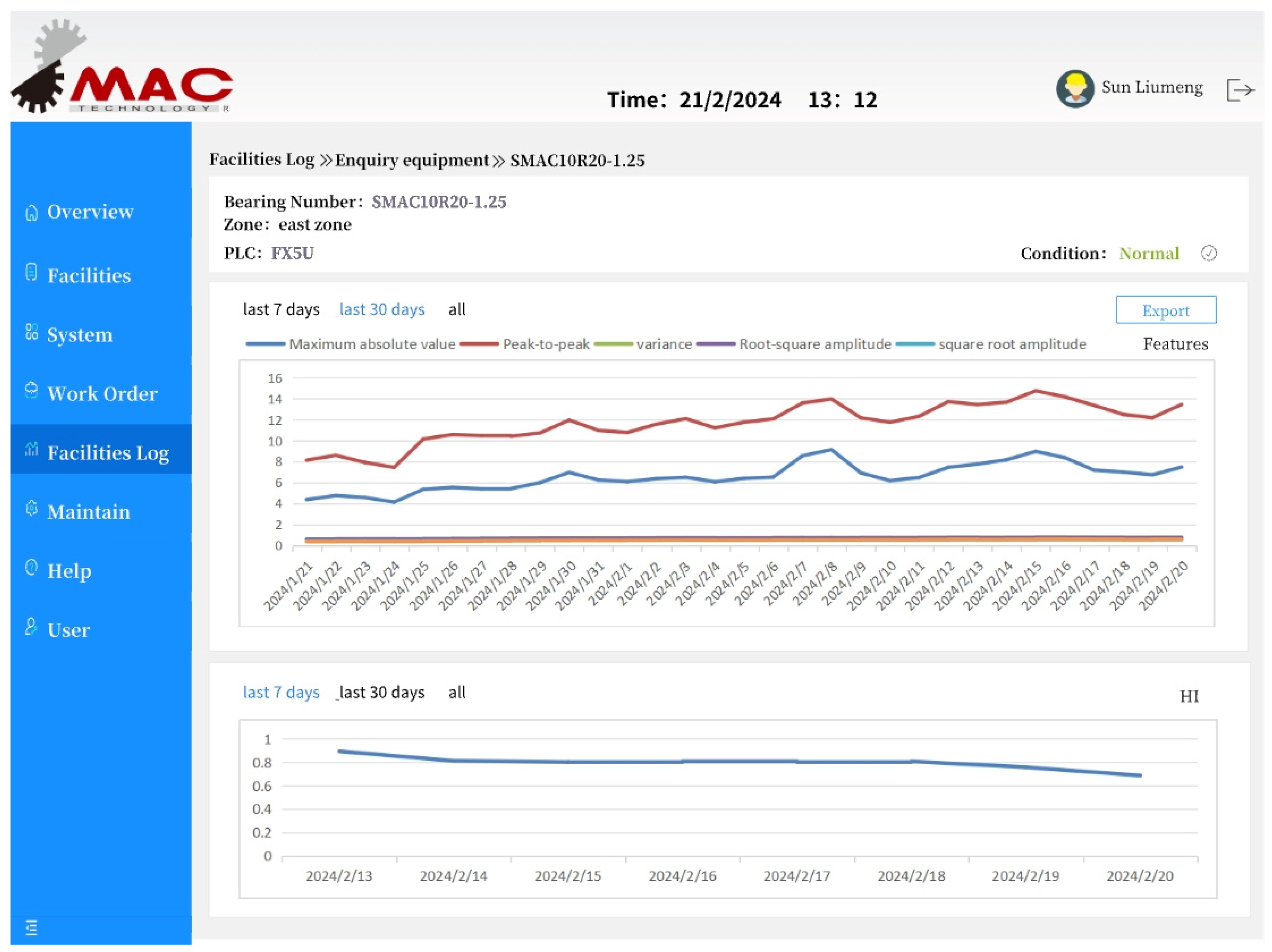
4.4. Cloud Platform Testing

The Mitsubishi FX5U was tested in practice to apply this system. To ensure accurate data collection, it is recommended for the characteristic information to be recorded at the beginning of the bearing’s use and to upload the vibration data sequence once a day. To monitor the status of the bearings, it is necessary to log into the physical control platform. The PC terminal monitoring platform interface is shown in Figure 10.

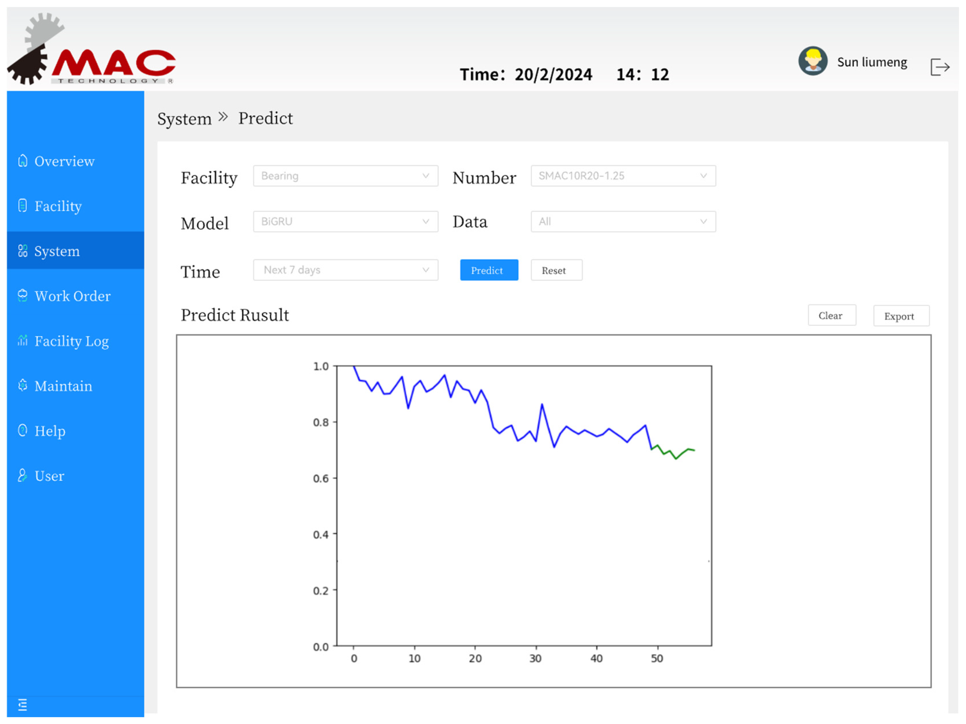
To make a prediction, it is necessary to open the prediction module and select the device, training model, training data and prediction duration. When one clicks on the prediction button, the HTML will request form information from the server. To predict the data for the next 7 days, all past data must be selected. The blue line represents the historical data section, and the green line represents the predicted data section, as shown in Figure 11.

5. Discussion

Below, we discuss our main findings based on the experimental results in the previous section in terms of training errors, runtime and accuracy, as follows.

5.1. Training Errors

The training error is a key indicator of how well the model fits the training data during the learning process, and its magnitude directly reflects the model’s ability to fit the training data.

This study aimed to explore the performance of different models in specific tasks, and during the comparison process, as shown in Table 3, it can be seen that the RMSE and MAE of the MTBWO-BiGRU model have significant advantages compared to BiLSTM and BiLSTM-Attention. This is due to the fact that controlling the flow of information through the update gate and reset gate effectively avoids the long-term dependency problem and mitigates the effects of gradient vanishing and gradient explosion, which enables the model to better capture the important features in the sequence data and effectively control the transmission and retention of key information.

5.2. Runtime

In the comparison process, as shown in Table 4, we found that the shortest iteration time was demonstrated for the MTBWO-BiGRU model. Although the difference in time per round is not substantial, this time gap grows larger as more and more rounds are iterated. GRUs typically have fewer parameters than LSTMs. The simplified structure of GRUs may make the model more parametrically efficient, allowing the network to learn faster and potentially generalize better with fewer data, and they may converge faster during training and be less prone to overfitting, which can be particularly beneficial in situations where the amount of training data is limited.

5.3. Accuracy

Through the use of Equation (9), we were able to clearly compare the accuracy of MTBWO-BiGRU with BiGRU and BiLSTM. The reduced complexity of GRUs may make them less prone to overfitting, especially with limited training data. BiGRUs may generalize better to unseen data, thus improving accuracy. Additionally, the MTBWO algorithm makes the hyperparameters of BiGRU reach the optimal values, so that the model effect performs well.

6. Conclusions

The current study presents the effectiveness of the MTBWO-BiGRU model with L1 regularization and the Bray–Curtis distance in constructing a health index for reliability prediction. This method was evaluated through both actual testing and simulation using the public bearing dataset provided by Xi’an Jiaotong University. It offers several advantages, particularly in the field of reliability prediction.

First, the collected data are sent to a Python deep-learning model running on a server for inference. This approach combines edge devices with cloud-focused deep-learning models, enabling real-time performance and minimizing energy consumption.

Second, the integration of advanced computer communication capabilities facilitates data transfer to the application layer. The cloud monitoring platform continuously monitors the health indicators of bearings in real time while maintaining a threshold for the rate of change. When the threshold is exceeded, the platform triggers an alarm, alerting personnel to carry out maintenance.

Lastly, this article introduces a new bio-inspired metaheuristic algorithm called the MTBWOA, which draws inspiration from the mating behavior of black widow spiders and further enhances the BWO algorithm. By incorporating multi-objective optimization and time-varying iteration arrays, the algorithm can optimize multiple parameters while optimizing the hyperparameters in the BiGRU model. This reduces iteration time, improves efficiency and enables faster convergence. Experimental results demonstrate that the MTBWO-BiGRU model achieves an accuracy of 92.57%, surpassing that of BiLSTM and BiGRU, highlighting the superiority of the proposed approach.

Implementing this approach can significantly mitigate the detrimental effects of machine wear and tear, leading to a reduction in downtime and improved efficiency in industrial operations. Furthermore, it promotes industrial automation and intelligence. However, our study still has some limitations. In future investigations, we plan to focus on examining additional productive temporary and spectral feature values. We also aim to expand the ability to predict the lifespan of various component types, enabling more precise monitoring of the health condition of industrial equipment.

References

- Wan, S.; Li, T.; Fang, B.; Yan, K.; Hong, J.; Li, X. Bearing Fault Diagnosis Based on Multisensor Information Coupling and Attentional Feature Fusion. IEEE Trans. Instrum. Meas. 2023, 72, 3514412. [Google Scholar] [CrossRef]
- Duan, R.; Liao, Y.; Yang, L.; Song, E. Faulty Bearing Signal Analysis With Empirical Morphological Undecimated Wavelet. IEEE Trans. Instrum. Meas. 2022, 71, 3508711. [Google Scholar] [CrossRef]
- Yang, Y.; Liu, H.; Han, L.; Gao, P. A Feature Extraction Method Using VMD and Improved Envelope Spectrum Entropy for Rolling Bearing Fault Diagnosis. IEEE Sens. J. 2023, 23, 3848–3858. [Google Scholar] [CrossRef]
- Xue, L.; Ningyun, L.; Chuang, C.; Tianzhen, H.; Bin, J. Attention mechanism based multi-scale feature extraction of bearing fault diagnosis. J. Syst. Eng. Electron. 2023, 34, 1359–1367. [Google Scholar] [CrossRef]
- Liu, X.; Xia, L.; Shi, J.; Zhang, L.; Bai, L.; Wang, S. A Fault Diagnosis Method of Rolling Bearing Based on Improved Recurrence Plot and Convolutional Neural Network. IEEE Sens. J. 2023, 23, 10767–10775. [Google Scholar] [CrossRef]
- Zhao, Z.; Du, Z.; Yang, K.; Sun, H.; Wei, J.; Liu, Y. A Data-Driven Model for Bearing Remaining Useful Life Prediction with Multi-step Long Short-Term Memory Network. In Signal and Information Processing, Networking and Computers; Lecture Notes in Electrical Engineering; Springer: Singapore, 2023; Volume 917, pp. 1129–1138. [Google Scholar]
- Zou, K.; Yuan, H.; Wang, H. Rolling Bearing Fault Prediction Based on Feature Fusion of HI Curves and GRU Networks. In Proceedings of the 2023 38th Youth Academic Annual Conference of Chinese Association of Automation (YAC), Hefei, China, 27–29 August 2023; pp. 469–474. [Google Scholar] [CrossRef]
- Ni, Q.; Ji, J.C.; Feng, K. Data-Driven Prognostic Scheme for Bearings Based on a Novel Health Indicator and Gated Recurrent Unit Network. IEEE Trans. Ind. Inform. 2023, 19, 1301–1311. [Google Scholar] [CrossRef]
- Wang, H.; Zhang, X.; Guo, X.; Lin, T.; Song, L. Remaining useful life prediction of bearings based on multiple-feature fusion health indicator and weighted temporal convolution network. Meas. Sci. Technol. 2022, 33, 104003. [Google Scholar] [CrossRef]
- Yang, C.; Ma, J.; Wang, X.; Li, X.; Li, Z.; Luo, T. A novel based-performance degradation indicator RUL prediction model and its application in rolling bearing. ISA Trans. 2022, 121, 349–364. [Google Scholar] [CrossRef] [PubMed]
- He, M.; Guo, W. An Integrated Approach for Bearing Health Indicator and Stage Division Using Improved Gaussian Mixture Model and Confidence Value. IEEE Trans. Ind. Inform. 2022, 18, 5219–5230. [Google Scholar] [CrossRef]
- Buccafurri, F.; de Angelis, V.; Lazzaro, S. MQTT-A: A Broker-Bridging P2P Architecture to Achieve Anonymity in MQTT. IEEE Internet Things J. 2023, 10, 15443–15463. [Google Scholar] [CrossRef]
- He, L.; Wu, H.; Wen, X.; You, J. Seismic Acoustic Impedance Inversion Using Reweighted L1-Norm Sparse Constraint. IEEE Geosci. Remote Sens. Lett. 2022, 19, 8027105. [Google Scholar] [CrossRef]
- Yan, X.; Liang, W.; Xu, D. Remaining Useful Life Interval Prediction for Complex System Based on BiGRU Optimized by Log-Norm. IEEE Access 2022, 10, 108089–108102. [Google Scholar] [CrossRef]
- Xu, D.; Yin, J. An Improved Black Widow Optimization Algorithm for Engineering Constrained Optimization Problems. IEEE Access 2023, 11, 32476–32495. [Google Scholar] [CrossRef]
- Keleş, M.K.; Kiliç, Ü. Binary Black Widow Optimization Approach for Feature Selection. IEEE Access 2022, 10, 95936–95948. [Google Scholar] [CrossRef]
- Zhang, C.; Wang, D.; Wang, L.; Song, J.; Liu, S.; Li, J.; Guan, L.; Liu, Z.; Zhang, M. Temporal data-driven failure prognostics using BiGRU for optical networks. J. Opt. Commun. Netw. 2020, 12, 277–287. [Google Scholar] [CrossRef]
- Wang, S. A Stock Price Prediction Method Based on BiLSTM and Improved Transformer. IEEE Accesss 2023, 11, 104211–104223. [Google Scholar] [CrossRef]
- Tang, M.; Liao, Y.; Duan, R.; Xue, J.; Zhang, X. Bearing Fault Diagnosis Based on the Maximum Squared-Enveloped Multipoint Kurtosis Morphological Deconvolution. IEEE Trans. Instrum. Meas. 2022, 71, 3509711. [Google Scholar] [CrossRef]
- Song, X.; Liao, Z.; Jia, B.; Kong, D.; Niu, J. Rolling Bearing Fault Diagnosis Under Different Severity Based on Statistics Detection Index and Canonical Discriminant Analysis. IEEE Access 2023, 11, 86686–86696. [Google Scholar] [CrossRef]
- Chen, X.; Yang, R.; Xue, Y.; Huang, M.; Ferrero, R.; Wang, Z. Deep Transfer Learning for Bearing Fault Diagnosis: A Systematic Review Since 2016. IEEE Trans. Instrum. Meas. 2023, 72, 3508221. [Google Scholar] [CrossRef]
- Zhang, W.; Chen, D.; Xiao, Y.; Yin, H. Semi-Supervised Contrast Learning Based on Multiscale Attention and Multitarget Contrast Learning for Bearing Fault Diagnosis. IEEE Trans. Ind. Inform. 2023, 19, 10056–10068. [Google Scholar] [CrossRef]
Figure 1.
System framework diagram.
Figure 2.
System architecture diagram.
Figure 3.
Full-cycle vibration signal time-domain characteristics of Bearing 1-1: (a) shows the maximum absolute value of the vibration signal; (b) shows the RMS; (c) shows the peak-to-peak; (d) shows the skewness; (e) shows the kurtosis; (f) shows the minimum; (g) shows the RA; (h) shows the variance; and (i) shows the pulse factor.
Figure 4.
Bearing 1-1 characteristics chart with an upward trend.
Figure 5.
Comparison of predicted values of features under the three models: (a) shows the comparison of the maximum absolute value; (b) shows the comparison of the peak-to-peak; (c) shows the comparison of the variance; (d) shows the comparison of the root square amplitude and (e) shows the the comparison of the root mean square.
Figure 6.
BiGRU, BiLSTM and MTBWO-BiGRU model effect comparison chart. (a) illustrates that the HI model accurately depicts the bearing degradation process, and (b) enlarges the inspection of the validation data from the 85th to the 123rd data point to provide a more thorough comparison.
Figure 7.
On-site equipment diagram. Panel (a) shows the bearing in the equipment. Panel (b) shows the terminal control system.
Figure 8.
Comparison of the effect of the HI with the measured data under the three models.
Figure 9.
Bearing HI rate of change chart.
Figure 10.
Terminal monitoring page. In the above figure, the blue line represents maximum absolute value, the red line represents peak-to peak, the green line represents variance, the purple line represents root-square amplitude,the light blue line represents square root amplitude.
Figure 11.
Display diagram of the monitoring platform prediction module.