Abstract
A structured mesh generation method based on an improved ray-tracing technique is proposed for finite time difference domain (FDTD) simulation in this paper. This method converts the triangular faces provided by the STL file into the structured mesh required by the FDTD method. The size of the generated structured mesh is determined by the size of the triangular element, so it is non-uniform and can adapt to the shape of the target. In addition, this method proposes an improved ray-tracing technique to avoid the singularities of the object, so it has much better accuracy than the conventional method. Two representative electromagnetic objects, an Su-30 aircraft and a complex bow-tie antenna, representing a typical electrically large model and fine structure, respectively, are used to validate the accuracy of the mesh generation method. The results show that the presented method has high accuracy, regardless of whether it is used for large targets or fine structures such as a small hole, strip, thin layer, etc.
1. Introduction
The finite difference time domain (FDTD) method is one of the major numerical calculation methods used to analyze electromagnetic problems by solving Maxwell’s differential equations. Before using the FDTD method to analyze electromagnetic problems, the space needs to be discretized into cuboid elements called Yee cells [1]. The quality of a Yee cell has a great influence on the calculation accuracy and efficiency of the FDTD method. A large number of mesh generation methods have been proposed for generating Yee cells [2,3,4,5,6,7,8,9]. A three-dimensional (3D) automatic FDTD mesh generation scheme was put forward in 1993, which provided a relatively complex process of 3D mesh generation [2]. In 2000, a non-uniform conforming mesh generator was designed for the accurate modeling of smooth curved surfaces [3]. In 2004, a three-dimensional CAD-based mesh generator that had improved capabilities for 3D arbitrary geometries was presented [4]. A three-dimensional sub-gridding algorithm for the FDTD method was presented by Michal Okoniewsk [5], which provided a smooth transition between the coarse and fine meshes. G. Junkin presented a mesh generation for a locally conformal FDTD Dey–Mittra algorithm that evolved from a universal structured grid [6], etc. Richard Holland used conformal meshing techniques to improve computing efficiency [10]. Chen Wu, etc., described a circular mesh scheme for the non-orthogonal finite difference time domain method [11].
Although there are currently many mesh generation methods, these methods are either not adaptive both for electrically large models and fine structures, or are computationally complex and difficult to implement. This paper presents a simple structured mesh generation method based on an improved ray-tracing technique to avoid such problems. The input file of this method is an STL file, which is a commonly used format in many graphics software, such as Solidworks, CAD, etc. The STL file contains triangular face information of the object. The proposed method transforms the triangular element into a structured mesh by using an improved ray-tracing technique. The mesh size can be adaptively modified according to the size of the triangular element. So, it can reasonably determine the size of the grid according to the structure of the object, thereby ensuring the computational accuracy and efficiency of the FDTD algorithm.
This paper provides the completion process of the mesh generation method. It first generates a non-uniform structured mesh in the entire computation domain, then recognizes the structured mesh on the surface of the object, and finally recognizes the internal structured mesh in the object. At last, it uses two representative electromagnetic objects, an Su-30 aircraft and a complex bow-tie antenna, representing a typical electrically large model and fine structure, to validate the accuracy of the mesh generation method by comparing the results with those of the CST software. It shows that the presented method has high accuracy, regardless of whether it is used to subdivide a large target or small hole, strip, thin layer, etc.
2. Methods
The mesh generation method presented in this paper is based on the STL format file, which fits the target by using the surface triangular element, as shown in Figure 1a. The STL format file contains smaller memory compared with other 3D general file formats such as STEP, IGES, VDA-FS, and so on. It is an ideal file format used to generate a mesh for the FDTD method. The whole model’s surface is divided by a set of triangles and then exported as an STL file by modeling software. The STL file format is shown in Figure 2. The STL file starts with the model’s name. Next, each triangle element is described with its facet’s normal vector and vertex coordinates. Different triangles are divided by “endfacet”. When all triangle elements are recorded completely, the STL file ends with the model’s name. The STL file can be obtained directly from commercial software such as CAD, Solidworks, etc. These triangular elements need to be transformed into a structured mesh such as that shown in Figure 1b in order to satisfy the requirement of the FDTD method.
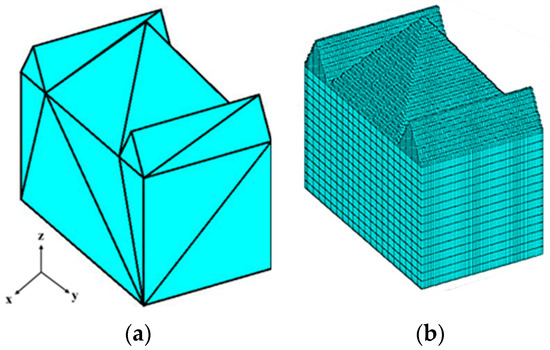
Figure 1.
Grid structure of an object. (a) Surface triangular element. (b) Structured mesh.
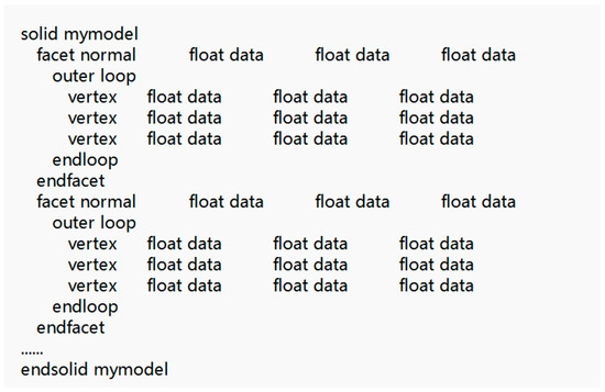
Figure 2.
The STL file format.
The mesh generation method contains three steps: (1) generate a non-uniform structured mesh in the whole computation domain; (2) recognize the structured mesh on the surface of the object; (3) recognize the internal structured mesh in the object.
2.1. Generate Non-Uniform Structured Mesh
As is known, a uniform mesh is easy, but not suitable for electromagnetic targets that include both fine and large structures. The small mesh used to fit the fine structures results in large number of cells in the whole computation domain, which not only needs huge computer memory but also greatly increases the computing time. On the contrary, a non-uniform mesh, which uses a small mesh in the fine structure and large mesh in the rough structure, can greatly reduce the number of cells. So, this paper proposes a non-uniform gridline generation method.
The specific process is as follows. First, it generates uniform gridlines in the whole computation domain. To fully adapt to the physical characteristics of the model, the vertex coordinates recorded in the STL file are used to help generate mesh lines. According to the discretization requirement of the FDTD algorithm, the maximum mesh size needs to be less than ; here, is the minimum wavelength of the frequency band. Therefore, it divides the computational space into uniform grids with a size of , as shown by the dotted line in Figure 3. Second, it refines the uniform grid lines according to the size of the surface triangular elements. When the object includes a fine structure, grid lines may be too rough to fit the target well. A mesh may cross a whole triangular element, such as that shown by triangle 2 and triangle 3 in Figure 3. In this case, a new grid line will be added in the original rough mesh, as shown by grid line a and grid line b in Figure 3. In most cases, optimizing the grid line only once is not enough. For example, in Figure 3, triangle 3 is still included in one mesh. So, it needs to refine the grid lines continuously (adding line c) until all the triangles are subdivided by at least two meshes. By using this method, the entire computation domain can be discretized into a non-uniform structured mesh.
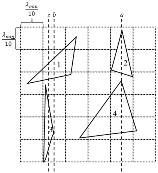
Figure 3.
Refine the uniform grid lines according to the size of the triangular element.
2.2. Recognize Surface Structured Mesh of Object
The structured mesh generated above covers the entire computation domain, including both object and non-object areas. It needs to recognize these structured meshes of the object in order to assign the medium parameters of the object to these meshes. Because the STL file only records the facet information of the object, it recognizes the surface structured mesh of the object first by using the projection method. Taking one triangle element as an example, the method is as follows:
- 1.
- Project the triangle element ABC onto the XOY plane and mark the projected triangle as A′ B′ C′, as shown in Figure 4.
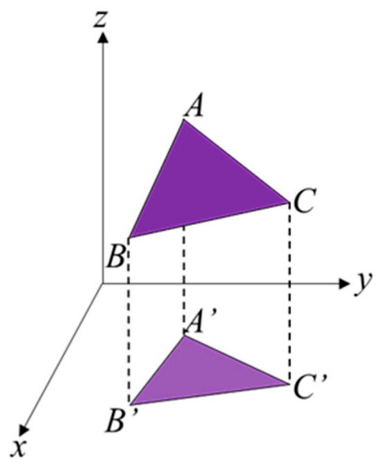 Figure 4. Triangle ABC and its projection A′ B′ C′.
- 2.
- Based on the vertex coordinates of triangle A′ B′ C′, determine the maximum value and minimum value in the X-direction and the maximum value and minimum value in the Y-direction. Based on these four values, a projected domain (the yellow domain in Figure 5) composed of many rectangular meshes that cover the triangle A′ B′ C′ totally can be obtained. The four vertex coordinates of the projected domain are recorded as (), (), (), (), respectively.
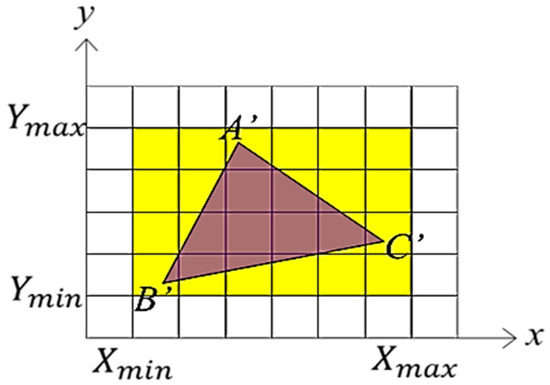 Figure 5. Projected rectangular area.
- 3.
- For all the rectangle meshes in the projected domain, the vector cross multiplication method is used to determine whether the mesh center point P is located inside A′ B′ C′. It first connects lines PA′, PB′, and PC′ and obtains three vectors , , and . It then calculates × , × and × . If the three cross product results are all positive or negative simultaneously, point P is located inside the projection triangle A′ B′ C′, as shown in Figure 6a. Otherwise, point P is located outside of the projection triangle A′ B′ C′, as shown in Figure 6b.
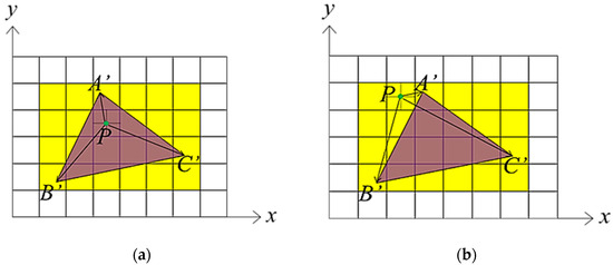 Figure 6. The location relationship between mesh center P and triangle A′ B′ C′. (a) Point P is located inside triangle A′ B′ C′. (b) Point P is located outside triangle A′ B′ C′.
- 4.
- For the point P that is located inside the projected triangle A′ B′ C′, it substitutes its projection coordinates (, ) to the plane equation of triangle ABC as follows:where , , are the vector components of the normal vector of triangle ABC in the X, Y and Z direction, respectively. (, , ) is the coordinate of an arbitrary point in triangle ABC. Then, , the z-coordinate of the projection point P′ in triangle ABC, as shown in Figure 7, can be solved. After that, the coordinate (, , ) of point P′ is determined; subsequently, the structured mesh including point P′ is recognized as the surface structured mesh of the object, as shown in Figure 8.
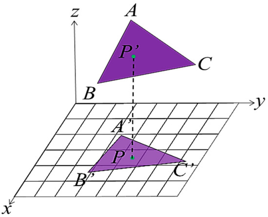 Figure 7. The intersection P′ of the triangle ABC.
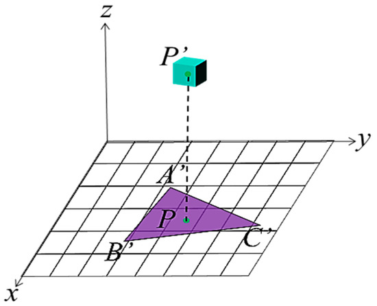 Figure 8. The mesh including point P′.
When all the triangular elements of the object are processed by using the projection method above, the object’s surface structured meshes can be recognized completely. Taking the model in Figure 1a as an example, after the surface mesh filling is completed, the result (sectional view) is as shown in Figure 9.
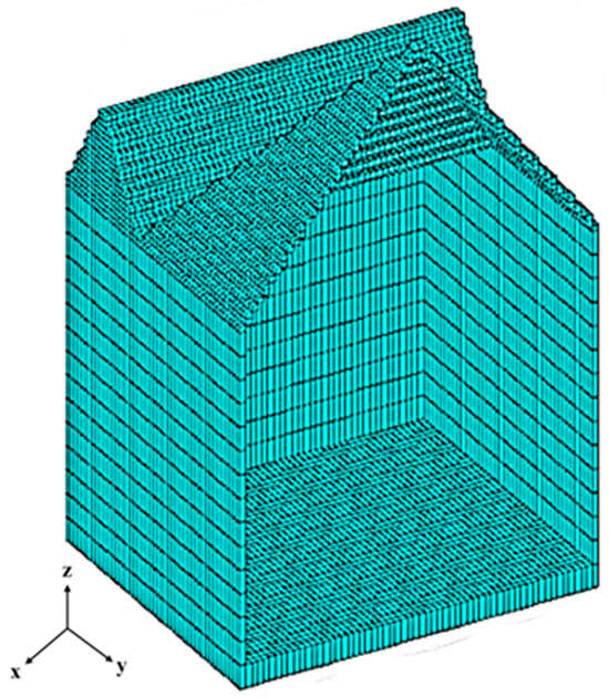
Figure 9.
The surface structured mesh of the object.
2.3. Recognize Internal Structured Mesh of Object
After the surface structured meshes of the object have been filled, the internal structured mesh in the object needs to be recognized. The ray tracing method is widely used to realize three-dimensional reconstruction, which can be used to judge the model area. Due to the complexity of the model, the conventional ray-tracing method has its disadvantages in dealing with the singularity problem, which causes significant errors. To avoid singularity and ensure the accuracy of recognition, an improved ray-tracing method is proposed in this paper.
The conventional ray-tracing method uses a number of intersection points to distinguish between the object area and non-object area. In this method, sufficient paralleled unidirectional rays pass through the object and leave intersection points on the surface of the object. For most cases, each ray penetrates the object and only forms two intersection points at the object’s surface. However, if the object is a multi-layered structure, as shown in Figure 10, the ray may form many intersection point pairs. For each point pair, the ray enters the object at the first intersection and then leaves the object at the second intersection. The entry point and the exit point exist in pairs. Therefore, it always has an even number of intersection points. For such cases, starting from the first entry point along the direction of ray emission, the part between the entry point 1 and its adjacent exit point 2 is recognized as the inner region of the object, as shown by the green part in Figure 10. The structured meshes in this area are recognized as the meshes of the object, while the part between exit point 2 and its adjacent next entry point 3 is recognized as the non-model region, as shown by the blank part in Figure 10. The structured meshes in this area are not the meshes of the object. So, repeatedly, all the structured meshes in the whole computation domain can be recognized.
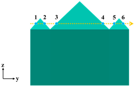
Figure 10.
Ray passing through multi-layer structures in one direction.
However, this method has difficulty dealing with the singularity problem. Singularity points are the special points formed by rays passing through the vertices of an object, as shown by point 1 and point 4 in Figure 11. In this figure, ray α passes through the object, leaving four points of intersection on the surface. It enters the object at point 2 and exits the object at point 3. Points 1 and 4 are singularity points that result in error in the judgment of the internal and external area of the object. According to the conventional ray-tracing method, the region between point 1 and point 2 will be falsely recognized as an object area, as will the region between point 3 and point 4. Meanwhile, the region between point 2 and point 3 will be falsely recognized as a non-object area. In fact, the region area between point 2 and point 3 is the object area while the rest belongs to the non-object area.
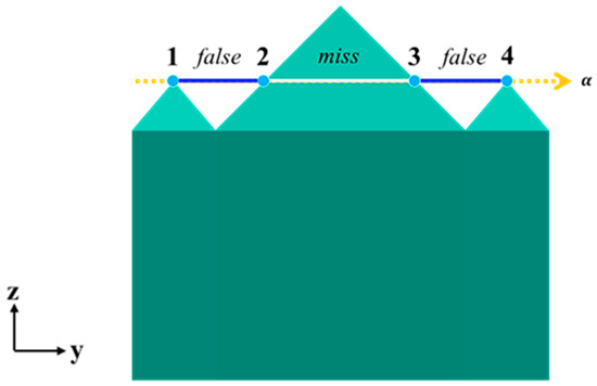
Figure 11.
Singularity problem in conventional ray-tracing method.
The best method to deal with such cases is to identify the singularity points and then delete them to avoid erroneous judgement. So, an improved ray-tracing method is proposed here. This method distinguishes real entry points and real exit points via a normal vector recorded by an STL file. It detects the vector angles between the normal vector of the triangle element where the point is located and the ray’s direction vector. If the angle is smaller than 90°, the ray exits the object at this point. If the angle is greater than 90°, the ray enters the object at this point. For a point that is a singularity point, it must be adjacent to different surfaces so it forms obtuse angles and acute angles simultaneously. As shown in Figure 12, ray α passes through the object. Point 1 is an intersection point that is on the intersecting line of two side surfaces, whose normal vector is shown by purple arrows in Figure 12. Its left surface’s normal vector forms with the ray α, while its right surface’s normal vector forms with the ray α. It can be seen from this figure that is smaller than 90° while is greater than 90°. The same applies to point 4. Thus, point 1 and point 4 are identified as singularity points. They will be deleted to avoid erroneous judgement. By using this method, when ray α passes through the object, only the real intersection point 2 and point 3 will be used for area recognition. Point 2 is the entry point, and point 3 is the exit point. The area between point 2 and point 3 can be recognized as the object area accurately. The rest of the area remains to be identified as the non-model area, which is consistent with the actual situation.
Figure 12.
Solved singularity problem by improved ray-tracing method.
Figure 13 shows the steps of the improved ray-tracing method. The improved method has a little more search, calculation, and judgment compared with the conventional ray-tracing method. However, both methods have time complexity with O(N), which means that the computation time is almost relevant to the grid amount(N). In such cases, the improved ray-tracing method has better accuracy without consuming many more resources.
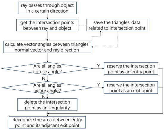
Figure 13.
Flowchart of improved ray-tracing method.
The structured meshes of the jagged target subdivided by using the ray-tracing method and improved ray-tracing method are shown in Figure 14, respectively. It can be seen from this figure that the meshes subdivided by using the conventional ray-tracing method are obviously erroneous while, by using the improved ray-tracing method, the jagged target is subdivided accurately. The accuracy of the meshes is improved obviously.
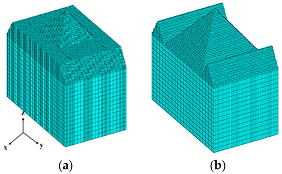
Figure 14.
Structured meshes of the jagged target. (a) Conventional ray-tracing method. (b) Improved ray-tracing method.
3. Results of Numerical Experiments
To demonstrate the effectiveness of the proposed mesh generation method, two numerical examples are used here for illustration. One is the Su-30 aircraft, representing an electrically large object, and the other is a complex antenna composed of multiple layers, thin lines, and small holes, representing typical fine structure models.
3.1. SU30 Aircraft
The scattering simulation of a large military target such as an aircraft, ship, and tank is important in radar detection. The Su-30 aircraft model shown in Figure 15 is a typical representative. The length of the aircraft is 21 m. The wingspan is 14 m and the height is 5 m. The whole structure is nonocclusive with two vents at the tail of the plane. Using Solidworks software to model the aircraft, the result is shown in Figure 16. It includes 5966 triangle elements totally.
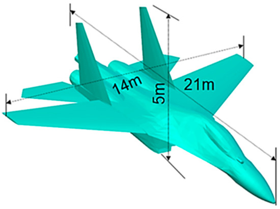
Figure 15.
The Su-30 aircraft model.
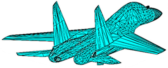
Figure 16.
Triangle elements of Su-30 aircraft mode.
The FDTD method is used to simulate the scattering field of the Su-30 aircraft. The simulation frequency ranges from 200 MHz to 500 MHz. Thus, the largest mesh size is set as 6 cm, corresponding to 1/10 of the minimum wavelength. By using the proposed mesh generation method, the structured meshes of the aircraft are obtained, as shown in Figure 17. The minimum mesh sizes in the X, Y, and Z direction are 3.742 cm, 3.738 cm, and 3.746 cm, respectively. The number of meshes in the X direction is 586, in the Y direction is 388, and in the Z direction is 148. The total number of meshes is 33,650,464. The generated mesh is shown in Figure 17. It can be seen from Figure 17 that the generated structured meshes fit the aircraft structure well. They maintain the geometric structural feature of the original model.
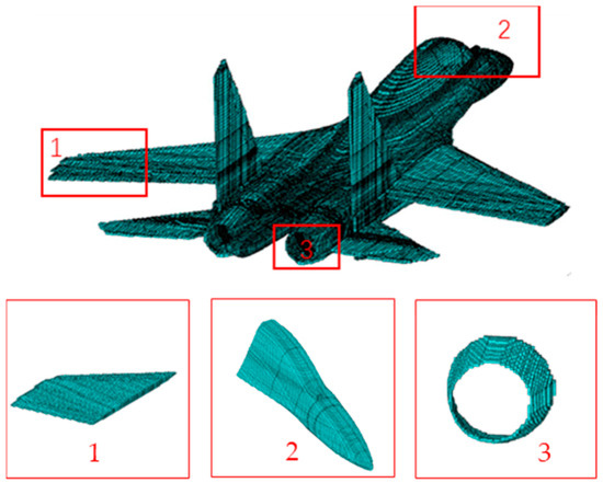
Figure 17.
The meshes of the aircraft generated by using proposed method.
However, if the conventional ray-tracing method is used to subdivide the aircraft, the result is shown in Figure 18. It can be seen from this figure that because of the singularity located at the wing, which has not been removed in the conventional ray-tracing method, the meshes exist with significant errors, resulting in poor fitting of the aircraft. The simulation time is shown in Table 1. The whole simulation is completed on a Windows PC using the Microsoft Visual Studio platform. It shows that the improved ray-tracing method occupied only a little more time than conventional ray tracing, but with much better accuracy.
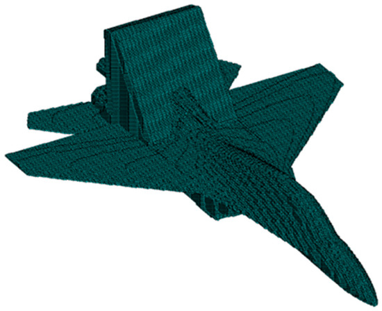
Figure 18.
The meshes of the aircraft generated by using conventional ray-tracing method.

Table 1.
Comparison of simulation time between conventional method and improved method.
To validate the accuracy of the meshes further, we calculate the radar cross section (RCS) of the Su-30 aircraft by using a parallel FDTD method based on the meshes in Figure 17 and compare the result with that of the CST software. In the FDTD simulation, an absorbing boundary with 10 cells is added to the computation domain. The domain between the absorbing boundary and the aircraft is also 10 cells, in which the incident wave is introduced. The size of these cells is 6 cm, corresponding to 1/10 of the minimum wavelength.
The simulated results are shown in Figure 19. It can be seen from the figure that, in the total frequency band from 200 MHz to 500 MHz, the backward RCS results calculated by using these two methods agree well with each other. In addition, the spatial distribution of the RCS in 250 MHz is also calculated. The results are shown in Figure 20. It can be seen from this figure that, in the whole space, from 0° to 360°, the two results match very well. These comparisons validate the high accuracy of the meshes indirectly.
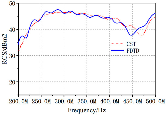
Figure 19.
RCS of Su-30 aircraft calculated by using CST software and FDTD method.
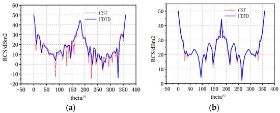
Figure 20.
Spatial distribution of RCS calculated by using CST software and FDTD method. (a) φ = 0 (250 MHz), (b) φ = 90 (250 MHz).
3.2. Bow-Tie Antenna
The antenna is an important device in wireless communication. With the expansion of application fields, modern antennas have a very complicated structure, including multiple layers, thin lines, small holes, etc. The bow-tie antenna shown in Figure 21 is a typical representative [12].
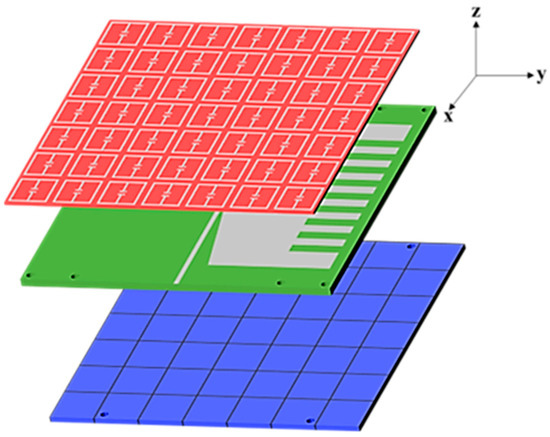
Figure 21.
Geometry of the bow-tie antenna.
This antenna is composed of a three-layer structure. The top layer is a metamaterial lens array that is used to improve the antenna gain. The middle layer is the main body of the bow-tie antenna. The bottom layer is an artificial magnetic conductor (AMC) reflector used to enhance the forward gain of the antenna. The thickness of these three dielectric plates, from top to bottom, is 0.813 mm, 2.4 mm, and 1.524 mm, respectively. The horizontal dimension of the whole structure is 420 mm × 420 mm. The detail dimensions of the antenna can be found in Ref. [12]. By using the mesh generation method, we obtain the structured meshes of the antenna, as shown in Figure 22. Due to it having a very fine metal strip, small holes, and fine slots on each layer, a uniform mesh is used in the X and Y direction. The whole XOY plane is subdivided by a 525 × 525 square mesh whose size is 0.8 mm × 0.8 mm. In the Z direction, the object is subdivided by non-uniform meshes. The number of meshes in this direction is 26. In the whole computational domain, the total number of meshes is 7,166,250.
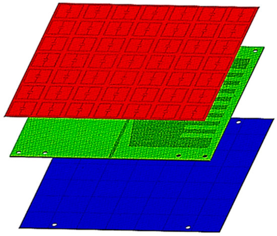
Figure 22.
The structured meshes of the antenna.
A detailed display of each layer is shown in Figure 23. It shows the subdivision details for small holes used to fix different boards, the curve for impedance matching, and the fine metal strip. From these figures, we can see that the generated structured meshes fit the antenna structure well, including the fine structures, such as small holes, thin strips, curves, etc.
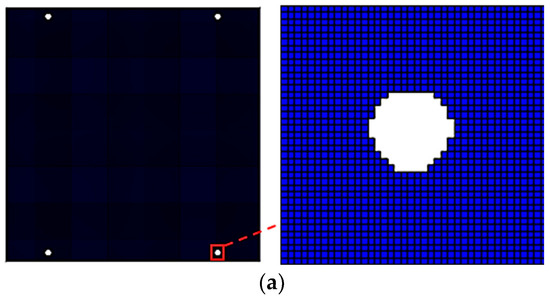
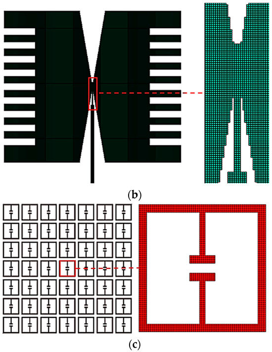
Figure 23.
Detailed display of each layer. (a) AMC reflector layer. (b) Bow-tie antenna layer. (c) Metamaterial lens layer.
To illustrate the accuracy of the generated meshes, we adopt a parallel FDTD program based on the meshes in Figure 22 to simulate the radiation pattern of the antenna, and compare the results with those of the CST software. The comparisons are shown in Figure 24. It shows the radiation patterns calculated at 460 MHz, 560 MHz, and 660 MHz, on the xz-plane and yz-plane, respectively. The radiation patterns show a high coincidence between the results of the FDTD method and CST software. The comparisons in Figure 24 also validate the high accuracy of the generated meshes.
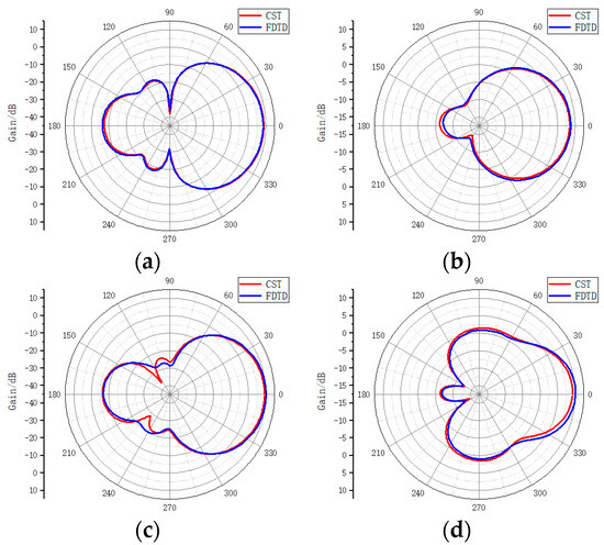
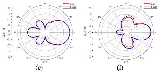
Figure 24.
Radiation patterns calculated by using CST software and FDTD method. (a) xz-plane at 460 MHz. (b) yz-plane at 460 MHz. (c) xz-plane at 560 MHz. (d) yz-plane at 560 MHz. (e) xz-plane at 660 MHz. (f) yz-plane at 660 MHz.
4. Conclusions
This paper presents a structured mesh generation method for FDTD simulation. The method takes an STL file as the input file and generates a non-uniform mesh according to the size of triangle elements. It uses an improved ray-tracing method to remove the singularity of the object and improves the mesh accuracy. To verify the effectiveness of this method, an Su-30 aircraft and a multi-layer bow-tie antenna are simulated. According to the comparison between the results of CST software and the FDTD algorithm, the mesh generation method has a high accuracy and can be applicable both for an electrically large model and fine structures.
Author Contributions
Conceptualization, J.W.; methodology, J.G.; software, J.G. and Z.X.; validation, C.M.; formal analysis, J.C.; writing, J.G. and J.C. All authors have read and agreed to the published version of the manuscript.
Funding
The authors declare that financial support was received for the research, authorship, and/or publication of this article. This work is supported by the Key Research and Development Program of China under Grants No. 2020YFA0709800, the National Natural Science Foundation of China (NNSFC) under Grants 62122061, and the Shaanxi Natural Science Basic Research Project of Shaanxi Science and Technology Office under Grants No. 2023-JC-QN-0673.
Data Availability Statement
Data are contained within the article.
Conflicts of Interest
The authors declare no conflicts of interest.
References
- Yee, K. Numerical solution of initial boundary value problems involving Maxwell’s equations in isotropic media. IEEE Trans. Antennas Propag. 1966, 14, 302–307. [Google Scholar]
- Sun, W.; Balanis, C.A.; Purchine, M.P.; Barber, G. Three-dimensional automatic FDTD mesh generation on a PC. In Proceedings of the IEEE Antennas and Propagation Society International Symposium, Ann Arbor, MI, USA, 28 June–2 July 1993; pp. 30–33. [Google Scholar]
- Gheonjian, A.; Jobava, R. Non-uniform conforming mesh generator for FDTD scheme in 3D cylindrical coordinate system. In Proceedings of the 5th International Seminar/Workshop on Direct and Inverse Problems of Electromagnetic and Acoustic Wave Theory (DIPED), Tbilisi, Georgia, 3–6 October 2000; pp. 41–44. [Google Scholar]
- Waldschmidt, G.; Taflove, A. Three-dimensional CAD-based mesh Generator for the Dey-Mittra conformal FDTD algorithm. IEEE Trans. Antennas Propag. 2004, 52, 1658–1664. [Google Scholar] [CrossRef]
- Okoniewski, M.; Okoniewska, E.; Stuchly, M.A. 3D sub-gridding algorithm for FDTD. In Proceedings of the IEEE Antennas and Propagation Society International Symposium, Newport Beach, CA, USA, 18–23 June 1995; pp. 232–235. [Google Scholar]
- Junkin, G.; Parron, J. A Robust 3D Mesh Generator for the Dey-Mittra Conformal FDTD Algorithm. In Proceedings of the Second European Conference on Antennas and Propagation, EuCAP 2007, Edinburgh, UK, 11–16 November 2007; pp. 1–6. [Google Scholar]
- Schuhmann, R.; Weiland, T. An improved implementation of nonorthogonal FDTD using triangular fillings. In Proceedings of the IEEE Antennas and Propagation Society International Symposium, Atlanta, GA, USA, 21–26 June 1998; pp. 600–603. [Google Scholar]
- Berens, M.K.; Flintoft, I.D.; Dawson, J.F. Structured Mesh Generation: Open-source automatic nonuniform mesh generation for FDTD simulation. IEEE Antennas Propagat. Mag. 2016, 58, 45–55. [Google Scholar] [CrossRef]
- Hong, L.; Kaufman, A.E. Fast projection-based ray-casting algorithm for rendering curvilinear volumes. IEEE Trans. Vis. Comput. Graph. 1999, 5, 322–332. [Google Scholar] [CrossRef][Green Version]
- Holland, R. Pitfalls of staircase meshing. In IEEE Transactions on Electromagnetic Compatibility; IEEE: New York, NY, USA, 1993; Volume 35, pp. 434–439. [Google Scholar]
- Chung, P.Y.; Wu, C.; Navarro, E.A.; Litva, J. A circular mesh scheme for the non-orthogonal finite difference time domain method. In Proceedings of the IEEE Antennas and Propagation Society International Symposium. 1995 Digest, Newport Beach, CA, USA, 18–23 June 1995; Volume 1, pp. 240–243. [Google Scholar]
- Li, Y.; Chen, J. Design of Miniaturized High Gain Bow-Tie Antenna. IEEE Trans. Antennas Propag. 2022, 70, 738–743. [Google Scholar] [CrossRef]


Disclaimer/Publisher’s Note: The statements, opinions and data contained in all publications are solely those of the individual author(s) and contributor(s) and not of MDPI and/or the editor(s). MDPI and/or the editor(s) disclaim responsibility for any injury to people or property resulting from any ideas, methods, instructions or products referred to in the content. |
© 2024 by the authors. Licensee MDPI, Basel, Switzerland. This article is an open access article distributed under the terms and conditions of the Creative Commons Attribution (CC BY) license (https://creativecommons.org/licenses/by/4.0/).