Heart Sound Signals Classification with Image Conversion Employed

Abstract

The number of patients with cardiovascular diseases worldwide is increasing rapidly, while medical resources are increasingly scarce. Heart sound classification, as the most direct means of discovering cardiovascular diseases, is attracting the attention of researchers around the world. Although great progress has been made in heart sound classification in recent years, most of them are based on traditional statistical feature methods and temporal dimension features. These traditional temporal dimension feature representation and classification methods cannot achieve good classification accuracy. This paper proposes a new partition attention module and Fusionghost module, and the entire network framework is named PANet. Without segmentation of the heart sound signal, the heart sound signal is converted into a bispectrum and input into the proposed framework for feature extraction and classification tasks. The network makes full use of multi-scale feature extraction and feature map fusion, improving the network feature extraction ability. This paper conducts a comprehensive study of the performance of different network parameters and different module numbers, and compares the performance with the most advanced algorithms currently available. Experiments have shown that for two classification problems (normal or abnormal), the classification accuracy rate on the 2016 PhysioNet/CinC Challenge database reached 97.89%, the sensitivity was 96.96%, and the specificity was 98.85%.

1. Introduction

Cardiovascular diseases pose a significant threat to global health, contributing to an increasing number of fatalities. Consequently, the importance of early prevention strategies for heart disease is of great significance [1]. Heart sound signals, which carry early pathological indicators of cardiovascular diseases, have been demonstrated to be effective in their early detection. Auscultation, a traditional method used by doctors to detect heart disease, involves the use of a stethoscope. This non-invasive, cost-effective technique requires only simple equipment, making it an ideal choice for cardiac examinations, particularly in smaller clinics with limited medical resources. However, the effectiveness of auscultation largely hinges on the clinical experience and skills of the doctor. While cardiologists achieve an accuracy rate of about 80% [2], primary care physicians typically reach only 20–40% [3]. Given these limitations, there is a pressing need for automated analysis and classification of heart sounds using computer-based methods.

Historically, heart sound signal processing has relied on traditional methods such as time-domain analysis and Mel Frequency Cepstral Coefficients (MFCC) [4]. These approaches, while foundational, often fail to capture the complex, non-linear characteristics of heart sounds, limiting their effectiveness in robust classification tasks. Furthermore, the sequential nature of heart sound signals poses additional challenges for traditional machine learning techniques and models, including Recurrent Neural Networks (RNN) [5], which, despite their aptitude for temporal data, struggle with capturing the intricate phase information and non-linear interactions present in heart sound signals.

To surmount these challenges, we pivot to bispectrum analysis for feature extraction, a method renowned for its proficiency in analyzing non-linear, non-Gaussian, and non-minimum phase stationary random signals. The bispectrum approach not only quantifies quadratic phase coupling and non-linear interactions but also maintains its effectiveness in noisy conditions, capturing the nuanced characteristics of heart sound signals with greater fidelity.

Our novel solution, the Partition Attention Network (PANet), leverages the bispectral analysis to transform heart sound signals into a two-dimensional image format, enabling the application of Convolutional Neural Networks (CNN) [6] for feature extraction and classification. This allows us to exploit the spatial processing strengths of CNNs, overcoming the limitations of traditional methods and RNNs in heart sound signal analysis. By integrating advanced bispectral feature representation with a sophisticated CNN architecture, our method marks a significant advancement in the automated analysis of heart sound signals, promising enhanced accuracy and efficiency in the classification tasks.

This work introduces a thoughtful advancement in heart sound signal classification by addressing the shortcomings of existing feature representations and learning models. Through the introduction of a novel feature representation and network architecture, we not only enhance the classification performance but also pave the way for more reliable automated heart sound analysis tools, offering a potent solution for the early detection and prevention of cardiovascular diseases.

The main contributions of this paper are as follows:

• In order to enable the network to learn the regional characteristics of the bispectrum, we propose a partition attention module based on the attention mechanism, which enables the network to automatically learn and assign different importance weights to different regions of the bispectrum.
• The deployment of the Partition Attention Module introduces a dynamic and effective method to recalibrate and emphasize the features within the bispectrum, significantly enhancing the model’s focus on critical regions.
• A novel features fusion module called FusionGhost is proposed to improve network feature extraction capability, and experiments show that it has better feature fusion and multi-dimensional extraction ability than Ghostnet module [7].

2. Related Work

This section provides a succinct overview of traditional machine learning methodologies, deep learning strategies, and techniques for converting time series data into images, specifically for heart sound classification.

2.1. Traditional Machine Learning Methods

The essence of heart sound classification involves extracting pivotal features from cardiac audio signals. A variety of studies [8,9,10,11,12] have implemented techniques encompassing statistical analysis, feature engineering, empirical wavelet transform (EWT) [13], and CNN for the extraction and segmentation of features in heart sound signals.

Post-extraction, the most distinctive features are identified for the classification process. Researches [8,11] have developed methodologies for selecting these features and incorporating them into classifiers for heart sound categorization. In [11], deep structured features created using a wavelet-based deep CNN were employed.

Subsequent to feature selection, the training and evaluation of models are performed. A range of machine learning models are evaluated to ascertain the most proficient classifier, as demonstrated in [9]. The paper [14] employed an ensemble learning approach that synergizes various features and classifiers to elevate the precision of automated heart sound classification. This method also achieved remarkable results in model evaluation, marked by elevated accuracy, sensitivity, specificity, and overall scores. In [15], wavelet analysis methods combined with a suite of deep learning models were used for heart sound classification, with experiments showing its superiority over previous techniques in two distinct datasets.

While traditional machine learning methods play a crucial role in heart sound classification, they are not without their drawbacks. These include intricate data preprocessing, the necessity to segment heart sound signals, and the potential for manually selected features to compromise robustness and generalizability. However, these methodologies still offer invaluable perspectives and act as foundational references in the domain of heart sound classification. Continuing to explore and enhance these methods remains imperative for the advancement of the field.

2.2. Rnn Methods

Heart sounds, inherent in their acoustic nature, exhibit a sequential pattern that is characteristic of time series. Recurrent Neural Networks, tailor-made for sequential data analysis, have shown remarkable efficacy in classifying such signals. This is evidenced in [16], where Bayesian Long Short-Term Memory (BLSTM [17]) networks have been successfully used to classify medical time series, such as heart sound recordings.

The research in [18] applied a windowed Discrete Fourier Transform (DFT) to each data sample, incorporating the variance and standard deviation of each window as distinctive features. This technique empowered the RNN to extract pivotal time series features, crucial for identifying anomalies in heart sounds.

In the study cited in [19], data framing ensures uniform sampling rates across all audio files, and down-sampling methods were implemented to lower the sound signal frequency, ensuring minimal performance degradation. Finally, an RNN was effectively used to classify these heart sound signals.

In [20], Logistic Regression-Hidden Semi-Markov Models (LRHSMM) were used for identifying heart states. After segmenting heartbeat recordings, the first 13 MFCCs were selected for a compact representation of the Phonocardiograms (PCG) [21] signal. Various RNN models were then applied for classification.

The study in [22] adopted an experimental method to establish effective feature subsets from both time-domain and frequency-domain features, with classification executed using LSTM. RNNs are instrumental in examining the long-term dependencies of time series attributes, facilitating the extraction of diverse features within the time and frequency domains of heart sound signals.

Although RNNs have demonstrated potential in classifying heart sounds, they are not without drawbacks. They particularly struggle with long data sequences due to the vanishing gradient issue, impeding their capability to discern long-term data dependencies. Moreover, RNNs necessitate extensive datasets and significant computational resources for effective training. In contrast, CNNs, especially in the context of spectrogram-based heart sound analysis, may provide a more efficient and robust approach for classifying heart sounds. This possibility merits further investigation in upcoming research.

2.3. CNN Methods

CNNs are leveraged for analyzing features from heart sound signals to identify useful patterns for classification.

In [23], an extensive array of 497 features from eight different domains was extracted and incorporated into the CNN framework. The authors of [24] recommended using advanced Mel-frequency cepstrum coefficient (MFCC) features alongside convolutional recurrent neural networks. This study also converted one-dimensional waveforms into two-dimensional time-frequency heat maps through MFCCs, where deep CNNs undertook both the feature extraction and classification tasks.

Another paper [25] focused on extracting Power Spectral Density (PSD) features, considering each PSD from a 5-second interval as a single-channel image, and used a convolutional architecture for processing. Meanwhile, [26] divided preprocessed PCGs into four distinct heart sound states based on a technique suggested in [27], followed by the extraction of 124 time-frequency features that were input into a CNN for analysis.

The authors of [28] presented an innovative CNN layer, featuring time-convolutional (tConv) units that replicate Finite Impulse Response (FIR) filters. Furthermore, [29] employed U-net for segmenting heart sounds, with CNNs conducting the classification. The study [30] demonstrates the use of Particle Swarm Optimization (PSO) for optimizing CNN hyper-parameters in environmental sound classification, indicating potential applications for enhancing heart sound analysis accuracy.

CNNs are beneficial in extracting heart sound signal features to some degree, facilitating the discovery of associations among diverse feature vectors. However, most examined methods primarily layer heart sound signal features like MFCC and Discrete Wavelet Transform (DWT) [31] for network input. This approach has its drawbacks as it does not maintain local feature consistency in the feature map. Consequently, this limits the convolutional neural network’s capability to effectively extract features pertinent for classification.

2.4. Methods for Converting Heart Sound Signals into Images

Several studies have devised techniques to convert time series data into image forms, leveraging computer vision for effective feature extraction and classification. Driven by deep learning’s breakthroughs in fields like computer vision and speech recognition, the researchers in [32] developed an innovative method to transform time series data into various image formats, including Gramian Angular Fields (GAF) and Markov Transition Fields (MTF), facilitating the application of computer vision methods in classification tasks. In this framework, GAF images are formed in a polar coordinate system and depicted as Gramian matrices, where each matrix element represents the cumulative trigonometric interactions across different time intervals. Meanwhile, MTF images illustrate the probabilities of first-order Markov transitions in one axis, while mapping time dependencies on another.

In research [33], a pioneering deep neural network was designed for recognizing human activities using data from multiple sensors. This design innovatively converts time series data from sensors into images, ensuring the preservation of key features necessary for accurate recognition of human activities.

While the methods of GAF and MTF have been effective in transforming time series data into images for classification, they have certain limitations. GAF, which represents images as a Gramian matrix using a polar coordinate system, may require substantial computational resources, especially for longer time series. Furthermore, GAF may lose some information during the transformation process. In contrast, MTF maps out first-order Markov transition probabilities and temporal dependencies across different dimensions. However, MTF only captures transitions between adjacent elements, potentially missing out on capturing transitions over larger time intervals.

2.5. Novelty and Comparison with Existing Techniques

In the field of heart sound signal processing, although traditional machine learning methods, RNN-based approaches, and existing CNN methods have made some progress, they still show significant limitations in handling complex signal characteristics, especially non-linear, non-Gaussian, and non-minimum phase stationary random signals. Addressing this challenge, this study proposes an innovative method for heart sound signal classification, which utilizes bispectral analysis to convert heart sound signals into images, followed by feature extraction and classification using CNN. Our method not only effectively quantifies quadratic phase coupling and non-linear interactions, but also, compared to traditional image encoding methods such as GAF and the MTF, bispectral imaging retains more original signal information, providing a richer feature learning foundation for CNN.

Furthermore, we introduced the Partition Attention Module (PA Module) and the FusionGhost Module, two innovative structures that significantly enhance the network’s ability to learn features from heart sound signals and optimize the automatic learning and fusion of features. The automatic emphasis on the most discriminative regions in the bispectral image by the PA Module further improves the accuracy and generalizability of the classification model. Meanwhile, the FusionGhost Module enhances feature expression by merging feature maps of different scales, significantly improving classification performance.

Table 1. Comparative analysis of heart sound signal processing methods.

Feature/Method	Traditional ML	RNN Methods	CNN Methods	Other Image Conversion Methods	Our Method (Bispectral Imaging + CNN)
Feature Extraction	Manual	Sequential	Raw/Simple	Limited	Bispectral for non-linear features
Signal Conversion	None	None	Limited	GAF, MTF	Bispectral retains more information
Non-linear Feature Handling	Limited	Limited	Limited	Limited	Efficient
Complex Signal Processing	Low	Moderate	Moderate	Moderate	High
Noise Robustness	Limited	Limited	Limited	Limited	Significantly enhanced
Automatic Feature Learning	None	Yes	Yes	Limited	Strong
Attention to Key Areas	None	None	None	None	PA Module
Feature Fusion Strategy	Stacking	Temporal Fusion	Multi-layer Fusion	Simple	FusionGhost improves fusion

summarizes the comparison between our method and existing technologies, highlighting the innovations and advantages of this research:

Through this comparison, it is evident that our research demonstrates significant advantages in capturing non-linear features, signal conversion efficiency, classification performance, as well as handling complex signals and robustness to noise compared to traditional methods and existing technologies. These innovations not only advance the development of heart sound signal processing technology but also provide an efficient and accurate technical solution for the early diagnosis and monitoring of cardiovascular diseases.

In conclusion, this study introduces a novel approach in heart sound signal classification by integrating bispectral imaging with advanced CNN architectures. The subsequent sections will detail the specific methodologies employed, further illustrating the effectiveness and efficiency of our proposed solution in addressing the challenges of heart sound signal analysis.

3. Methodology

Our heart sound classification approach, as depicted in Figure 1, begins with the preprocessing of the initial heart sound signals to eliminate noise. This is followed by the transformation of these preprocessed signals into bispectra. The bispectra, serving as inputs, are then trained through PANet to yield a classification model. During the testing phase, test samples undergo the same preprocessing and bispectrum generation steps, and are subsequently inputted into the trained network model to obtain classification results. This method capitalizes on the strengths of CNNs in feature extraction and classification, and effectively carries out heart sound classification. Moreover, the use of bispectra offers its own advantages. It transforms one-dimensional heart sound signals into two-dimensional images, facilitating subsequent feature extraction and classification. In the following sections, we will delve into the specifics of each step and their methodologies. This comprehensive approach not only harnesses the power of CNNs but also leverages the unique benefits of bispectra, providing an effective and efficient solution for heart sound classification.

3.1. Signal Preprocessing

In the signal preprocessing stage of our heart sound classification method, we apply a fifth-order Butterworth band-pass filter [34] with a passband of 25–400 Hz. This filter is instrumental in eliminating low-frequency artifacts, baseline drift, and high-frequency interference from the originally acquired heart sound signals. The Butterworth filter is chosen for its flat frequency response in the passband and sharp rolloff, defined by the transfer function:

$$H\left(f\right)=\frac{1}{\sqrt{1+{\left(\frac{f}{f_c}\right)}^{2n}}}$$

(1)

where f is the frequency, $f_c$ is the cutoff frequency, and n is the order of the filter. In our application, the passband is specifically set to 25–400 Hz to focus on the frequency components relevant to heart sound signals.

Additionally, the raw heart sound signals are normalized [35] to a range between −1 and 1 to ensure consistency in signal amplitude across all samples. This normalization is crucial for facilitating a fair comparison and analysis of the signals, regardless of their original amplitude levels. The normalization formula is as follows:

$$x_{norm}=\frac{x-\min \left(x\right)}{\max \left(x\right)-\min \left(x\right)}\times 2-1$$

(2)

where x represents the original signal. This process scales the amplitude of the signals, ensuring uniformity across the dataset.

The combination of Butterworth filtering and normalization significantly enhances the clarity and quality of the heart sound signals, as can be seen in the improved signal profiles shown in Figure 2. The preprocessing step ensures that the heart sound signals are streamlined and standardized, providing a clean baseline for the accurate detection and classification of cardiac events. The filtered signals exhibit a reduction in background noise and artifacts, while the normalization process ensures a consistent signal amplitude across all recordings, which is crucial for the subsequent automated analysis.

3.2. Bispectrum Feature Representation

In our heart sound signal classification methodology, the generation of the bispectrum is a crucial step that transforms the original one-dimensional heart sound signal into a two-dimensional image rich in frequency and phase information. This transformation begins with preprocessing the heart sound signals to reduce noise and enhance signal quality. Subsequently, we employ the Fourier Transform to decompose the processed signal into its frequency components, capturing the signal’s fundamental spectral information. Following this, we apply the Short-Time Fourier Transform (STFT) to analyze these frequency components over localized time intervals, obtaining the signal’s dynamic time-frequency information. Finally, we compute the correlations between these frequency components to derive the bispectrum. The bispectrum quantitatively captures the quadratic phase coupling of frequency components in the signal, encoding the heart sound signal into a comprehensive two-dimensional bispectrum image. This image encompasses not only amplitude information but also phase information, providing a robust feature set for further analysis using CNNs.

3.2.1. Fourier Transform

The Fourier Transform plays a pivotal role in audio signal processing. It has the ability to decompose complex audio signals into a series of simple sine and cosine waves. The frequency, amplitude, and phase of these waves can be used to fully reconstruct the original signal. This capability makes the Fourier Transform a fundamental tool for audio signal analysis, as it can reveal the spectral characteristics of the audio signal, i.e., the intensity of each frequency component in the signal.

The mathematical definition of the Fourier Transform includes both continuous and discrete forms. The formula for the continuous Fourier Transform is:

$$F\left(\omega \right)={\int }_{-\infty }^{+\infty }f\left(t\right)e^{-i\omega t}dt$$

(3)

where $F\left(\omega \right)$ is the function after the Fourier Transform, $f\left(t\right)$ is the original function, $\omega$ is the frequency, and t is the time. The formula for the Discrete Fourier Transform (DFT) is:

$$X\left(k\right)=\sum _{n=0}^{N-I}x\left(n\right)e^{-i2\pi kn/N}$$

(4)

where $x\left(k\right)$ is the result of the Discrete Fourier Transform, $x\left(n\right)$ is the discrete input signal, k is the discrete frequency, and N is the length of the signal. These formulas describe how to transform a signal from the time domain to the frequency domain.

However, a major limitation of the Fourier Transform is that it can only provide global frequency information of the signal, and cannot provide time-frequency information of the signal. In other words, the Fourier Transform cannot tell us when a certain frequency component appears in the signal. To solve this problem, the Short-Time Fourier Transform (STFT) was proposed. The STFT applies the Fourier Transform to different parts of the signal, providing time-frequency information of the signal.

3.2.2. STFT

Short Time Fourier Transform, as shown in Equation (5), is a time-frequency analysis algorithm commonly used to analyze non-stationary signals. It divides the signal into many small time intervals, considers that the signal tends to be stable in each time interval, and carries out Fourier transform in each time interval in order to determine the frequency distribution of each time period.

$$X(n,\omega )=\sum _{m=-\infty }^{+\infty }x\left(m\right)\omega (n-m)e^{-j\omega m}$$

(5)

3.2.3. Bispectrum

The Bispectrum, a higher-order spectral analysis technique, provides a comprehensive representation of a signal by quantifying the coupling relationship between its oscillatory components. It extracts nonlinear coupling features and generates a complete coupling feature map across different frequencies.

In more detail, the Bispectrum is a third-order spectral analysis method that captures the phase coupling information which is typically missed by power spectrum methods. Mathematically, for a discrete signal $X\left(f\right)$, its bispectrum $Bis(f_1,f_2)$ is defined as

$$Bis(f_1,f_2)=\underset{T\to \infty }{lim}\left(\frac{1}{T}\right)E\left[X(f_1+f_2)X^{*}\left(f_1\right)X^{*}\left(f_2\right)\right]$$

(6)

where E denotes the expectation, * denotes the complex conjugate, and $f_1, f_2$ are the frequencies.

This formula illustrates how the bispectrum captures phase coupling information in the signal: if components at frequencies $f_1$ and $f_2$ exist in the signal and their phases are coupled, then the value of the bispectrum at $(f_1,f_2)$ will be non-zero. The bispectrum captures phase coupling in signals, mapping frequency domain characteristics and phase coupling characteristics onto a two-dimensional image via Fourier transform and second-order moment. This mapping is bijective, allowing signal recovery from the bispectrum. However, as it captures only second-order statistical characteristics, higher-order nonlinearities or phase couplings may not be captured.

In summary, the bispectrum is a potent tool for encoding heart sound signals into images, preserving feature relationships and facilitating local feature extraction using CNNs. Each pixel in the image represents a feature, and spatial relationships between pixels represent feature relationships, providing more information for effective feature extraction and classification.

3.3. Classification Network Framework

In this section, we introduce a novel network architecture named Partition Attention Network (PANet), which is based on CNN. This innovative architecture is designed to enhance the efficiency and accuracy of heart sound classification tasks. The PANet is composed of several key components, each playing a crucial role in the network’s performance. These components include the Network Structure, the Partition Attention Module, and the FusionGhost Module. As we delve deeper into this section, we will provide a detailed description of each component and explain how they collectively contribute to the superior performance of the PANet.

Network Structure

Figure 3 illustrates the overall network structure of the proposed PANet and the input and output sizes of each module are shown in

Table 2. Network structure.

Layers	Input Size	Output Size	Parms	FLOPs
PA module	256 × 256 × 1	128 × 128 × 4	2,097,796	4,195,196
Conv1	128 × 128 × 4	128 × 128 × 64	320	7,340,032
Inception1	128 × 128 × 64	128 × 128 × 64	38,912	151,011,944
Concat & Pooling	128 × 128 × 64	64 × 64 × 128	0	2,097,152
Inception2	64 × 64 × 128	64 × 64 × 128	51,200	209,715,200
Conv2	64 × 64 × 128	32 × 32 × 128	295,168	301,989,888
Inception3	32 × 32 × 256	32 × 32 × 256	205,312	244,366,784
Conv3	32 × 32 × 256	16 × 16 × 256	590,080	150,994,944
FusionGhost Module1	16 × 16 × 256	8 × 8 × 128	147,456	9,437,184
FusionGhost Module2	8 × 8 × 128	4 × 4 × 64	36,864	589,824
Classification Layer	4 × 4 × 64	2	2050	4094

. The input of the network is bispectrum. PA module make use of the attention mechanism to assign different importance weights to different areas of the bispectrum, so that the network can pay more attention to the parts that need attention. After that, a larger receptive field can be obtained through the stacking of multi-layer convolution.

The integration of different scale features is realized through the Inception structure [36]. It is known for its efficient utilization of computing resources within the network. It achieves this by incorporating multiple kernel sizes in each layer of the network, allowing it to capture complex features from both global and local perspectives effectively. In our PANet, we have adapted this architecture to enhance its feature extraction capability specifically for heart sound signals represented as bispectrums. This adaptation ensures that intricate patterns embedded within different frequency bands are captured comprehensively.

In the context of our network structure, the Inception modules (Inception1, Inception2, and Inception3) are used to integrate different scale features. As shown in Table 2, each Inception module takes an input with a certain size and outputs a feature map of the same size, but with more channels. This means that the Inception modules are able to extract more complex features without changing the spatial dimensions of the feature maps. This is particularly useful for tasks like heart sound classification, where the spatial structure of the input (in this case, the bispectrum) contains important information.

In parallel to the advanced Inception structures, our PANet incorporates a series of convolutional layers, namely conv1, conv2, and conv3, each serving a distinct purpose in the feature extraction process. The conv1 layer, receiving the attention-weighted bispectrum from the PA module, initiates the feature extraction with multiple filters, expanding the depth of the feature maps while preserving spatial resolution. This is followed by a novel concat and pooling operation, where the outputs of conv1 and Inception1 are concatenated along the channel dimension, effectively amalgamating their feature representations. A subsequent pooling step not only compresses the spatial dimensions but also amplifies the depth of the features, setting the stage for deeper feature integration in the subsequent layers. As the signal progresses through conv2, the network performs a pivotal operation: The feature maps are scaled up by a factor of two in conv2, capturing finer details vital for precise heart sound classification. After this, a Channel Shuffle is executed to mix these channels. This ensures a more holistic learning of features, as it encourages different filters to share information, leading to a more generalized and robust feature representation. The shuffle not only prevents over-specialization of filters on certain feature types but also aids in maintaining effective feature diversity. Consequently, this elevates the network’s ability to discern subtle patterns within the heart sound signals, crucial for accurate classification. After further refinement through Inception2, the signal is propelled through conv3, which acts as a bridge to the sophisticated FusionGhost modules, seamlessly transitioning from dense feature maps to more abstract representations, priming the network for the final classification task.

While convoluting the feature map, the FusionGhost module performs linear transformation and stitching with the convolution results, not only improving convolution efficiency but also maintaining consistency of features. Finally, the full connection layer aggregates all features and obtains the probability of classification.

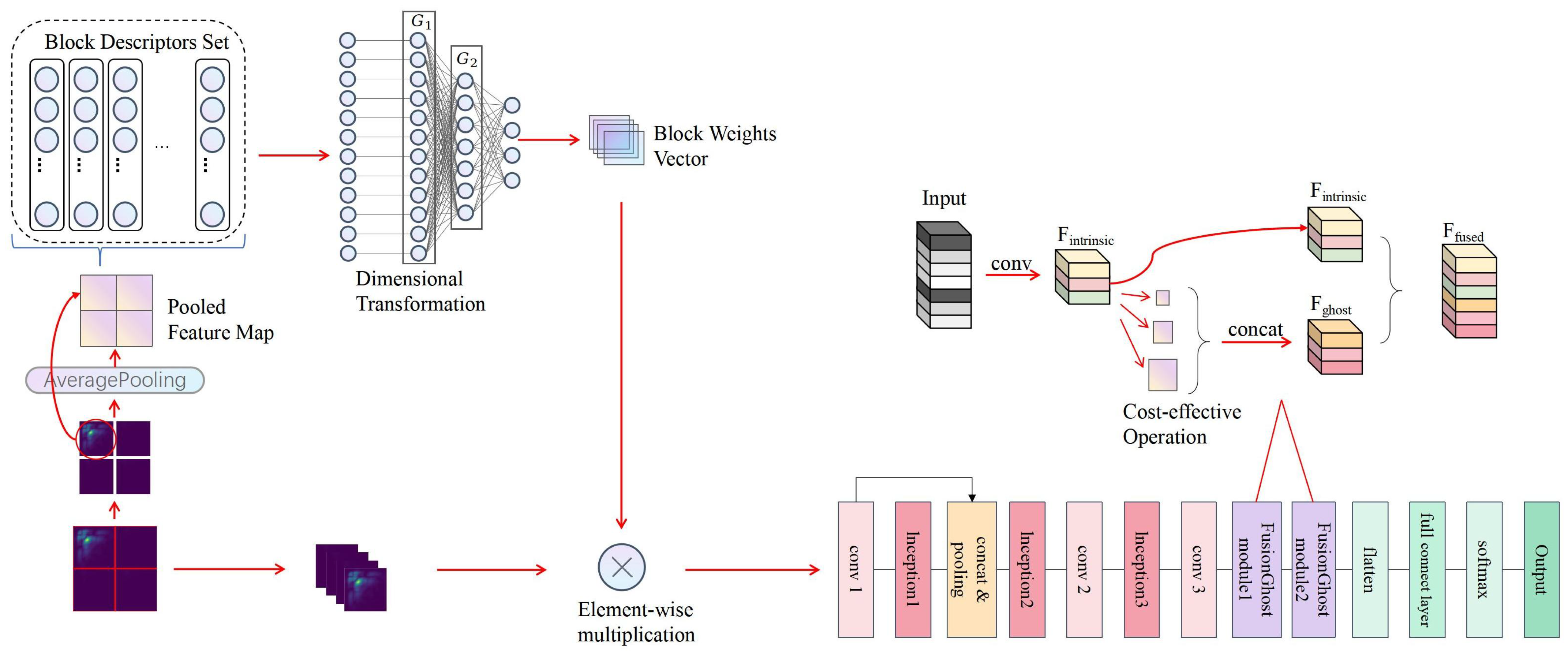
3.4. Partition Attention Module

Our heart sound signal classification framework features the innovative Partition Attention Network (PANet), a key development that significantly elevates the model’s proficiency in isolating and analyzing critical features of heart sound signals. Central to this enhancement is the Partition Attention Module, a sophisticated mechanism designed to meticulously partition the input feature map, thereby facilitating a more granular analysis of the acoustic signals. 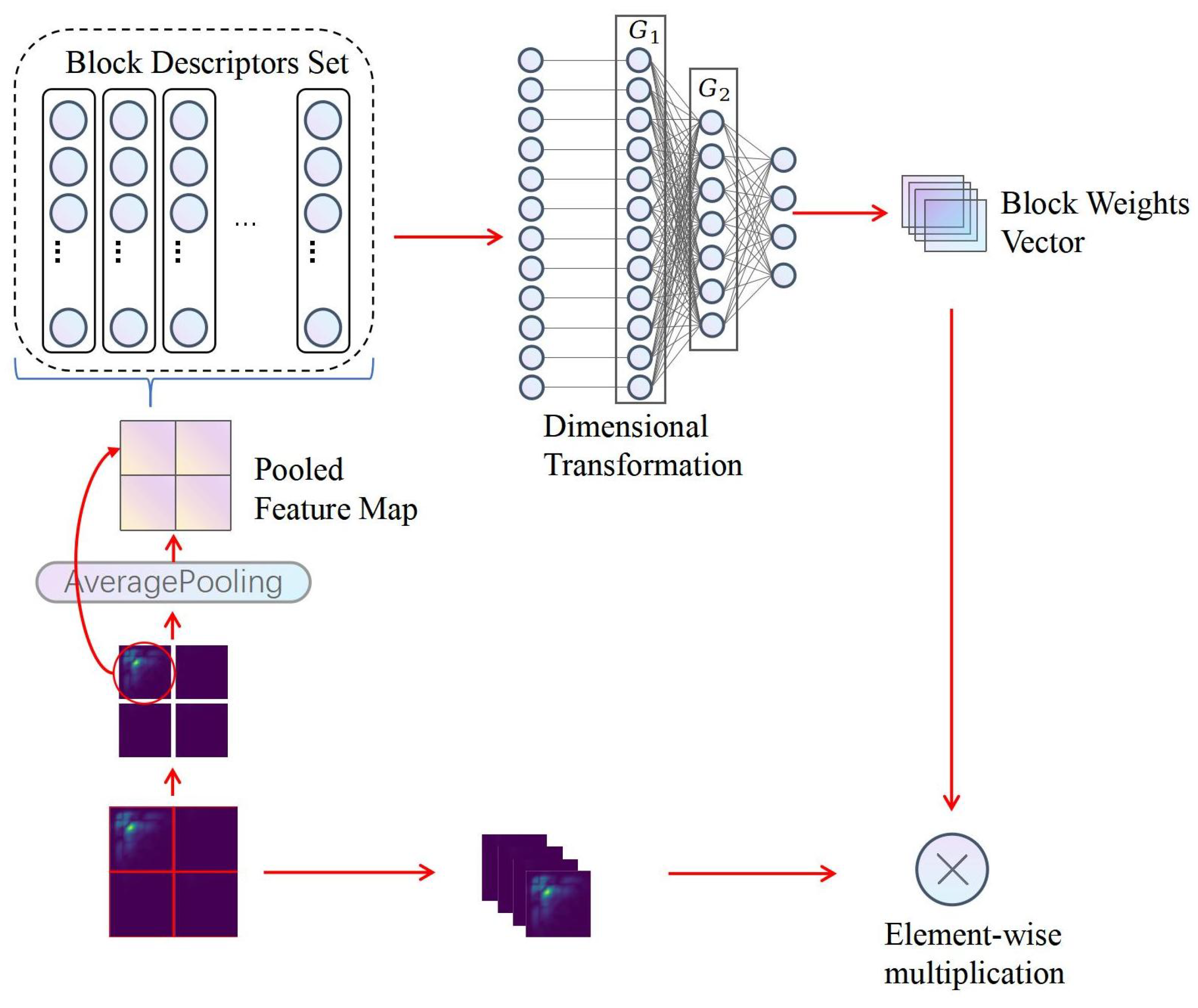Figure 4 provides a detailed visual representation of the nuanced operations within the Partition Attention Module, beginning with a bispectrum as the initial input. This bispectrum is processed through a Partition Mechanism, segmenting the signal into distinct blocks, which are subsequently streamlined via an Average Pooling layer into a pooled feature map.This streamlined process paves the way for Global Feature Vector Extraction, where a Block Descriptors Set is formulated, encapsulating the essential traits of the signal. The journey of data transformation continues with a Dimensional Transformation, preparing the data for the subsequent stages of processing. A critical phase follows, where a Weight Allocation layer assigns a vector of block weights, ingeniously designed to magnify the significant features within the heart sound signals through an element-wise multiplication with the initial blocks. This methodical enhancement of pivotal features underscores the advanced capability of PANet in accentuating crucial patterns within the heart sound signals, thereby underlining the framework’s enhanced effectiveness in the precise classification of these signals.

Partition Mechanism: The initial step involves uniformly dividing the input two-dimensional feature map (e.g., 256 × 256 × 1) into B equivalent blocks, where $B=4$ serves as a typical example, with each block having dimensions of 128 × 128. This segmentation not only divides the feature map physically but also logically treats each block as an individual channel, enabling detailed local feature extraction.

Average Pooling Layer: Each block is subjected to an average pooling operation to reduce its dimensionality. Average pooling computes the mean of the elements within a specified neighborhood, effectively condensing the information into a more compact representation. For a block of size $n\times n$, the average pooling operation with a pooling size of $k\times k$ is defined as:

$$P(i,j)=\frac{1}{k^2}\sum _{s=0}^{k-1}\sum _{t=0}^{k-1}I(i+s,j+t)$$

(7)

where $P(i,j)$ is the pooled value, $I(i,j)$ is the original value at the $(i,j)$th position in the block, and the summation is carried out over the $k\times k$ neighborhood.

Global Feature Vector Extraction: After average pooling, each block is transformed into a global feature vector. This vectorization step converts the pooled $n/k\times n/k$ block into a one-dimensional array of length ${(n/k)}^2$, capturing the essence of the block’s features. The transformation is represented by:

$$\mathbf{v}=\mathrm{vec}\left(P\right)$$

(8)

where $\mathbf{v}$ is the global feature vector and $\mathrm{vec}\left(P\right)$ denotes the vectorization of the pooled block P.

Block Descriptors Set: The global feature vectors from all blocks are concatenated to form the feature vector set $\mathbf{V}$, represented as a matrix: $\mathbf{V}=\left(\begin{array}{cccc}{\mathbf{v}}_1& {\mathbf{v}}_2& \dots & {\mathbf{v}}_B\end{array}\right)$, where each ${\mathbf{v}}_i$ is the vectorized representation of block i.

Dimensional Transformation: To process these feature vectors and extract pivotal information for the classification task, two fully connected layers, represented as linear transformation layers, $G_1$ and $G_2$, are employed. $G_1$ reduces the dimensions of the feature vectors in $\mathbf{V}$, aiming to simplify computations and highlight key features. The dimensions of $G_1$ are defined as ${\mathbb{R}}^{\frac{N}{r}\times N}$, where r is the reduction ratio. Subsequently, $G_2$ maps the output of $G_1$ to the final number of blocks B, with dimensions ${\mathbb{R}}^{B\times \frac{N}{r}}$.

Weight Allocation Layer: The linear transformations provided by $G_1$ and $G_2$ generate a set of weights $\omega$ for each block. These weights are computed by passing the feature vector set $\mathbf{V}$ through $G_1$ for dimension reduction, followed by an application of the ReLU function [37] for non-linear activation, and finally through $G_2$ for mapping to the weight space corresponding to the number of blocks B. This process is mathematically represented as:

$$\omega =\mathrm{ReLU}\left(G_2\left(G_1\left(\mathbf{V}\right)\right)\right)$$

(9)

where the ReLU function introduces non-linearity, aiding the model in learning complex patterns of weight distribution. The weight vector $\omega$ represents the importance of each block for the classification task, allowing the model to focus more on blocks containing significant information.

These weights are then used to reweight the feature map, producing the output of the PA module. Each block’s original features $u_n$ are multiplied by their corresponding weights ${\omega }_n$, yielding reweighted features which emphasize the more informative parts of the input. The operation for obtaining the final weighted feature map is given by:

$${\tilde{P}}_n=u_n·{\omega }_n$$

(10)

where ${\tilde{P}}_n$ represents the reweighted feature of the n-th block. This reweighting process ensures that the network prioritizes blocks with essential information, significantly improving the overall performance of the model.

3.5. FusionGhost Module

In our heart sound signal classification framework, the FusionGhost module plays a crucial role in enhancing the depth and breadth of feature extraction while optimizing computational efficiency and strategically fusing features. After the heart sound signals have been processed through a series of convolutional layers, enriched by the Inception modules, and integrated via a concat and pooling operation. Following these initial processes, the FusionGhost module takes action. As Figure 5 illustrates, this module begins by passing the input through a convolutional layer, creating a set of intrinsic feature maps, denoted as $F_{intrinsic}$. In a parallel process, these $F_{intrinsic}$ feature maps are subjected to a series of cost-effective operations aimed at generating additional feature maps efficiently. The outputs of these operations are then concatenated, and it is this concatenated outcome that is identified as $F_{ghost}$. These ghost feature maps, crafted to enrich the signal representation without a hefty computational cost, are fused with the intrinsic feature maps. The resulting concatenation, $F_{fused}$, is the culminating output comprising the fused feature maps that incorporate comprehensive information from both intrinsic and ghost operations. The strategic placement of the FusionGhost module ensures that the network not only leverages pivotal information from the heart sound signals but also synthesizes and refines this information in a computationally savvy manner, significantly enhancing classification accuracy.

3.5.1. Primary Convolution

Within the FusionGhost module, the primary convolution layer ($Con{v}_{primary}$) is defined as the first convolution operation processing the input feature map $X\in {\mathbb{R}}^{H\times W\times C_{in}}$, where H, W, and $C_{in}$ respectively denote the height, width, and the number of channels of the input feature map. The purpose of this convolution layer is to generate a set of intrinsic feature maps $F_{intrinsic}$, laying the groundwork for subsequent feature map expansion. The operation of the primary convolution layer can be expressed as

$$F_{intrinsic}=Con{v}_{primary}(X;{\theta }_{primary})$$

(11)

where ${\theta }_{primary}$ represents the parameters of the primary convolution layer, including the weights and bias of the convolution kernels. $F_{intrinsic}\in {\mathbb{R}}^{H^{\prime }\times W^{\prime }\times C_m}$, with $C_m$ being the number of channels in the intrinsic feature maps, and $H^{\prime }$ and $W^{\prime }$ being the height and width of the feature maps after convolution, which depend on the size of the convolution kernel, padding, and stride.

The computational cost of the primary convolution layer is primarily determined by its convolution operation, which can be estimated by the following formula:

$${\mathrm{Cos}\mathrm{t}}_{primary}=H^{\prime }\times W^{\prime }\times C_{in}\times C_m\times K^2$$

(12)

where K is the size of the convolution kernel. To reduce computational cost, $C_m$ is typically chosen to be less than $C_{in}$, and K is selected to be as small as possible. The principle of choosing $C_m$ is to minimize the computational cost while ensuring sufficient feature extraction capability. Ideally, the value of $C_m$.

3.5.2. Cost-Effective Operations and Feature Fusion Strategy

The FusionGhost module introduces cost-effective linear operations through the $\Phi$ function, aimed at expanding the network’s feature representation capacity with minimal computational resource consumption. This function applies a series of operations to the intrinsic feature maps $F_{intrinsic}$ produced by the primary convolution layer, generating the so-called ghost feature maps $F_{ghost}$, mathematically expressed as

$$F_{ghost}=\Phi (F_{intrinsic};{\theta }_{\Phi })$$

(13)

where ${\theta }_{\Phi }$ represents the parameters involved in the $\Phi$ function, and $F_{ghost}$ are the ghost feature maps obtained through these cost-effective operations. These operations include the use of small-scale convolution kernels and linear activations, effectively expanding the model’s width and capacity.

In processing heart sound spectrograms, the $\Phi$ operation’s multi-scale convolution kernels significantly enhance the model’s ability to comprehend input data, especially crucial in handling the complexity of heart sound signals. To maintain the consistency of output feature map dimensions after applying convolution kernels of different scales, it is necessary to adjust the padding of each convolution operation appropriately, calculated as $⌊\frac{k - 1}{2}⌋$, ensuring the dimensions of the output feature map consistent with the input, providing a solid foundation for subsequent feature fusion.

To generate the additional $n-m$ ghost feature maps, an equal distribution strategy is chosen, where each scale of the $\Phi$ operation is responsible for generating an equal number of ghost feature maps. Therefore, each scale of convolution kernels ($1\times 1$, $3\times 3$, $5\times 5$) will generate $\frac{n-m}{3}$ ghost feature maps. These feature maps are then directly concatenated with the intrinsic feature maps $F_{intrinsic}$, forming the final output feature map set $F_{fused}=\mathrm{Concat}(F_{intrinsic},F_{ghost})$. Through this design, the FusionGhost module enriches the model’s feature representation while controlling the overall computational cost, making it suitable for environments with limited computational resources.

By combining cheap operations with a feature fusion strategy, not only is the section made more concise, but it also focuses on the core functionality and implementation method of the module, making the overall description more compact and understandable.

3.5.3. Computational Complexity

The theoretical speed-up ratio ($r_s$) of employing the FusionGhost module over traditional convolution is calculated by comparing the computational complexities of both operations. According to the design principles of the FusionGhost module, the speed-up ratio can be expressed as

$$r_s=\frac{n·h^{\prime }·w^{\prime }·c·k·k}{\frac{n}{s}·h^{\prime }·w^{\prime }·c·k·k+(s-1)·\frac{n}{s}·h^{\prime }·w^{\prime }·d·d}$$

(14)

where $d\times d$ is similar in magnitude to $k\times k$, and s is much smaller than c. This equation indicates that the FusionGhost module not only minimizes computational costs but also accelerates model operation, making it particularly beneficial for processing extensive datasets typical in heart sound signal classification tasks.

Similarly, the compression ratio can be calculated as

$$r_c=\frac{n·c·k·k}{\frac{n}{s}·c·k·k+(s-1)·\frac{n}{s}·d·d}\approx \frac{s·c}{s+c-1}\approx s,$$

(15)

which equals the speed-up ratio achieved by the FusionGhost module. This analysis underscores the module’s effectiveness in reducing memory usage and computational costs, thus facilitating efficient network operation even in resource-constrained environments.

By integrating the FusionGhost module, networks not only enjoy reduced computational complexity and enhanced operational speed but also maintain high accuracy in feature representation and classification tasks, especially in analyzing complex heart sound spectrograms.

3.6. Computation Analysis

The parameters of the PA module mainly come from the fully connected layer. The number of neurons in G1 is 64 × 64 × 4, in G2 is 128, and in the final output layer is 4. Therefore, the number of parameters can be calculated by 64 × 64 × 4 × 128 + 128 + 128 × 4 + 4, resulting in a total of 2,097,796 parameters for the PA module. The computational load of the PA module primarily originates from the Average Pooling and the fully connected layer. The computational load of Average Pooling is: 128 × 128 × 4, and the fully connected layer is: 64 × 64 × 4 × 128 + (64 × 64 × 4 − 1) × 128 + 128 × 4 + 127 × 4. Thus, the total computational load of the PA module is the sum of these two parts, amounting to 4,195,196.

Conv1’s convolutional kernel size is 1 × 1 × 64, with a stride of 2. Therefore, the number of parameters for Conv1 can be calculated as 1 × 1 × 4 × 64 + 64, and its computational load is 128 × 128 × 64 × (4 + 4 − 1). Thus, Conv1 has 320 parameters and a computational load of 7,340,032.

Inception1 module’s parameters and computational load are derived from four branches: one with a 1 × 1 convolution, one with a 1 × 1 and a 3 × 3 convolution, one with a 1 × 1 and a 5 × 5 convolution, and one with a 3 × 3 max pooling and a 1 × 1 convolution. With input and output sizes both at (128, 128, 64), the total parameter count for Inception1 sums up to 38,912, calculated from the individual branches’ parameters (1024 + 10,240 + 26,624 + 1024), and the total computational load reaches 151,011,944, derived from the computational loads of each branch (2,097,152 + 39,845,888 + 106,954,752 + 2,097,152).

For Concat+Pooling, there are no parameters involved, and the computational load primarily stems from the pooling operation. This operation utilizes average pooling, with an input dimension of (128, 128, 128) and an output dimension of (64, 64, 128), using a pooling size of (2, 2) and a stride of 2. Consequently, the computational load is calculated to be 2,097,152, following the formula 64 × 64 × 128 × 4.

Inception2 module’s parameters and computational load are derived from four branches: one with a 1 × 1 convolution, one with a 1 × 1 and a 3 × 3 convolution, one with a 1 × 1 and a 5 × 5 convolution, and one with a 3 × 3 max pooling and a 1 × 1 convolution. Inception2 operates with an input and output size of (64, 64, 128). The total parameters for Inception2 are derived from the sum of its branches’ parameters, amounting to 51,200. Similarly, the computational load of Inception2 is the sum of its branches’ computational load, totaling 209, 715, 200.

Conv2 processes inputs of size (64, 64, 128) and outputs of (32, 32, 128) using 3 × 3 convolutions with a stride of 2. To enhance the model’s feature extraction capabilities, we employed two instances of Conv2. Each Conv2 has a parameter count of (3 × 3 × 128 + 1) × 128 and a computational load of 32 × 32 × 128 × (3 × 3 × 128). Thus, with two Conv2 layers, the total parameters amount to 295,168, and the combined computational effort is 301,989,888.

Inception3 module’s parameters and computational load are derived from four branches: one with a 1 × 1 convolution, one with a 1 × 1 and a 3 × 3 convolution, one with a 1 × 1 and a 5 × 5 convolution, and one with a 3 × 3 max pooling and a 1 × 1 convolution. Inception3 operates with input and output dimensions of (32, 32, 256). The total parameters for Inception3, aggregated from its individual branches, amount to 205,312, calculated as 16,384 × 4 + 36,864 + 102,400. Likewise, its computational load, summed from the contributions of each branch, totals 244,366,784, with a calculation breakdown of 16,777,216 × 4 × 47,185,920 × 131,072,000.

Conv3 with an input size of (32, 32, 256) and reduces the output to (16, 16, 256) through 3 × 3 convolutions with a stride of 2. The total parameters for Conv3 are calculated as 3 × 3 × 256 + 1) × 256, which equals 590,080. The computational load for Conv3 is determined by the formula 16 × 16 × 256 × 3 × 3 × 256), resulting in 150,994,944 operations.

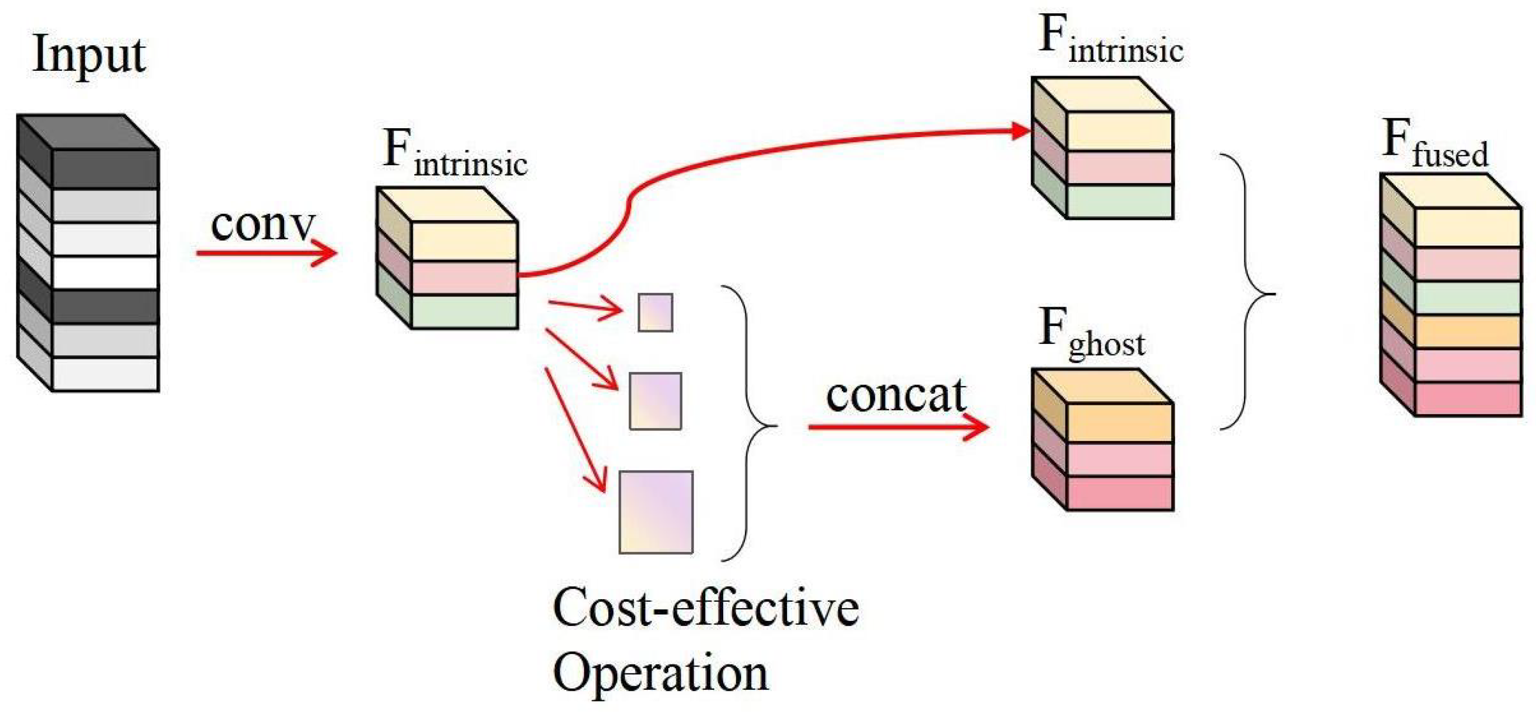
FusionGhost Module1 has an input dimension of (16, 16, 256) and produces an output of (8, 8, 128). It involves 147,456 parameters, calculated from 3 × 3 × 256 × 64, and its computational operations amount to 9,437,184, determined by 3 × 3 × 256 × 8 × 8 × 64.

FusionGhost Module2 takes an input of (8, 8, 128) and yields an output dimension of (4, 4, 64). This module requires 36,864 parameters, computed as 3 × 3 × 128 × 32, and its total computational operations are 589,824, derived from 3 × 3 × 128 × 4 × 4 × 32.

The Classification Layer includes a Flatten operation and a fully connected layer. The input size is (4, 4, 64), and it is flattened into 4 × 4 × 64 neurons, which are then fully connected to 2 neurons. The Classification Layer has a total of 2050 parameters, calculated as 4 × 4 × 64 × 2 + 2, and the computational load is 4094, derived from 2 × (4 × 4 × 64 × 4 × 4 × 64 − 1).

As shown in Table 2, which outlines the parameters and computational efforts for each layer, it is found that PANet possesses a total of 3,465,158 (3.46 M) parameters and requires computational efforts amounting to 1,081,742,242 (1081.7 M). Compared to contemporary networks of similar capabilities, PANet demonstrates an advantage in terms of both parameter efficiency and computational load. This reflects the optimization considerations we incorporated during the design phase of PANet, aimed at enhancing network efficiency and practicality.

Through the innovative integration of the PA module and the FusionGhost module, PANet not only achieves high accuracy in heart sound signal classification but also maintains a compact and efficient network architecture. These modules employ a refined attention mechanism and an effective feature fusion strategy, significantly reducing unnecessary computational overhead without compromising performance.

Moreover, the design of PANet takes into account the adaptability to diverse computational settings, including resource-constrained devices, ensuring its practical applicability across a wide range of scenarios [38]. We believe that these attributes position PANet as a valuable tool in the field of heart sound signal processing, particularly for medical and healthcare applications requiring efficient and accurate heart sound classification.

4. Experiments

This experimental section offers a comprehensive evaluation of the Partition Attention Network (PANet), our proposed method. The evaluation is organized into three main parts for clarity and depth. Initially, the ablation study of the PA module and FusionGhost module, crucial to our network’s architecture, is discussed in Section 4.2. Following this, Section 4.3 examines various methods for imaging heart sounds, specifically comparing the effects of bispectrum analysis, GAF, and MTF [32]. The comparative analysis of PANet against established models such as RNN MFCC [20], 2D-CNN [39,40,41], and 1D-CNN [42,43] is detailed in Section 4.4. Moreover, the evaluation of our method’s resilience to noise—a critical factor in real-world applications—has been designated its own segment, detailed in Section 4.5. This separation underlines our commitment to thoroughly investigate PANet’s robustness under various noise conditions, an aspect pivotal for practical deployment in heart sound analysis. The comprehensive structure of our experimental evaluation is designed to not only validate the efficacy of PANet but also to demonstrate its adaptability and reliability across a spectrum of challenges inherent in heart sound classification.

4.1. Experimental Setup

Our experiments were conducted in a robust hardware and software environment. The hardware utilized was the high-performance TESLA V100S GPU. On the software side, we operated on the Ubuntu 22.04 operating system with TensorFlow 2.15 [44] serving as the backbone for our machine learning tasks.

In the research we conducted, we utilized the PhysioNet/Computing in Cardiology (CinC) Challenge 2016 database [16], a publicly accessible repository of heart sound recordings. This database was selected for its comprehensive and diverse collection of 2435 recordings from 1297 individuals, representing a wide spectrum of cardiac conditions, including both healthy subjects and those suffering from various cardiac ailments such as heart valve disease and coronary artery disease. The diversity of the recordings, made in a variety of settings using different types of equipment, presents a unique opportunity to test and refine our PANet under realistic and challenging conditions. The detailed annotations and the breadth of data provided by the database enable a rigorous evaluation of our method’s performance across a range of heart sound characteristics. Furthermore, its widespread use as a benchmark in heart sound analysis research allows for direct comparison with existing methodologies, underscoring the relevance and potential impact of our findings. The PhysioNet/CinC Challenge 2016 database stands out as an ideal standard for assessing heart sound classification techniques due to its rich dataset, fostering advancements in the early detection and diagnosis of cardiovascular diseases.

In addition, we extended our dataset repertoire by including the George B. Moody PhysioNet Challenge 2022 dataset [45]. This more recent dataset is composed of a rich array of heart sound recordings, offering a broad representation of both pediatric and adult populations, with annotations detailing clinical findings, patient demographics, and murmur characteristics. This dataset’s inclusion not only bolstered the diversity of our experimental data but also provided an opportunity to evaluate PANet’s performance against an up-to-date benchmark reflective of current clinical challenges. The combined use of these datasets underscores our commitment to leveraging comprehensive data in developing methodologies with real-world applicability and the potential for significant clinical impact.

In evaluating our model’s effectiveness, we focused on three primary metrics: Accuracy, Sensitivity, and Specificity [46]. The definitions and calculations of these metrics are as follows:

Accuracy represents the ratio of correct predictions (encompassing both true positives and true negatives) to the overall number of cases analyzed.

$$Accuracy=\frac{TP+TN}{TP+TN+FP+FN}$$

(16)

Sensitivity refers to the ratio of true positive cases that are accurately identified. It is calculated as

$$Sensitivity=\frac{TP}{TP+FN}$$

(17)

where TP (True Positives), TN (True Negatives), FP (False Positives), and FN (False Negatives) [47] denote the number of positive cases correctly predicted by the classifier, the number of negative cases correctly predicted, the number of negative cases incorrectly predicted as positive, and the number of positive cases incorrectly predicted as negative, respectively.

Specificity indicates the ratio of true negative cases that are accurately recognized and it is calculated as

$$Specificity=\frac{TN}{TP+FN}$$

(18)

4.2. Evaluation of PA and FusionGhost Modules

In this section, we delve into the empirical evaluation of two key components within our proposed PANet: the Partition Attention (PA) module and the FusionGhost module. These components play pivotal roles in enhancing the network’s classification capabilities by focusing on relevant features and improving feature consistency, respectively. We present a series of experiments designed to quantify the impact of these modules on the overall performance of PANet, comparing our approach against different configurations and architectures to underscore their effectiveness. Detailed results are provided in

Table 3. Effect of using PA module in PANet.

Network	Accuracy	Specificity	Sensitivity
PANet	97.89%	96.96%	98.85%
PANet without PA module	96.34%	99.43%	93.37%

, Table 4, Table 5, Table 6, Table 7, Table 8, Table 9 and Table 10, offering a comprehensive view of how each module contributes to the network’s classification accuracy, specificity, and sensitivity.

4.2.1. Pa Module

In this part, the PA module shows its better ability. Table 3 shows the function of PA module on performance. We can draw a conclusion from the table that the PA module can help the network focus more effectively on the part of the bispectrum that is useful for classification tasks.

The number of blocks B is a hyperparameter which controls the number of bispectrum blocks. To explore the impact of different number of blocks on module functionality, we conduct experiments with PANet for a range of different B values. The result in Table 4 shows that better results can be obtained by dividing the bispectrum into four pieces.

Table 4. Effect of using differnet number of blocks for bispectrum.

B	Accuracy	Specificity	Sensitivity
4	97.89%	96.96%	98.85%
16	96.90%	96.97%	96.54%

Table 4. Effect of using differnet number of blocks for bispectrum.

B	Accuracy	Specificity	Sensitivity
4	97.89%	96.96%	98.85%
16	96.90%	96.97%	96.54%

Different pooling methods in the module are tried. Average Pooling [48] computes the average of the elements present in the region of feature map covered by the filter. On the other hand, Max Pooling [49] is a pooling operation that selects the maximum element from the region of the feature map covered by the filter. Table 5 shows that average pooling is more sensitive to background information, which can integrate all information for decision making and help classification.

Table 5. Effect of using differnet pooling method in PA module.

Pool Method	Accuracy	Specificity	Sensitivity
maxpooling	97.81%	98.62%	95.68%
averagepooling	97.89%	96.96%	98.85%

Table 5. Effect of using differnet pooling method in PA module.

Pool Method	Accuracy	Specificity	Sensitivity
maxpooling	97.81%	98.62%	95.68%
averagepooling	97.89%	96.96%	98.85%

Similarly, we explore different activation functions. The Sigmoid function [50] is a type of activation function that maps any real-valued number to a value between 0 and 1. On the other hand, the Rectified Linear Unit (ReLU) function outputs the input directly if it is positive; otherwise, it outputs zero. As shown in Table 6, the sigmoid function helps improve classification.

Moreover, the reduction ratio r, as mentioned in Equation (6), serves as a hyper-parameter. This parameter enables the adjustment of both the capacity and computational demands of the PA module within our network.

To explore the balance between performance efficiency and computational expenses, we conducted experiments using PANet with various values of r. The data presented in Table 7 illustrate that the system’s performance remains stable across a spectrum of reduction ratios. It is noteworthy that escalating complexity does not consistently enhance performance, particularly at a minimal rate.

The parameter size of the model is significantly increased. Good accuracy can be obtained by setting r = 16. In practice, the same ratio may not be optimal, so further improvement can be obtained by adjusting the ratio to meet the needs based on a given infrastructure.

Table 6. Effect of using differnet activation function in PA module.

Activiation Function	Accuracy	Specificity	Sensitivity
ReLU	97.89%	96.96%	98.85%
sigmoid	97.74%	96.41%	99.14%

Table 6. Effect of using differnet activation function in PA module.

Activiation Function	Accuracy	Specificity	Sensitivity
ReLU	97.89%	96.96%	98.85%
sigmoid	97.74%	96.41%	99.14%

Table 7. Effect of using differnet reduction ratios in PA module.

Ratio	Accuracy	Specificity	Sensitivity
4	97.33%	93.92%	98.28%
8	96.90%	92.82%	98.56%
16	97.89%	96.96%	98.85%
32	97.33%	95.30%	96.84%

Table 7. Effect of using differnet reduction ratios in PA module.

Ratio	Accuracy	Specificity	Sensitivity
4	97.33%	93.92%	98.28%
8	96.90%	92.82%	98.56%
16	97.89%	96.96%	98.85%
32	97.33%	95.30%	96.84%

4.2.2. FusionGhost Module

Ghost module is usually used to improve the efficiency of feature extraction, but we find that its role is more than that. It can improve the consistency of features. The features generated by linear transformation are consistent with the original features to a certain extent, which is more conducive to extracting deep and general features. The experimental results are shown in Table 8. Compared with ghost module and ordinary convolution, our proposed FusionGhost module achieves better results.

Table 8. Effect of using FusionGhost module in PANet.

Network	Accuracy	Specificity	Sensitivity
conv + PANet	96.76%	95.03%	98.56%
Ghost module + PANet	97.46%	95.58%	99.43%
FusionGhost module + PANet	97.89%	98.85%	96.96%

Table 8. Effect of using FusionGhost module in PANet.

Network	Accuracy	Specificity	Sensitivity
conv + PANet	96.76%	95.03%	98.56%
Ghost module + PANet	97.46%	95.58%	99.43%
FusionGhost module + PANet	97.89%	98.85%	96.96%

In order to explore the influence of the number of FusionGhost modules on the performance of the model, we set up several groups of control experiments. The experimental results, namely Table 9 show that the model achieves the optimal results when the number of modules is 2.

In the implementation of ghost module, depth convolution is used to reduce the number of parameters. However, when we use multiple convolution cores with different sizes, we do not use a similar structure, but use ordinary convolution, which has achieved better results. At the same time, we also try to use the effect of separable convolution. The final experimental results are shown in Table 10.

Table 9. Effect of different number FusionGhost module in PANet.

network	Accuracy	Specificity	Sensitivity
FusionGhost module × 1 + PANet	97.04%	95.03%	99.13%
FusionGhost module × 2 + PANet	97.89%	98.85%	96.96%
FusionGhost module × 3 + PANet	96.48%	95.58%	97.41%

Table 9. Effect of different number FusionGhost module in PANet.

network	Accuracy	Specificity	Sensitivity
FusionGhost module × 1 + PANet	97.04%	95.03%	99.13%
FusionGhost module × 2 + PANet	97.89%	98.85%	96.96%
FusionGhost module × 3 + PANet	96.48%	95.58%	97.41%

Table 10. Comparison of FusionGhost with Different Convolution Types.

Network	Accuracy	Specificity	Sensitivity
FusionGhost with conv	97.89%	98.85%	96.96%
FusionGhost with separable conv	95.92%	93.37%	98.56%

Table 10. Comparison of FusionGhost with Different Convolution Types.

Network	Accuracy	Specificity	Sensitivity
FusionGhost with conv	97.89%	98.85%	96.96%
FusionGhost with separable conv	95.92%	93.37%	98.56%

4.3. Different Methods of Imaging Heart Sound

In this section, we not only prove that bispectral feature is an effective means of high-dimensional feature transformation of heart sound signal, but also compare it with the other two transformation methods. The results of three heart sound data feature conversion methods are shown in Figure 6.

The bispectrum exhibits richer and more distinct pixel features, as shown in Figure 6a1,a2. In the bispectrum images of normal and abnormal heart sound signals, the color gradients and distributions are more pronounced, aiding in the accurate capture of heart sound signal characteristics. We also compared the bispectrum with Gramian Angular Summation Field(GASF) [51] and MTF. GASF is a variant of GAF, where the summation operation is used instead of the difference operation used in GAF, chosen for its superior preservation and highlighting of features. The GASF images are shown in Figure 6b1,b2, and the MTF images are shown in Figure 6c1,c2. From the results of classification accuracy, specificity, and sensitivity, the bispectrum also achieves the best performance.

Specifically, the bispectrum can more effectively capture the coupling relationship between different frequencies of heart sound signals, as it encodes the complexity and non-linear characteristics of the heart sound signals into the pixel features of the image. This method enables CNNs to better extract and utilize these features for classification tasks. Additionally, the image features of the bispectrum are visually more prominent, making the internal structure and dynamic changes of the heart sound signals more intuitive.

In the conducted experiments, as shown in Table 11, the classification accuracy of the bispectrum reached 92.08%, with a specificity of 87.14%, and a sensitivity of 93.56%. These results outperform the transformation methods of GASF and MTF, further validating the effectiveness of the bispectrum as a high-dimensional feature transformation method for heart sound signals.

Table 11. Comparison of different methods of imaging heart sound.

Transform Methods	Accuracy	Specificity	Sensitivity
GASF	84.49%	60.00%	91.85%
MTF	90.43%	82.86%	92.70%
Bispectrum	92.08%	87.14%	93.56%

Table 11. Comparison of different methods of imaging heart sound.

Transform Methods	Accuracy	Specificity	Sensitivity
GASF	84.49%	60.00%	91.85%
MTF	90.43%	82.86%	92.70%
Bispectrum	92.08%	87.14%	93.56%

4.4. Comparision with State-of-the-Art Methods

A comprehensive evaluation was conducted on various models, including the proposed PANet, to compare their performance. Sensitivity, specificity, and accuracy served as the evaluation metrics.

The analysis presented in

Table 12. Comparison with state-of-the-art methods.

Methods	CinC 2016			CinC 2022
	Sensitivity	Specificity	Accuracy	Sensitivity	Specificity	Accuracy
RNN(LSTM,BLSTM,GRU,BiGRU)MFCC [20]	98.86%	98.36%	97.63%	75.20%	76.51%	75.80%
2D-CNN Spectrograms [39]	93.20%	95.12%	97.05%	71.02%	72.37%	71.65%
2D-CNN wavelet transform Hilbert-huang features [40]	98.00%	88.50%	93.00%	70.50%	69.8%	70.14%
2D-DNN MFSC [41]	89.30%	97.00%	95.50%	74.05%	75.26%	74.61%
1D-CNN Spectrograms [42]	-	-	96.48%	73.23%	74.51%	73.83%
1D-CNN 1D time-series signals [43]	85.29%	95.73%	93.56%	69.8%	70.18%	70.04%
LSTM MFCC [22]	-	-	91.39%	72.19%	73.42%	72.70%
2D-CNN Log-mel Spectrogram [30]	98.78%	97.74%	97.58%	76.16%	75.83%	76.84%
Proposed PANet	98.85%	96.96%	97.89%	76.31%	75.52%	77.02%

highlights the PANet’s strong performance among current state-of-the-art methods in the domain of heart sound classification. With an accuracy of 97.89%, PANet demonstrates a slight yet significant edge over other conventional methods, illustrating its effective capability in harnessing and interpreting the complex features inherent in heart sound signals. While the sensitivity and specificity of PANet closely align with those of the top-performing RNN (LSTM, BLSTM, GRU, BiGRU) MFCC methods, the slight increase in overall accuracy emphasizes PANet’s balanced proficiency across various evaluation metrics.

This margin of improvement is credited to our innovative use of bispectral analysis for the image-based representation of heart sound signals, combined with the novel integration of the Partition Attention (PA) module and FusionGhost module into the CNN architecture. These methodological enhancements contribute to PANet’s nuanced ability to discern and utilize the non-linear characteristics of heart sound signals more effectively than some traditional RNN and CNN approaches.

It is important to note, however, that while PANet achieves the highest accuracy in our comparative analysis, it does so amidst a backdrop of slightly lower sensitivity and specificity when compared to some RNN techniques. This acknowledgment underlines our commitment to a balanced evaluation of PANet’s capabilities and potential areas for refinement. In the ensuing sections, we further explore the noise resistance and feature extraction prowess of PANet relative to RNNs, thereby shedding light on the method’s practical and theoretical contributions to the field of heart sound signal classification.

4.5. Robustness Experiment

It was observed that the performance of RNNs was quite similar to the proposed method PANet. Hence, a second experiment was designed specifically to test the feature extraction capabilities and noise robustness of these two types of networks. The performance of RNNs and CNNs was compared when dealing with noise in different frequency bands.

The frequency band was first divided into five parts: 0 Hz–100 Hz, 100 Hz–200 Hz, 200 Hz–300 Hz, 300 Hz–400 Hz, and 400 Hz–500 Hz. Gaussian noise of different magnitudes was then added to each frequency band. Gaussian noise, characterized by amplitudes that follow a normal distribution and having the same power at all frequencies, is a common type of noise and an effective simulation of noise in real-world environments.

Different noise levels, ranging from 0% to 20%, were used. These noise levels correspond to different decibel values. Decibels, a comparative measure used to express the ratio between two values, were used to represent the ratio of the power of the noise signal to the power of the original signal. The mathematical definition of decibels is:

$$dB=10·{\log }_{10}\left(\frac{P_{noise}}{P_{signal}}\right)$$

(19)

where $P_{noise}$ is the power of the noise signal and $P_{signal}$ is the power of the original signal.

For each frequency band and each noise level, the classification accuracy of both RNNs and PANet was tested. The aim was to understand the performance differences between these two types of networks when dealing with different frequency bands and different noise levels, as well as their feature extraction capabilities and noise robustness.

Upon further analysis of the results presented in

Table 13. Comparative analysis of RNNs and PANet performance across different frequency bands and noise Levels.

Noise Intensity (dB)	0–100 Hz		100–200 Hz		200–300 Hz		300–400 Hz		400–500 Hz
	RNN	PANet	RNN	PANet	RNN	PANet	RNN	PANet	RNN	PANet
0	0.9763	0.9789	0.9763	0.9789	0.9763	0.9789	0.9763	0.9789	0.9763	0.9789
0.01% (−40 dB)	0.9763	0.9749	0.977	0.9789	0.977	0.9799	0.9731	0.9789	0.971	0.9789
0.05% (−34 dB)	0.9762	0.9749	0.977	0.9789	0.9745	0.9799	0.9678	0.9789	0.9331	0.9789
0.1% (−30 dB)	0.9762	0.9724	0.977	0.9799	0.9689	0.9799	0.9636	0.9789	0.9089	0.9789
0.5% (−23 dB)	0.9752	0.9699	0.9795	0.9719	0.9204	0.9799	0.912	0.9739	0.8825	0.9789
1% (−20 dB)	0.9741	0.9624	0.9707	0.9619	0.8731	0.9799	0.8815	0.9699	0.8699	0.9789
5% (−13 dB)	0.971	0.9549	0.9232	0.9059	0.772	0.9519	0.812	0.9599	0.8562	0.9779
10% (−10 dB)	0.9583	0.9499	0.9045	0.8539	0.7352	0.9169	0.7857	0.9589	0.8499	0.9779
20% (−7 dB)	0.9425	0.9479	0.8773	0.8074	0.6962	0.8709	0.7731	0.9589	0.8215	0.9779

and its corresponding Figure 7, we observed that the PANet exhibits superior performance over RNNs under specific noise conditions and frequency bandwidths. Notably, at higher noise levels (e.g., −10 dB to −7 dB), PANet demonstrates significant robustness in maintaining classification accuracy, especially pronounced in the high-frequency bands (300 Hz–500 Hz), where PANet effectively sustains performance, in contrast to the notable decline observed with RNNs. This observation underscores the advantage of our method in handling complex noise environments likely encountered in real-world applications; despite PANet’s increased sensitivity within the 200 Hz–300 Hz frequency band, its overall performance and stability remain superior to RNNs.

Theoretically, the method of encoding heart sound signals into images using bispectrum indeed creates coupling between the pixels of the signal through spectrum and phase. This coupling allows CNNs to extract these features and focus on key areas (200–300 Hz frequency band). This is because the working principle of CNNs is to extract local features by sliding convolution kernels over the input data, allowing it to capture spatial structures and patterns in the image. Therefore, when heart sound signals are encoded into images, CNNs can utilize these spatial structures and patterns to extract features and focus on key areas.

RNNs use a sequence processing method, sharing parameters between time steps to process sequence data. This parameter sharing mechanism may cause RNNs to have poor robustness when dealing with high-frequency noise. This is because RNNs mainly focus on the temporal dependencies in sequence data, not spatial structures and patterns. Therefore, when faced with high-frequency noise, RNNs may not be able to effectively extract features.

These findings validate the advanced capability of PANet in capturing and utilizing the non-linear characteristics of heart sound signals through the combination of bispectral image transformation and CNN integration. By focusing on key areas, such as the 200–300 Hz frequency band, PANet optimizes the recognition of non-linear and complex patterns in heart sound signals, a feat challenging to achieve through traditional RNN methods. This performance not only demonstrates the theoretical innovation of PANet but also proves its contribution to enhancing the accuracy and robustness of heart sound signal classification in practical applications.

In summary, by leveraging the spatial characteristics of CNNs and focusing on key areas, PANet provides superior noise robustness. This not only offers new theoretical support for heart sound signal classification but also provides valuable insights for future research, showcasing the significance and practical value of the PANet method.

5. Conclusions

This research introduces a novel approach for heart sound classification using the PANet. The method leverages bispectrum for encoding heart sound signals into images, capturing the coupling between pixels and allowing CNNs to extract these features. The PANet incorporates a partition attention module, enabling the network to learn regional characteristics of the bispectrum and assign different importance weights to different regions. A novel feature fusion module, FusionGhost, is proposed to enhance the network’s feature extraction capability, showing better feature fusion and multi-dimensional extraction ability than the Ghostnet module. Comprehensive studies were conducted, including experiments on the PhysioNet Computational Cardiology (CinC) 2016 Challenge Database, demonstrating the effectiveness of the proposed algorithm. The method showed superior noise robustness, particularly evident in the noise interference experiments.

References

1. Members, W.G.; Lloyd-Jones, D.; Adams, R.J.; Brown, T.M.; Carnethon, M.; Dai, S.; De Simone, G.; Ferguson, T.B.; Ford, E.; Furie, K.; et al. Heart disease and stroke statistics—2010 update: A report from the American Heart Association. Circulation 2010, 121, e46–e215. [Google Scholar]
2. Strunic, S.L.; Rios-Gutiérrez, F.; Alba-Flores, R.; Nordehn, G.; Burns, S. Detection and classification of cardiac murmurs using segmentation techniques and artificial neural networks. In Proceedings of the 2007 IEEE Symposium on Computational Intelligence and Data Mining, Honolulu, HI, USA, 1–5 April 2007; pp. 397–404. [Google Scholar]
3. Lam, M.; Lee, T.; Boey, P.; Ng, W.; Hey, H.; Ho, K.; Cheong, P. Factors influencing cardiac auscultation proficiency in physician trainees. Singap. Med. J. 2005, 46, 11. [Google Scholar]
4. Molau, S.; Pitz, M.; Schluter, R.; Ney, H. Computing mel-frequency cepstral coefficients on the power spectrum. In Proceedings of the 2001 IEEE International Conference on Acoustics, Speech, and Signal Processing, Salt Lake City, UT, USA, 7–11 May 2001; Volume 1, pp. 73–76. [Google Scholar]
5. Medsker, L.R.; Jain, L. Recurrent neural networks. Des. Appl. 2001, 5, 2. [Google Scholar]
6. Gu, J.; Wang, Z.; Kuen, J.; Ma, L.; Shahroudy, A.; Shuai, B.; Liu, T.; Wang, X.; Wang, G.; Cai, J.; et al. Recent advances in convolutional neural networks. Pattern Recognit. 2018, 77, 354–377. [Google Scholar] [CrossRef]
7. Han, K.; Wang, Y.; Tian, Q.; Guo, J.; Xu, C.; Xu, C. Ghostnet: More features from cheap operations. In Proceedings of the IEEE/CVF Conference on Computer Vision and Pattern Recognition, Seattle, WA, USA, 13–19 June 2020; pp. 1580–1589. [Google Scholar]
8. Li, M.; Dang, X.; Chen, J. Heart Sound Classification Based on Feature Analysis and Selection. In Proceedings of the 2022 7th International Conference on Computational Intelligence and Applications (ICCIA), Nanjing, China, 24–26 June 2022; pp. 225–229. [Google Scholar]
9. Narváez, P.; Gutierrez, S.; Percybrooks, W.S. Automatic segmentation and classification of heart sounds using modified empirical wavelet transform and power features. Appl. Sci. 2020, 10, 4791. [Google Scholar] [CrossRef]
10. Yaseen; Son, G.Y.; Kwon, S. Classification of heart sound signal using multiple features. Appl. Sci. 2018, 8, 2344. [Google Scholar] [CrossRef]
11. Tschannen, M.; Kramer, T.; Marti, G.; Heinzmann, M.; Wiatowski, T. Heart sound classification using deep structured features. In Proceedings of the 2016 Computing in Cardiology Conference (CinC), Vancouver, WC, Canada, 11–14 September 2016; pp. 565–568. [Google Scholar]
12. Grzegorczyk, I.; Soliński, M.; Łepek, M.; Perka, A.; Rosiński, J.; Rymko, J.; Stępień, K.; Gierałtowski, J. PCG classification using a neural network approach. In Proceedings of the 2016 Computing in Cardiology Conference (CinC), Vancouver, WC, Canada, 11–14 September 2016; pp. 1129–1132. [Google Scholar]
13. Farge, M. Wavelet transforms and their applications to turbulence. Annu. Rev. Fluid Mech. 1992, 24, 395–458. [Google Scholar] [CrossRef]
14. Chen, J.; Dang, X.; Li, M. Heart sound classification method based on ensemble learning. In Proceedings of the 2022 7th International Conference on Intelligent Computing and Signal Processing (ICSP), Xi’an, China, 15–17 April 2022; pp. 8–13. [Google Scholar]
15. Lee, J.A.; Kwak, K.C. Heart Sound Classification Using Wavelet Analysis Approaches and Ensemble of Deep Learning Models. Appl. Sci. 2023, 13, 11942. [Google Scholar] [CrossRef]
16. Liu, C.; Springer, D.; Li, Q.; Moody, B.; Juan, R.A.; Chorro, F.J.; Castells, F.; Roig, J.M.; Silva, I.; Johnson, A.E.; et al. An open access database for the evaluation of heart sound algorithms. Physiol. Meas. 2016, 37, 2181. [Google Scholar] [CrossRef]
17. Yu, Y.; Si, X.; Hu, C.; Zhang, J. A review of recurrent neural networks: LSTM cells and network architectures. Neural Comput. 2019, 31, 1235–1270. [Google Scholar] [CrossRef]
18. Yang, T.c.I.; Hsieh, H. Classification of Acoustic Physiological Signals Based on Deep Learning Neural Networks with Augmented Features. In Proceedings of the 2016 Computing in Cardiology Conference (CinC), Vancouver, WC, Canada, 11–14 September 2016; pp. 569–572. [Google Scholar]
19. Raza, A.; Mehmood, A.; Ullah, S.; Ahmad, M.; Choi, G.S.; On, B.W. Heartbeat sound signal classification using deep learning. Sensors 2019, 19, 4819. [Google Scholar] [CrossRef]
20. Latif, S.; Usman, M.; Rana, R.; Qadir, J. Phonocardiographic sensing using deep learning for abnormal heartbeat detection. IEEE Sensors J. 2018, 18, 9393–9400. [Google Scholar] [CrossRef]
21. Rangayyan, R.M.; Lehner, R.J. Phonocardiogram signal analysis: A review. Crit. Rev. Biomed. Eng. 1987, 15, 211–236. [Google Scholar]
22. Khan, F.A.; Abid, A.; Khan, M.S. Automatic heart sound classification from segmented/unsegmented phonocardiogram signals using time and frequency features. Physiol. Meas. 2020, 41, 055006. [Google Scholar] [CrossRef] [PubMed]
23. Li, F.; Tang, H.; Shang, S.; Mathiak, K.; Cong, F. Classification of heart sounds using convolutional neural network. Appl. Sci. 2020, 10, 3956. [Google Scholar] [CrossRef]
24. Deng, M.; Meng, T.; Cao, J.; Wang, S.; Zhang, J.; Fan, H. Heart sound classification based on improved MFCC features and convolutional recurrent neural networks. Neural Netw. 2020, 130, 22–32. [Google Scholar] [CrossRef]
25. Nilanon, T.; Yao, J.; Hao, J.; Purushotham, S.; Liu, Y. Normal/abnormal heart sound recordings classification using convolutional neural network. In Proceedings of the 2016 Computing in Cardiology Conference (CinC), Vancouver, WC, Canada, 11–14 September 2016; pp. 585–588. [Google Scholar]
26. Potes, C.; Parvaneh, S.; Rahman, A.; Conroy, B. Ensemble of feature-based and deep learning-based classifiers for detection of abnormal heart sounds. In Proceedings of the 2016 Computing in Cardiology Conference (CinC), Vancouver, WC, Canada, 11–14 September 2016; pp. 621–624. [Google Scholar]
27. Springer, D.B.; Tarassenko, L.; Clifford, G.D. Logistic regression-HSMM-based heart sound segmentation. IEEE Trans. Biomed. Eng. 2015, 63, 822–832. [Google Scholar] [CrossRef]
28. Humayun, A.I.; Ghaffarzadegan, S.; Ansari, M.I.; Feng, Z.; Hasan, T. Towards domain invariant heart sound abnormality detection using learnable filterbanks. IEEE J. Biomed. Health Inform. 2020, 24, 2189–2198. [Google Scholar] [CrossRef] [PubMed]
29. He, Y.; Li, W.; Zhang, W.; Zhang, S.; Pi, X.; Liu, H. Research on segmentation and classification of heart sound signals based on deep learning. Appl. Sci. 2021, 11, 651. [Google Scholar] [CrossRef]
30. İnik, Ö. CNN hyper-parameter optimization for environmental sound classification. Appl. Acoust. 2023, 202, 109168. [Google Scholar] [CrossRef]
31. Shensa, M.J. The discrete wavelet transform: Wedding the a trous and Mallat algorithms. IEEE Trans. Signal Process. 1992, 40, 2464–2482. [Google Scholar] [CrossRef]
32. Wang, Z.; Oates, T. Encoding time series as images for visual inspection and classification using tiled convolutional neural networks. In Proceedings of the Workshops at the Twenty-Ninth AAAI Conference on Artificial Intelligence, AAAI, Menlo Park, CA, USA, 25–30 January 2015; Volume 1. [Google Scholar]
33. Qin, Z.; Zhang, Y.; Meng, S.; Qin, Z.; Choo, K.K.R. Imaging and fusing time series for wearable sensor-based human activity recognition. Inf. Fusion 2020, 53, 80–87. [Google Scholar] [CrossRef]
34. Daud, S.; Sudirman, R. Butterworth bandpass and stationary wavelet transform filter comparison for electroencephalography signal. In Proceedings of the 2015 6th International Conference on Intelligent Systems, Modelling and Simulation, Corfu, Greece, 18–19 August 2015; pp. 123–126. [Google Scholar]
35. Wang, K.; Shamma, S. Self-normalization and noise-robustness in early auditory representations. IEEE Trans. Speech Audio Process. 1994, 2, 421–435. [Google Scholar] [CrossRef]
36. Szegedy, C.; Liu, W.; Jia, Y.; Sermanet, P.; Reed, S.; Anguelov, D.; Erhan, D.; Vanhoucke, V.; Rabinovich, A. Going deeper with convolutions. In Proceedings of the IEEE Conference on Computer Vision and Pattern Recognition, Boston, MA, USA, 7–12 June 2015; pp. 1–9. [Google Scholar]
37. Nair, V.; Hinton, G.E. Rectified linear units improve restricted boltzmann machines. In Proceedings of the 27th International Conference on Machine Learning (ICML-10), Haifa, Israel, 21–24 June 2010; pp. 807–814. [Google Scholar]
38. Chen, J.; Wang, Z.; Srivastava, G.; Alghamdi, T.A.; Khan, F.; Kumari, S.; Xiong, H. Industrial blockchain threshold signatures in federated learning for unified space-air-ground-sea model training. J. Ind. Inf. Integr. 2024, 39, 100593. [Google Scholar] [CrossRef]
39. Dominguez-Morales, J.P.; Jimenez-Fernandez, A.F.; Dominguez-Morales, M.J.; Jimenez-Moreno, G. Deep neural networks for the recognition and classification of heart murmurs using neuromorphic auditory sensors. IEEE Trans. Biomed. Circuits Syst. 2017, 12, 24–34. [Google Scholar] [CrossRef]
40. Chen, L.; Ren, J.; Hao, Y.; Hu, X. The diagnosis for the extrasystole heart sound signals based on the deep learning. J. Med. Imaging Health Inform. 2018, 8, 959–968. [Google Scholar] [CrossRef]
41. Abduh, Z.; Nehary, E.A.; Wahed, M.A.; Kadah, Y.M. Classification of heart sounds using fractional fourier transform based mel-frequency spectral coefficients and traditional classifiers. Biomed. Signal Process. Control 2020, 57, 101788. [Google Scholar] [CrossRef]
42. Li, F.; Liu, M.; Zhao, Y.; Kong, L.; Dong, L.; Liu, X.; Hui, M. Feature extraction and classification of heart sound using 1D convolutional neural networks. EURASIP J. Adv. Signal Process. 2019, 2019, 1–11. [Google Scholar] [CrossRef]
43. Xiao, B.; Xu, Y.; Bi, X.; Li, W.; Ma, Z.; Zhang, J.; Ma, X. Follow the sound of children’s heart: A deep-learning-based computer-aided pediatric CHDs diagnosis system. IEEE Internet Things J. 2019, 7, 1994–2004. [Google Scholar] [CrossRef]
44. Singh, P.; Manure, A. Introduction to tensorflow 2.0. In Learn TensorFlow 2.0: Implement Machine Learning and Deep Learning Models with Python; Apress: New York, NY, USA, 2020; pp. 1–24. [Google Scholar]
45. Reyna, M.A.; Kiarashi, Y.; Elola, A.; Oliveira, J.; Renna, F.; Gu, A.; Alday, E.A.P.; Sadr, N.; Sharma, A.; Mattos, S.; et al. Heart murmur detection from phonocardiogram recordings: The george b. moody physionet challenge 2022. In Proceedings of the 2022 Computing in Cardiology (CinC), Tampere, Finland, 4–7 September 2022; Volume 498, pp. 1–4. [Google Scholar]
46. Baratloo, A.; Hosseini, M.; Negida, A.; El Ashal, G. Part 1: Simple definition and calculation of accuracy, sensitivity and specificity. Emerg 2015, 3, 48–49. [Google Scholar]
47. Fawcett, T. An introduction to ROC analysis. Pattern Recognit. Lett. 2006, 27, 861–874. [Google Scholar] [CrossRef]
48. Yang, J.; Xie, F.; Fan, H.; Jiang, Z.; Liu, J. Classification for dermoscopy images using convolutional neural networks based on region average pooling. IEEE Access 2018, 6, 65130–65138. [Google Scholar] [CrossRef]
49. Murray, N.; Perronnin, F. Generalized max pooling. In Proceedings of the IEEE Conference on Computer Vision and Pattern Recognition, Columbus, OH, USA, 23 June 2014; pp. 2473–2480. [Google Scholar]
50. Karlik, B.; Olgac, A.V. Performance analysis of various activation functions in generalized MLP architectures of neural networks. Int. J. Artif. Intell. Expert Syst. 2011, 1, 111–122. [Google Scholar]
51. Wang, Z.; Oates, T. Imaging time-series to improve classification and imputation. arXiv 2015, arXiv:1506.00327. [Google Scholar]
Figure 1. After the original heart sound signal is denoised in the preprocessing stage, bispectrum is extracted as the input of PANet, and the classification model is obtained after training. In the test phase, the test samples should also be denoised and generated bispectrum as the input of the trained network model.
Electronics 13 01179 g001
Figure 2. (Upper left): Normal heart sound signal before filtering. (Upper right): Normal heart sound signal after filtering. (Lower left): Abnormal heart sound signal before filtering. (Lower right): Abnormal heart sound signal after filtering. The amplitude values are relative, as the signals have been normalized.
Electronics 13 01179 g002
Figure 3. The overall network framework of PANet.
Electronics 13 01179 g003
Figure 4. The structure of the partition attention module.
Electronics 13 01179 g004
Figure 5. The FusionGhost module structure, showcasing the generation of ghost feature maps from intrinsic feature maps through cheap operations.
Electronics 13 01179 g005
Figure 6. Heart sound signal. (a1) Bispectrum from normal heart sound signal. (a2) Bispectrum from abnormal heart sound signal. (b1) GASF from normal heart sound signal. (b2) GASF from abnormal heart sound signal. (c1) MTF from normal heart sound signal. (c2) MTF from abnormal heart sound signal.
Electronics 13 01179 g006
Figure 7. Comparative analysis of RNNs and PANet performance across different frequency bands and noise levels, illustrating the robustness of the networks to noise in heart sound signal classification.
Electronics 13 01179 g007