Enhancing Motor Imagery Electroencephalography Classification with a Correlation-Optimized Weighted Stacking Ensemble Model

Abstract

In the evolving field of Brain–Computer Interfaces (BCIs), accurately classifying Electroencephalography (EEG) signals for Motor Imagery (MI) tasks is challenging. We introduce the Correlation-Optimized Weighted Stacking Ensemble (COWSE) model, an innovative ensemble learning framework designed to improve MI EEG signal classification. The COWSE model integrates sixteen machine learning classifiers through a weighted stacking approach, optimizing performance by balancing the strengths and weaknesses of each classifier based on error correlation analysis and performance metrics evaluation across benchmark datasets. The COWSE model’s development involves selecting base classifiers, dynamically assigning weights according to performance, and employing a meta-classifier trained on these weighted predictions. Testing on the BNCI2014-002 dataset, the COWSE model achieved classification accuracy exceeding 98.16%, marking a significant advancement in MI EEG classification. This study highlights the potential of integrating multiple machine learning classifiers to address the complex challenges of EEG signal classification. By achieving new benchmarks and showcasing enhanced classification capabilities, the COWSE model contributes significantly to BCI research, encouraging further exploration into advanced ensemble learning strategies.

1. Introduction

The development of brain–computer interfaces (BCIs) marks a significant leap forward in fields from healing therapies to sophisticated interactions between humans and machines [1,2]. At the heart of BCIs lies the challenge of accurately interpreting the brain’s electrical activity, especially through Electroencephalography (EEG), to deduce the intentions of its user [3]. EEG is non-invasive, affordable, and offers fine temporal detail [4,5]. One of the most exciting uses of EEG in BCIs is for Motor Imagery (MI)—imagining a movement without actually performing it. For BCIs to effectively serve their purpose across various uses [6], it is critical to classify MI EEG data correctly. However, this task is complicated by the complex nature of the data, potential noise disruptions, and the variability among users [7]. To address these challenges, Machine Learning (ML) classifiers have been adopted, although their success can fluctuate depending on the specifics of the task and the data at hand.

In pattern recognition, classifiers are crucial and distinguished by specific features [8]. Classifiers like Gaussian Naive Bayes (NB), Quadratic Discriminant Analysis (QDA), and Linear Discriminant Analysis (LDA) fall under the generative category. These models understand the patterns of each class and assign classifications based on the probability of class membership. On the other hand, discriminative models such as Support Vector Machine (SVM), Logistic Regression (LR), and Ridge Classifier (RC) focus on directly separating feature vectors into their respective classes by learning the differences among them. Simple models like LDA, LR, RC, and NB are known for their straightforward nature and resilience to small changes in their training data. Meanwhile, more complex models, including Perceptron (PC), Stochastic Gradient Descent (SGD), SVM, SVM with Radial Basis Function (SVM-rbf), K-Nearest Neighbors (KN), Decision Tree (DT), Random Forest (RF), Extra Trees (ET), Gradient Boosting (GB), AdaBoost (AB), QDA, and MultiLayer Perceptron (MLP), are more vulnerable to shifts in their training environment, requiring precise adjustments to avoid overfitting. Regularized models such as RC, LR, MLP, SGD, GB, AB, and SVM incorporate mechanisms to manage their complexity and enhance their generalization ability, thereby reducing the risk of overfitting. Conversely, classifiers like DT, KN, LDA, PC, and NB do not inherently include these regularization techniques but can adopt strategies to impose some level of complexity control. It is crucial to recognize that classifiers can overlap across these categories, reflecting the intricate and layered nature of ML classifiers and their classification capabilities.

Ensemble techniques, which combine the outputs of various classifiers, have become a focal point in ML due to their capacity to boost precision and reduce the risk of overfitting [9]. The strength of ensemble models lies in leveraging the differences among the underlying classifiers, often leading to better results than any single model could achieve on its own [10,11].

By harnessing the collective insights of multiple models, ensemble methods unfold a robust strategy to decipher the intricate patterns embedded within EEG data, essential for the accurate classification of MI EEG signals. These methods thrive on the principle of diversity, wherein the amalgamation of models, each with its unique error tendencies, culminates in a system that surpasses the performance of its singular components. This diversity is pivotal as it ensures that, while one model may falter on certain data points, another might excel, thereby fortifying the ensemble’s overall accuracy and resilience against overfitting [12].

Weighted averaging and stacking stand out for their effectiveness and adaptability among many ensemble techniques. Weighted averaging, for instance, assigns varying degrees of importance to each classifier based on their demonstrated performance metrics. Such an approach intuitively elevates the influence of higher-ranking classifiers within the ensemble, ensuring that the most reliable predictors exert the greatest impact on the final decision [13]. This method, in its simplicity, harnesses the distinct strengths of each classifier, especially when performance disparities among them are pronounced [14].

On the other hand, stacking introduces a more nuanced integration layer by employing a meta-classifier. This secondary model is trained on the predictions outputted by the base classifiers, learning to blend these insights optimally. The meta-classifier’s ability to discern and leverage complex relationships among the base predictions potentially elevates the ensemble’s capability beyond what weighted averaging can achieve [15]. However, this sophistication comes with the challenge of navigating the delicate balance between capturing intricate patterns and avoiding the pitfalls of overfitting [16].

In contemplating the optimal strategy for ensemble construction, the choice between stacking and weighted averaging hinges on several critical considerations. Stacking, with its capacity to harness a meta-classifier for integrating the predictions of base classifiers, stands as a robust approach when the aim is to maximize performance. This technique is particularly advantageous given sufficient computational resources and the expertise to adeptly manage the complexities inherent in this method, including mitigating potential overfitting concerns. Conversely, weighted averaging emerges as a compelling alternative under constraints of computational efficiency or when simplicity and model interpretability are prioritized. By assigning weights based on a comprehensive assessment of each classifier’s performance, this method offers a straightforward yet potent means to enhance ensemble accuracy without the intricate overheads of stacking [17].

Thus, the selection between these two ensemble strategies—stacking and weighted averaging—ultimately depends on balancing performance objectives with practical considerations, such as computational resource availability and the overarching goal of maintaining model simplicity and interpretability.

Researchers have put forth many ensemble-based strategies in MI EEG signal classification. One study tapped into genetic algorithms to refine classifier selection and assign optimal weights, focusing on leveraging majority voting mechanisms [18]. Another investigation introduced a stacked generalization framework aimed at boosting classification accuracy [19]. There have been initiatives to counteract overfitting, employing ensemble methods like bagging [20], and efforts to amalgamate ensemble classifiers to maximize the spectral and spatial attributes of EEG signals [21]. Notably, there have been advancements in using random subspace KN classifiers and tackling the non-stationarity of EEG signals through dynamic ensemble learning techniques that adapt to shifts in data distribution [22]. A standout is the cascade stacking ensemble algorithm, which amalgamates various models, employing LR as the meta-classifier [23]. Zheng et al. [24] focused on a specific aspect of EEG signal processing or ensemble learning relevant to MI EEG classification, contributing to the field with innovative approaches that enhance BCI systems’ comprehension and efficacy.

While various studies have significantly advanced the domain of ensemble learning within BCI applications, particularly in the context of MI EEG signal classification, our investigation reveals a gap in the literature regarding a method that systematically unifies weighted averaging and stacking techniques, informed by a nuanced understanding of error correlation across diverse datasets. This gap points to an opportunity for a methodological breakthrough that could substantially elevate the performance and reliability of BCI systems.

Our research introduces a novel ensemble model specifically designed for the intricate demands of BCI, focusing on the classification of MI EEG signals. By meticulously selecting classifiers based on their performance rankings and analyzing error correlations, our approach aims to harness each component’s strengths and diverse error patterns. This strategy involves using a sophisticated stacking methodology, complemented by weighted averaging where beneficial, to significantly enhance BCI applications’ accuracy and reliability.

Furthermore, we delve into the concept of error correlation to refine our ensemble’s composition meticulously. This involves prioritizing the selection of classifiers that excel in isolation and contribute to a comprehensive spectrum of decisionmaking perspectives through their varied error profiles. Such a strategic amalgamation is designed to navigate the complexities of MI EEG signal classification adeptly, offering insights that are as robust as they are diversified.

In practical terms, our model seeks to improve MI EEG classification by integrating multiple classifiers through a weighted stacking approach. This method optimizes performance by judiciously balancing the strengths and weaknesses of each classifier, grounded in a detailed error correlation analysis and thorough evaluation of performance metrics. Our proposed method can significantly enhance classification accuracy by overcoming the limitations inherent in individual classifiers and leveraging their diversity and distinct error patterns.

This dual-focus approach, combining theoretical innovation with practical application, promises not only to advance the field of BCI but also to provide a reliable and effective tool for navigating the challenges of EEG signal classification. It underscores our commitment to pushing the boundaries of what is possible in BCI technology, striving towards systems that are more accurate, reliable, and adaptable to the diverse needs of users.

Moving forward, we highlight the key advancements our study introduces to MI EEG classification in BCI, focusing on our unique ensemble model and its strategic enhancements:

• We propose a novel ensemble approach that strategically combines base classifiers, enhancing the diversity and robustness of the ensemble.
• Our methodology introduces an innovative weight assignment strategy for base classifiers, where weights are inversely proportional to their performance ranking, allowing for adaptive enhancement of ensemble predictions.
• We integrate a meta-classifier trained on weighted predictions from base classifiers, a unique step that capitalizes on the strengths of individual classifiers to improve overall accuracy and reliability.
• Extensive validation of our approach is provided through rigorous testing on four BCI competition datasets, demonstrating the model’s superior performance compared to existing state-of-the-art methods.
• We offer a comprehensive analysis of the implications of parameter optimization and its effect on the proposed framework’s tradeoff between accuracy and computational efficiency.

Following the Introduction, the Methodology section presents our experimental setup, detailing the datasets, classifiers, and our innovative ensemble model. The Results and Discussion sections provide an exhaustive analysis of the results, discussing their implications and potential limitations. The Conclusion section summarizes our findings, highlights our proposed model’s performance and limits, and identifies promising avenues for future research.

2. Methodology

This section delineates the various components of our methodology, including the datasets and the classifiers used, the selection and evaluation of classifiers, and the design of the ensemble model.

2.1. Datasets

In EEG signal classification, the selection of datasets is a cornerstone for any study’s foundation. In aligning with the prevalent trends in the field, we have meticulously chosen four datasets among those most frequently utilized in prior research. These datasets are detailed in

Table 1. Datasets.

Dataset	Subject	Channel	Classes	Trials/Class	Trial Duration	Sampling Rate	Sessions
BNCI2014_001 [25]	9	22	4	144	4 s	250 Hz	2
BNCI2014_002 [26]	14	15	2	80	5 s	512 Hz	1
BNCI2014_004 [27]	9	3	2	360	4.5 s	250 Hz	5
BNCI2015_001 [28]	12	13	2	200	5 s	512 Hz	2

. Our selection criteria focused on the diversity they offer regarding the number of subjects, channels, classes, trials, trial duration, sampling rate, and sessions. This strategic choice ensures a robust evaluation of our classifiers and the ensemble model, effectively addressing the complexity and variability inherent in MI EEG signals.

2.2. Data Preprocessing, Feature Extraction, and Splitting

During preprocessing, we applied a band-pass filter within the 7–30 Hz frequency range to the raw EEG signals to isolate alpha and beta band activities, using the MNE-Python toolbox’s FIR filter with a Hamming window [29], characterized by dataset-specific roll-off, attenuation, and ripple parameters. These parameters were adjusted for each dataset to optimize the preprocessing based on the unique characteristics of the EEG signals in each dataset. Following preprocessing, we employed the CSP algorithm to transform the high-dimensional EEG data into a more manageable feature space. Before feature extraction, we performed a train/test split to avoid data leakage, dividing the data into training/validation (80%) and testing (20%) sets for a diverse data distribution.

Notably, in the context of EEG signal processing, the study by Mesin et al. [30] offers pertinent insights, particularly in enhancing the detection accuracy of movement-related cortical potentials. They developed a unique non-linear spatiotemporal filter, demonstrating significant improvements in single-trial EEG analysis for BCI applications. This highlights the importance of advanced signal processing techniques, akin to our utilization of the CSP algorithm, in handling EEG’s complex nature.

For data splitting, we used Time Series Cross-Validation (TSCV) with the TimeSeriesSplit (n_splits = 8) method from scikit-learn rather than conventional k-fold cross-validation. This approach is critical for temporal data like EEG, ensuring that samples in the validation set follow those in the training set, thus preserving sample order and capturing the temporal dynamics and individual variations in EEG signals.

2.3. Model Training, Validation, and Evaluation

A crucial step in our methodology was determining the optimal fold number for the TSCV. We utilized hyperparameter tuning with a grid search algorithm, not only for the classifiers themselves but also to ascertain the most effective fold number for TSCV. This process led us to implement an 8-fold TSCV on the training/validation set. In each fold of the TSCV, one-eighth of the data served as the validation set, ensuring that all data points were used for training and validation in different iterations.

To ensure a rigorous and unbiased evaluation of our classifiers, we selected a range of performance metrics known for their robustness in assessing classification models. Specifically, we used Accuracy, Precision, Recall, F1-Score, Area Under the Receiver Operating Characteristic Curve (AUC-ROC), and Cohen’s Kappa, each offering a unique perspective on the classifiers’ performance.

We also investigated the influence of training data volume on the classifiers’ performance. A range of set sizes, from 10% to the full dataset, were utilized for training to evaluate data volume’s impact on the classifiers’ effectiveness. Following the training phase, the classifiers were rigorously evaluated on a separate testing set using the aforementioned metrics, providing a multifaceted assessment of their capabilities.

2.4. Classifier Selection and Description

The efficacy of an EEG signal classification model largely hinges on the choice of classifiers. In this study, we curated a diverse pool of 16 ML classifiers to construct our ensemble model. Each classifier provides distinct advantages and is representative of various algorithmic families, as summarized in

Table 2. ML classifiers used in this study.

Category	Classifiers and Their Descriptions
Linear Models	LDA finds the linear combination of features that best differentiate the classes, assuming the data of each class are typically distributed and share the same covariance matrix.
	LR estimates a binary response’s probability based on predictor variables, with widespread use due to its simplicity, interpretability, and robust application performance.
	PC is a basic linear classifier that iteratively updates weights based on misclassified instances. It performs well when data are linearly separable but can struggle with non-linear separability.
	SGD optimizes weights using a stochastic gradient descent approximation. This method is effective in large-scale learning problems due to its efficient handling of large datasets.
	RC uses ridge regression with L2 regularization to find optimal weights, which can prevent overfitting and improve generalization in high-dimensional spaces. However, its inherent regularization sometimes introduces slight bias.
	SVM aims to find the optimal hyperplane separating the classes in feature space with maximum margin. It is effective in high-dimensional spaces and can manage linear and non-linear classification problems.
Non-linear SVM	SVM-rbf, a variant of SVM, employs the radial basis function kernel, permitting non-linear classification. Mapping the input data into a higher-dimensional space can find a linear decision boundary in the transformed space.
Instance-based Learning	KN is an instance-based algorithm, classifying based on the majority label of k-nearest neighbors. Simple and intuitive, its performance depends on the choice of ‘k’ and dataset traits.
Naive Bayes Classifier	NB uses Bayes’ theorem, assuming feature independence. It is simple yet effective, especially when this assumption is valid. Its simplicity aids in fast computation and easy interpretation.
Decision Tree-based models	DT creates a branching structure, each node representing a decision based on feature values and each leaf node offering a prediction. Although intuitive and interpretable, DT can easily overfit the data, leading to less robust performance.
	RF is an ensemble learning method that constructs multiple Decision Trees, leveraging the crowd’s wisdom to improve prediction accuracy and reduce overfitting. By aggregating the predictions, it ensures the robustness of the model.
	ET, akin to RF, uses ensemble learning but introduces greater diversity by fully randomizing the tree construction and splitting features. This additional randomness can sometimes improve performance.
Boosting models	GB is a boosting method that iteratively adds weak learners, typically Decision Trees, to the ensemble by optimizing a differentiable loss function. Its flexibility with loss functions makes it adaptable to a range of problems.
	AB is an adaptive boosting algorithm combining multiple weak classifiers, like GB, into a strong one. However, AB explicitly adjusts instances’ weights, focusing more on hard-to-classify instances in subsequent iterations.
Quadratic Models	QDA classifies using quadratic boundaries and Gaussian distributions for each class, focusing on posterior probabilities. It handles more complex boundaries than LDA.
Neural Networks	MLP, a feedforward neural network with multiple neuron layers, excels at capturing non-linear input–target relationships using backpropagation and gradient descent optimization.

. These classifiers were selected based on their historical performance in MI EEG tasks and ability to capture high-dimensional neural data’s intricacies. The descriptions provided in the table outline the key characteristics and typical application contexts of each classifier, laying the groundwork for their integration into our ensemble model. This diverse selection ensures that our ensemble model can leverage different learning strategies and decisionmaking processes, enhancing its generalization and adaptability across varying EEG signal datasets.

2.5. Ensemble Model Construction

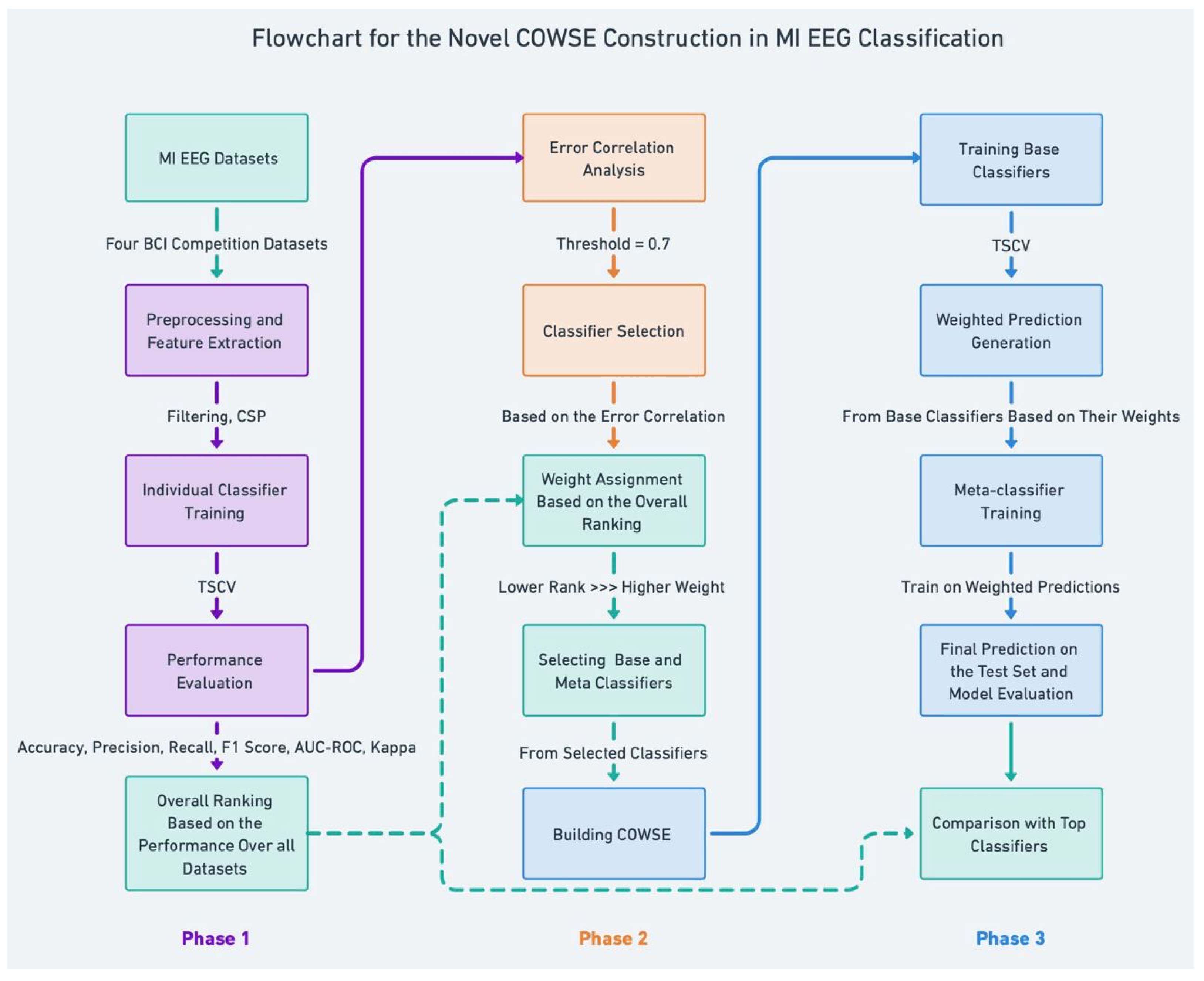
In crafting our ensemble model, Correlation-Optimized Weighted Stacking Ensemble (COWSE) signifies a leap in MI EEG classification. We delineate a multi-stage process in Figure 1 that begins with error correlation analysis. This step is crucial as it informs the selection of diverse base classifiers, directly contributing to an ensemble greater than the sum of its parts. Subsequent weight assignment uniquely correlates to each classifier’s rank, inversely allocating weight and fostering a novel dynamic within the ensemble.

Central to our method is the COWSE construction, an innovative composite weighted ensemble that distinctly characterizes our research. This step is depicted in phase 2 of Figure 1, where the strategic selection and weighting of classifiers are based on a newfangled analysis of error patterns, a step that deviates from conventional ensemble methods.

Phase 3 encapsulates the meta-classifier training predicated on these weighted predictions. This unique aspect of our work harnesses the collective strengths of individual classifiers, thereby constructing a more sophisticated predictive model. Our approach diverges from traditional ensembles by prioritizing classifier diversity and dynamic weight adjustment, which are informed by performance metrics, thus introducing an error correlation analysis and a novel weight assignment mechanism.

This strategic approach, particularly evident in classifier selection and meta-classifier training, sets our method apart. We leverage a deeper analysis of error patterns and classifier performance, which are often overlooked in existing frameworks, to enhance the robustness and accuracy of MI EEG classification.

2.5.1. Classifier Selection Based on Error Correlation

The first step in constructing the ensemble model involves selecting a subset of classifiers based on their performance and error correlation across the datasets. For this purpose, we define the error vector, $er{r}_i$, for classifier i as a vector, where each element corresponds to the binary classification outcome for each instance in the dataset, with ‘1’ indicating a misclassification and ‘0’ indicating a correct classification. The error correlation matrix, E, is computed as follows:

$$E_{i,j}=\mathrm{corr}(er{r}_i,er{r}_j)$$

(1)

where $er{r}_i$ and $er{r}_j$ represent the error vectors of classifiers i and j across all the datasets, respectively. The correlation coefficient, $\mathrm{corr}(·)$, measures how similarly classifiers i and j misclassify samples. Classifiers with lower average correlation coefficients are selected to ensure diversity in the ensemble.

2.5.2. Weight Assignment Based on Performance Ranking

Upon selecting base classifiers, we assign weights to each by adjusting a sensitivity parameter $\alpha$, which governs the distribution of weights according to the classifiers’ performance ranks across datasets. The weight for classifier i, $w_i$, is computed as

$$w_i=\frac{1}{{\mathrm{rank}}_i^{\alpha }}$$

(2)

where ${\mathrm{rank}}_i$ indicates the performance rank of classifier i and $\alpha$ modulates the weight distribution. A higher $\alpha$ emphasizes the contribution of top-ranked classifiers by penalizing lower-ranked ones more severely.

To optimize $\alpha$, we employ Bayesian Optimization, which models the ensemble’s performance as a function of $\alpha$ using a Gaussian Process (GP). The GP, characterized by its mean function $m\left(x\right)$ and covariance function $k(x,x^{\prime })$, provides a probabilistic performance prediction for any given $\alpha$.

The ensemble’s performance, modeled as a function of $\alpha$, is provided by

$$P\left(\alpha \right)=m\left(\alpha \right)+ϵ,ϵ\sim N(0,k(\alpha ,{\alpha }^{\prime }))$$

(3)

where $P\left(\alpha \right)$ is the predicted performance, $m\left(\alpha \right)$ is the mean function of the GP, and $ϵ$ represents the noise in the prediction, modeled as a Gaussian distribution, with zero mean and variance determined by the covariance function $k(\alpha ,{\alpha }^{\prime })$.

The optimization process is guided by an acquisition function, which we define as

$$A\left(\alpha \right)=\mu \left(\alpha \right)+\kappa \sigma \left(\alpha \right)$$

(4)

where $A\left(\alpha \right)$ is the acquisition function value for a given $\alpha$, $\mu \left(\alpha \right)$ and $\sigma \left(\alpha \right)$ are the mean and standard deviation of the GP’s prediction for $\alpha$, respectively, and $\kappa$ is a parameter that balances exploration and exploitation.

The optimization problem to find the optimal $\alpha$ that maximizes the ensemble’s performance is formulated as

$${\alpha }^{*}=arg\underset{\alpha }{max}A\left(\alpha \right)$$

(5)

This approach systematically navigates the parameter space of $\alpha$, identifying the value that optimizes ensemble performance with minimal computational effort. By optimizing the acquisition function, we ensure the selection of an $\alpha$ that achieves an optimal balance in classifier weight distribution, enhancing the ensemble model’s predictive accuracy.

2.5.3. Stacking with Meta-Classifier

The ensemble model utilizes a stacking approach, where a meta-classifier is trained on the predictions of the base classifiers. Let X denote the feature matrix of the original dataset and Y the corresponding target vector. The base classifiers produce a new feature matrix, Z, for the meta-classifier, where each row, $z_n$, corresponds to the weighted predictions of the base classifiers for sample n:

$$z_{n,i}=w_i·p_{n,i}$$

(6)

where $p_{n,i}$ is the prediction of the ith base classifier for the nth sample. The meta-classifier is then trained on Z with the target Y, learning to combine the base classifiers’ weighted predictions optimally.

The final prediction, ${\widehat{y}}_n$, for a sample n is obtained by

$${\widehat{y}}_n=\mathrm{meta}-\mathrm{classifier}\left(z_n\right)$$

(7)

where $\mathrm{meta}-\mathrm{classifier}(·)$ denotes the prediction function of the meta-classifier.

3. Results

In this section, we present the outcomes of our comprehensive experimental evaluations. The analysis commences with an overarching comparison of the classifier performance across all four datasets. Each classifier’s effectiveness is quantified through various metrics, an overall score, and their corresponding rank based on these metrics. The results aim to provide a foundational understanding of each classifier’s initial performance before applying our ensemble model construction methodology.

Table 3. Comparison of the classifiers based on their performance on the BNCI2014-001 dataset [25].

Classifier	Accuracy	Precision	Recall	F1-Score	AUC-ROC	Kappa	Score	Rank
MLP	0.7694	0.7715	0.7694	0.7690	0.8465	0.6925	0.7697	1
SVM-rbf	0.7659	0.7694	0.7659	0.7654	0.8444	0.6879	0.7665	2
LR	0.7070	0.7076	0.7070	0.7055	0.8048	0.6091	0.7068	3
SVM	0.7054	0.7091	0.7054	0.7047	0.8041	0.6077	0.7061	4
LDA	0.6951	0.6967	0.6951	0.6939	0.7969	0.5934	0.6952	5
QDA	0.6561	0.6590	0.6561	0.6548	0.7696	0.5409	0.6561	6
ET	0.6533	0.6595	0.6533	0.6516	0.7683	0.5375	0.6539	7
RC	0.6542	0.6560	0.6542	0.6506	0.7679	0.5378	0.6534	8
GB	0.6322	0.6387	0.6322	0.6320	0.7534	0.5093	0.6330	9
RF	0.6293	0.6349	0.6293	0.6293	0.7516	0.5055	0.6300	10
SGD	0.6255	0.6476	0.6255	0.6097	0.7509	0.5007	0.6266	11
KN	0.6188	0.6354	0.6188	0.6194	0.7456	0.4922	0.6217	12
NB	0.6073	0.6105	0.6073	0.6025	0.7360	0.4755	0.6065	13
PC	0.5852	0.6452	0.5852	0.5556	0.7219	0.4448	0.5896	14
DT	0.5623	0.5669	0.5623	0.5612	0.7070	0.4155	0.5625	15
AB	0.5517	0.5659	0.5517	0.5469	0.6992	0.4007	0.5527	16

,

Table 4. Comparison of the classifiers based on their performance on the BNCI2014-002 dataset [26].

Classifier	Accuracy	Precision	Recall	F1-Score	AUC-ROC	Kappa	Score	Rank
SVM_rbf	0.9220	0.9235	0.9220	0.9220	0.9221	0.8436	0.9092	1
MLP	0.8878	0.8884	0.8878	0.8877	0.8874	0.7747	0.8690	2
SVM	0.8750	0.8770	0.8750	0.8750	0.8753	0.7497	0.8545	3
LR	0.8708	0.8720	0.8708	0.8708	0.8708	0.7409	0.8493	4
LDA	0.8683	0.8704	0.8683	0.8682	0.8685	0.7361	0.8466	5
RC	0.7723	0.7846	0.7723	0.7724	0.7758	0.5440	0.7369	6
NB	0.7723	0.7838	0.7723	0.7721	0.7760	0.5426	0.7365	7
SGD	0.7634	0.7735	0.7634	0.7564	0.7640	0.5203	0.7235	8
KN	0.7545	0.7708	0.7545	0.7546	0.7608	0.5117	0.7178	9
GB	0.7522	0.7680	0.7522	0.7518	0.7571	0.5059	0.7145	10
PC	0.7522	0.7648	0.7522	0.7520	0.7561	0.5039	0.7135	11
AB	0.7500	0.7643	0.7500	0.7501	0.7545	0.4989	0.7113	12
QDA	0.7478	0.7572	0.7478	0.7482	0.7505	0.4930	0.7074	13
DT	0.7455	0.7515	0.7455	0.7447	0.7454	0.4844	0.7028	14
RF	0.7210	0.7543	0.7210	0.6900	0.7285	0.4505	0.6775	15
ET	0.7143	0.7200	0.7143	0.7141	0.7153	0.4257	0.6673	16

,

Table 5. Comparison of the classifiers based on their performance on the BNCI2014-004 dataset [27].

Classifier	Accuracy	Precision	Recall	F1-Score	AUC-ROC	Kappa	Score	Rank
SVM_rbf	0.7627	0.7635	0.7627	0.7621	0.7619	0.5238	0.7228	1
MLP	0.7585	0.7599	0.7585	0.7583	0.7583	0.5164	0.7183	2
LR	0.7475	0.7483	0.7475	0.7474	0.7471	0.4939	0.7053	3
SVM	0.7464	0.7479	0.7464	0.7461	0.7465	0.4924	0.7043	4
LDA	0.7444	0.7454	0.7444	0.7443	0.7442	0.4878	0.7017	5
QDA	0.7304	0.7371	0.7304	0.7289	0.7320	0.4618	0.6868	6
RC	0.7290	0.7360	0.7290	0.7282	0.7314	0.4605	0.6857	7
RF	0.7267	0.7311	0.7267	0.7267	0.7278	0.4536	0.6821	8
GB	0.7265	0.7310	0.7265	0.7266	0.7277	0.4535	0.6820	9
NB	0.7173	0.7226	0.7173	0.7161	0.7183	0.4348	0.6711	10
AB	0.7079	0.7140	0.7079	0.7071	0.7104	0.4186	0.6610	11
KN	0.7081	0.7116	0.7081	0.7082	0.7081	0.4152	0.6599	12
ET	0.7072	0.7111	0.7072	0.7075	0.7076	0.4138	0.6591	13
DT	0.6945	0.6981	0.6945	0.6942	0.6939	0.3875	0.6438	14
PC	0.6964	0.6855	0.6964	0.6498	0.6911	0.3830	0.6337	15
SGD	0.6736	0.6955	0.6736	0.6300	0.6820	0.3634	0.6197	16

and

Table 6. Comparison of the classifiers based on their performance on the BNCI2015-001 dataset [28].

Classifier	Accuracy	Precision	Recall	F1-Score	AUC-ROC	Kappa	Score	Rank
SVM_rbf	0.8908	0.8917	0.8908	0.8908	0.8908	0.7815	0.8727	1
MLP	0.8765	0.8769	0.8765	0.8764	0.8763	0.7526	0.8559	2
SVM	0.8603	0.8612	0.8603	0.8603	0.8603	0.7205	0.8371	3
LR	0.8568	0.8575	0.8568	0.8568	0.8567	0.7134	0.8330	4
LDA	0.8522	0.8532	0.8522	0.8521	0.8522	0.7042	0.8277	5
RF	0.8226	0.8271	0.8226	0.8220	0.8232	0.6447	0.7937	6
ET	0.8222	0.8263	0.8222	0.8218	0.8231	0.6442	0.7933	7
KN	0.8201	0.8248	0.8201	0.8197	0.8215	0.6407	0.7911	8
RC	0.8191	0.8216	0.8191	0.8190	0.8195	0.6379	0.7894	9
GB	0.8146	0.8178	0.8146	0.8145	0.8157	0.6294	0.7844	10
AB	0.8090	0.8121	0.8090	0.8090	0.8096	0.6180	0.7778	11
QDA	0.7948	0.8007	0.7948	0.7928	0.7957	0.5899	0.7614	12
NB	0.7917	0.8081	0.7917	0.7839	0.7920	0.5826	0.7583	13
DT	0.7771	0.7796	0.7771	0.7764	0.7772	0.5537	0.7402	14
SGD	0.7660	0.8010	0.7660	0.7557	0.7696	0.5363	0.7324	15
PC	0.7535	0.8181	0.7535	0.7228	0.7578	0.5155	0.7202	16

detail the comparative performance of the classifiers across the respective datasets, laying the groundwork for further analysis and discussion on the ensemble model’s efficacy.

Although we assessed the classifiers on a multitude of metrics, the initial visual comparison is focused on accuracy due to its fundamental role in performance evaluation. Each classifier’s accuracy was calculated as an average across all the subjects within each dataset, ensuring a thorough representation of performance across varying conditions. Figure 2 showcases these accuracy values, delineating individual and average performance metrics, which form the basis for ranking the classifiers, a critical step in developing our ensemble model.

Upon completing the individual analyses of each dataset, we amalgamate the findings to present a holistic view of the classifiers’ performance.

Table 7. Overall ranking of classifiers based on composite scores for ensemble integration.

Classifier	SVM_rbf	MLP	SVM	LR	LDA	RC	GB	QDA	KN	RF	ET	NB	AB	SGD	PC	DT
Score	0.819	0.803	0.775	0.774	0.769	0.716	0.703	0.703	0.698	0.696	0.693	0.693	0.676	0.675	0.664	0.662
Rank	1	2	3	4	5	6	7	8	9	10	11	12	13	14	15	16

consolidates these insights, presenting a unified ranking that reflects a composite score for each classifier across all the datasets.

Following the initial performance evaluation, it is essential to explore how the classifiers’ errors relate to one another. This understanding informs the selection of diverse classifiers for the ensemble, aiming to minimize overlapping weaknesses. The error correlation matrix, illustrated in Figure 3, visually represents the relationships between classifier error rates. A lower correlation (indicated in blue) suggests that classifiers make errors on different samples, while a higher correlation (shown in red) means they err on similar instances.

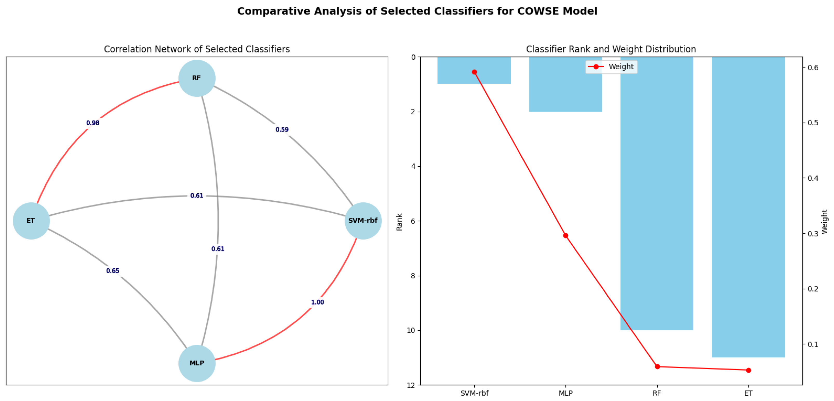
Observations from the error correlation matrix indicate that certain classifiers exhibit lower correlation in their error rates, suggesting a potential for greater diversity in an ensemble model. Four classifiers—SVM-rbf, MLP, RF, and ET—demonstrated the lowest pairwise correlation rates compared to the others, as summarized in Figure 4. In contrast, all the other pairs showed a correlation rate above 0.7. Consequently, based on this criterion for diversity, SVM-rbf, MLP, RF, and ET were selected as the constituents of the ensemble model.

Optimizing classifier weights was crucial in enhancing the COWSE model’s performance. Through applying Bayesian Optimization, we determined the optimal value of the weight distribution sensitivity parameter, $\alpha$, to be 1.229. This rigorous optimization process utilized a GP to model the ensemble’s performance as a function of $\alpha$, incorporating both the mean performance prediction and the variance to systematically explore and exploit the parameter space. The optimal $\alpha$ value achieved reflects a sophisticated balance in the weight distribution among the classifiers and underscores our optimization strategy’s effectiveness in enhancing the ensemble’s predictive accuracy.

The optimal $\alpha$ value was then applied in Equation (2) to ascertain the weights for each selected classifier within the COWSE model. Consequently, SVM-rbf was allotted the heaviest weight of 0.592, reflecting its superior rank. Following suit, MLP, RF, and ET were assigned weights of 0.296, 0.059, and 0.053, respectively. These calculated weights are depicted in Figure 4, illustrating the balanced contribution of each classifier to the ensemble, a testament to the harmonized synergy within the COWSE model.

This recalibration significantly influenced the ensemble’s weight distribution, allowing us to leverage the strengths of higher-performing classifiers while maintaining the diversity contributed by the entire classifier pool. Adopting the optimized $\alpha$ value led to a noticeable improvement in the ensemble model’s overall accuracy, as demonstrated by comparative analyses against baseline models. The results underscore the importance of precise parameter optimization in ensemble models, confirming the efficacy of our approach in refining the COWSE model’s predictive performance.

Following the selection process informed by the error correlation matrix, we constructed the COWSE model, integrating SVM-rbf, MLP, RF, and ET classifiers. The performance of the COWSE model across all the datasets is presented in

Table 8. Performance of COWSE over all datasets.

Dataset	Accuracy	Precision	Recall	F1-Score	AUC-ROC	Kappa
BNCI2014-001	0.9601	0.9602	0.9601	0.9601	0.9733	0.9467
BNCI2014-002	0.9816	0.9818	0.9816	0.9816	0.9878	0.9754
BNCI2014-004	0.9366	0.9388	0.9366	0.9366	0.9371	0.8732
BNCI2015-001	0.9775	0.9781	0.9775	0.9775	0.9771	0.9550

.

To visually compare the performance of our ensemble model with that of the top-performing individual classifiers, a bar chart is presented in Figure 5. This comparison highlights the advantages of the COWSE model in terms of accuracy across all the datasets, offering an intuitive understanding of the ensemble model’s improved prediction capability.

4. Discussion

In this section, we interpret the results of our experiments and discuss their implications for the field of MI EEG classification. We begin by reflecting on the comparative analysis of classifier performance and proceed to the significance of our error correlation approach and the construction of the COWSE.

4.1. Interpretation of Classifiers’ Performance in the Initial Phase

The detailed comparative analysis of classifier accuracy values presented in Figure 2 reveals patterns of consistency and variability across different MI EEG datasets and underscores the hierarchical positioning of certain classifiers. Classifiers such as SVM-rbf, MLP, SVM, LR, and LDA demonstrate robustness, consistently ranking within the top five performers and frequently surpassing the average accuracy. This indicates their general efficacy and reliability in handling EEG data.

In contrast, classifiers like DT and PC consistently rank as some of the least effective, falling among the bottom performers across all the datasets examined. This persistent underperformance suggests inherent limitations in their ability to model EEG data complexities within this analysis’s scope. Meanwhile, classifiers such as RC and GB exhibit moderate performance, neither excelling nor failing significantly but maintaining a steady middle ground.

Conversely, classifiers like QDA and ET show observable variability, ranking fluctuations across datasets, and sensitivity to dataset-specific characteristics. Such insights are instrumental for developing ensemble methods as they highlight the potential benefit of combining consistently high performers with those tailored to exploit dataset-specific features, thus achieving a balance between stability and adaptability in model performance.

The synthesis of results into a comprehensive overview, as presented in Table 7, is pivotal in our ensemble model construction. By establishing a foundational ranking system based on a composite score, we ensure a balanced approach to model integration. This system objectively encapsulates the multi-metric performance of classifiers, reflecting their overall efficacy rather than relying on a single metric. Such an approach provides a holistic view of classifier capabilities, guiding the weighted contributions of each classifier in the ensemble model. The weighting scheme, derived from these rankings, is designed to provide precedence to classifiers with superior overall performance while valuing the unique contributions of lower-ranked classifiers.

4.2. Leveraging Error Correlation to Fortify Ensemble Robustness

The distribution of classifier performance necessitates further investigation into the error patterns of individual models. By understanding when and how often classifiers make mistakes and the nature of these errors, we can more strategically construct ensemble models that are greater than the sum of their parts. It is here that error correlation analysis becomes invaluable.

The error correlation matrix, as shown in Figure 3, provides critical insight into the error patterns of classifiers. Classifiers with low error correlation rates indicate diverse error patterns, implying that, when one classifier misclassifies an instance, the other will likely classify it correctly. This diversity is the linchpin of a robust ensemble model as it allows for the mutual compensation of individual classifier weaknesses. Therefore, the strategic selection of classifiers with the least error correlation for our COWSE model—specifically SVM-rbf, MLP, RF, and ET—was informed by the intent to leverage this diversity to its fullest potential. In selecting SVM-rbf, MLP, RF, and ET, our focus was on the lowest error correlation pairs available, which were found to be between SVM-rbf and RF, SVM-rbf and ET, MLP and RF, and MLP and ET.

While higher error correlations are present between SVM-rbf and MLP and between RF and ET, these are not detrimental to the ensemble’s efficacy. The strength of SVM-rbf in high-dimensional space mapping is effectively complemented by MLP’s proficiency in capturing non-linear relationships, which cover a wider array of data patterns. Similarly, the RF and ET classifiers, by their distinct approaches to decisionmaking—RF with its bootstrapped samples and ET with its complete dataset—provide a multifaceted view of the data. This intentional overlap in capabilities ensures that the ensemble can tackle complex classification scenarios where a single model’s perspective is insufficient.

The COWSE model’s outstanding performance across various datasets illustrates the soundness of our selection strategy. We have established a robust model capable of superior performance by focusing on the pairs with the lowest error correlations for ensemble integration. The success of the COWSE model underscores our methodical approach to ensemble construction, which emphasizes the strategic balance of classifier strengths to achieve optimal classification results.

4.3. Visualising the Correlation Network and Rank-Weight Dynamics in COWSE

The strategic selection of classifiers for the COWSE model is visually encapsulated in Figure 4. The network diagram on the left side of the figure illustrates the error correlation network among the selected classifiers. The edges connecting the classifiers are labeled with pairwise correlation values, highlighting the low error correlation pivotal to their synergistic strength within the ensemble. The decision to include classifiers with the least error correlation—SVM-rbf, MLP, RF, and ET—was propelled by the intent to capitalize on this diversity, thereby enhancing the robustness and accuracy of the ensemble model.

Complementing the network diagram, the bar chart on the right side delineates each classifier’s rank and weight distribution, illustrating the inverse relationship between a classifier’s rank and its weight within the COWSE model. The overlay line graph clearly shows that, while the SVM-rbf stands as the top-ranked classifier and thus holds the highest weight, the subsequent classifiers are weighted in descending order according to their rank. This weight distribution is integral to the ensemble’s decisionmaking process, ensuring that each classifier’s contribution is proportional to its demonstrated performance yet preserves the ensemble’s ability to benefit from the collective diversity.

4.4. Rationale behind Diverse Classifier Integration in COWSE

• Strategic Balance Between Performance and Diversity: High-performing classifiers, such as SVM-rbf and MLP, offer proven reliability and accuracy, serving as strong pillars within the ensemble. However, their strengths alone do not fully encapsulate the diversity of error patterns necessary for a comprehensive ensemble model. By including classifiers like RF and ET, which may not top the performance charts but exhibit unique error characteristics, we introduced a heterogeneity level essential for ensemble robustness.
• Leveraging Complementary Error Patterns: Including lower-ranked classifiers is not arbitrary; it is informed by the error correlation analysis, which identifies classifiers that make uncorrelated errors. Such classifiers can complement the decisionmaking of the ensemble, ensuring that the model does not echo the mistakes of its components but rather learns from them.
• Weighted Contribution Based on Performance: While we acknowledge the value of diverse classifiers, we maintain a performance-oriented approach by weighting them according to their ranks, as indicated by Figure 4. This ensures that the contributions of higher-performing classifiers are prioritized, aligning with their demonstrated ability to handle EEG data effectively. However, the weights are calibrated to ensure that the ensemble benefits from the full spectrum of classifier capabilities, achieving a balance between reliability and comprehensive error representation.
• Ensuring Systematic and Objective Ensemble Construction: Our approach is systematic and objective, grounded in empirical data rather than arbitrary selection. This method ensures that the ensemble is constructed on the principle of diversity and a quantifiable measure of performance and error correlation. It is a nuanced balance that maximizes each classifier’s strengths while safeguarding against weaknesses.

4.5. Constructing the COWSE Model

The COWSE model employs a nuanced blend of weighting and stacking methodologies to create a robust ensemble for MI EEG classification.

4.5.1. Base Classifiers

The COWSE model integrates four classifiers—SVM-rbf, MLP, RF, and ET—each assigned a weight corresponding to their performance ranking (Figure 4). SVM-rbf, the highest-ranked classifier, is accorded the most substantial weight of 0.592, establishing it as the primary contributor to the ensemble’s predictions. Although MLP has a lower rank than SVM-rbf with a weight of 0.296, it serves a dual function: it is a significant base classifier and acts as the meta-classifier, orchestrating the ensemble’s output. RF and ET, although carrying lighter weights of 0.059 and 0.053, are integral to the model, adding depth and breadth to the ensemble’s decisionmaking capabilities. Together, this quartet forms the robust COWSE model, their respective weights ensuring a dynamic balance between individual accuracy and collective strength.

4.5.2. Choosing MLP as the Meta-Classifier: A Strategic Decision

In the COWSE model, the meta-classifier role is assigned to MLP, a decision driven by its robust pattern recognition abilities and proficiency in integrating diverse outputs. The rationale behind this choice is as follows:

• Capability to Model Non-linear Relationships: MLPs are renowned for their ability to capture and model non-linear relationships within data. EEG signals are inherently complex and non-linear, often requiring a model that can navigate through this non-linearity to make accurate predictions. MLPs, with their layered structure and non-linear activation functions, provide the necessary framework to decipher these intricate patterns and relationships that are not explicitly defined.
• Harnessing Diverse Classifier Outputs: The role of a meta-classifier is to predict and synthesize diverse information presented by base classifiers. An MLP is adept at integrating these varied outputs, learning from each classifier’s successes and shortcomings. This process involves recognizing patterns in how classifiers complement each other’s predictions, which is crucial for the ensemble’s performance.
• Flexibility and Customization: MLPs offer a high degree of flexibility, allowing for the customization of their architecture to suit the specific needs of the task. This adaptability is critical when dealing with diverse datasets as it enables the MLP model to be tuned for the particularities of each dataset, ensuring that the ensemble remains effective across various EEG data configurations.
• Generalization Across Varied Conditions: In the context of EEG classification, it is paramount that the meta-classifier generalizes well to new data, including different subjects and sessions. MLPs have demonstrated this ability, particularly when regularization techniques are employed. This ensures that the ensemble model constructed is precise but also robust and reliable under varying conditions.
• Expertise in BCI Applications: MLPs have a long-standing reputation and a proven track record in BCI applications. Their widespread use and the substantial body of research supporting their effectiveness provide a strong foundation for their role as meta-classifiers, suggesting that MLP can handle the unique challenges of BCI tasks, including classifying MI EEG signals.
• Empirical Validation: Beyond the theoretical advantages, we conducted empirical tests comparing the performance of MLP and SVM-rbf as the meta-classifier. These tests revealed that the ensemble model with MLP as the meta-classifier consistently achieved higher accuracy and performance metrics than when SVM-rbf was used. This empirical evidence further solidified our decision to designate MLP as the meta-classifier, ensuring the ensemble’s optimal performance.

In optimizing the COWSE model, we carefully tuned the hyperparameters of each classifier using a grid search for SVM-rbf due to its simpler parameter space and random search for MLP, RF, and ET to explore their complex parameter spaces efficiently. Our tuning process focused on computational efficiency, employing multiple performance metrics, and used TSCV for robust validation across time-varying data. We also considered parameter range, scale, and data characteristics to ensure our hyperparameter choices were well-suited to the data. The resulting configurations are detailed in

Table 9. Hyperparameters for SVM-RBF, MLP, RF, and ET classifiers.

Classifier	Hyperparameter	Value
SVM-RBF	C (Regularization parameter)	1
MLP	Number of layers and size	1 hidden layer, 150 neurons
	Activation function	ReLU
	Learning rate	0.001
	Regularization	L2 (0.0001), Dropout (0.5)
RF	Number of trees	100
	Max depth of trees	None
	Min samples split	2
	Max features	sqrt
ET	Number of trees	100
	Max depth of trees	None
	Min samples split	2
	Max features	auto
	Bootstrap	False

.

4.6. Training and Evaluation of the COWSE Model

The COWSE model employs a rigorous training regimen grounded in TSCV, a strategic choice reflecting an acute awareness of the temporal dependencies in EEG data. During the initial training phase, base classifiers undergo meticulous training across multiple folds. To ensure the most comprehensive learning and validation process, we determined the optimal number of folds to be eight through a grid search optimization process. This ensures a comprehensive learning process wherein each classifier’s hyperparameters are fine-tuned for optimal performance. The optimization algorithms intrinsic to each classifier, as employed by the siket-learn library, guide this fine-tuning process. For instance, SVM utilizes a Sequential Minimal Optimization (SMO) algorithm for training, while tree-based classifiers such as RF and ET leverage an ensemble of Decision Trees.

For the MLP classifier, the training process is based on backpropagation, a method that efficiently calculates the gradient of the loss function. Specifically, MLP employs the cross-entropy loss function to quantify the difference between the predicted probabilities and the actual class labels, making it highly suitable for classification tasks. This loss function handles multiple classes and ensures that the model’s predictions closely align with the true outcomes. Additionally, MLP utilizes the Adam optimizer, renowned for its effectiveness in adjusting the learning rate during training, which helps converge to the optimal solution more efficiently and effectively. This combination of cross-entropy loss and Adam optimizer allows MLP to learn complex patterns in the data, contributing significantly to the ensemble’s predictive performance.

Following the base training, a unique feature of COWSE emerges—the construction of a meta-classifier. This step involves weighting the base classifiers’ predictions to form a new feature matrix, a process where the ensemble’s collective intelligence is harnessed. The weighting mechanism is proportional to each classifier’s performance, ensuring that more accurate classifiers exert greater influence on the final prediction.

The MLP meta-classifier integrates these weighted predictions as the ensemble’s synthesis point. It is trained on this composite feature matrix, embodying the collective insights of the base classifiers. MLP’s learning process, guided by the cross-entropy loss function and optimized by the Adam optimizer, minimizes prediction error, enhancing the ensemble’s predictive accuracy.

The true measure of COWSE’s prowess is reflected in its performance against unseen data. The model’s evaluation on the separate testing set reveals its capability to generalize beyond the training data, a testament to its robust construction and the validity of the TSCV training approach. Table 8 shows that the comparative analysis confirms COWSE’s superiority across all the datasets. The application of TSCV in both base and meta-classifier training phases ensures a rigorous and thorough validation process, reinforcing the model’s validity and robustness.

The comprehensive performance of the ensemble model is visually represented in Figure 5, where the accuracy of COWSE is benchmarked against the top six individual classifiers. The bar chart elucidates the ensemble’s superiority, highlighting how the correlation-optimized approach in ensemble construction pays dividends in predictive performance.

4.7. Comparison with Related Works

Our COWSE model showcases remarkable advancements in MI EEG signal classification, leveraging a unique ensemble learning strategy that combines weighted averaging, stacking approaches, error correlation analysis, and adaptive methodologies, as illustrated in

Table 10. Performance comparison of COWSE model with related works.

Refrence	Classifiers	Datasets	Ensemble Methods	Accuracy
Nicolas et al., 2014 [19]	LDA	1	Stacking	85.64%
Rahimi et al., 2016 [21]	SVM, LDA, DT	1	Stacking	90.18%
Ramos et al., 2017 [18]	SVM, KN, LDA	2	Weighted, Adaptive	97.02%
Raza et al., 2019 [31]	AB	2	Weighted, Adaptive	81.79%
Rashid et al., 2021 [22]	RF, KN, LDA, SVM	4	Weighted	99.21%
Zheng et al., 2021 [24]	SVM	1	Weighted	82.91%
Chen et al., 2022 [32]	RF, GB, DT, LR	1	Stacking	90.73%
This Study	LDA, QDA, RF, SVM, LR, NB, KN, RC, DT, GB, ET, MLP, SVM-rbf, SGD, AB, PC	4	Weighted, Stacking, Error Correlation Analysis, Adaptive	98.16%

. This multifaceted approach has not been paralleled in the existing literature, particularly in employing weighted and stacking methods alongside error correlation analysis to construct the ensemble model. While ensemble learning has been explored in MI EEG classification, the depth and complexity of our model set a new benchmark for accuracy and robustness.

Among the related works, Rashid et al. [22] reported a notable 99.21% accuracy on the BNCI2014-002 dataset using an ensemble of four classifiers (RF, KN, LDA, and SVM) without integrating the advanced techniques utilized in our COWSE model. Our COWSE model, in contrast, achieved a commendable 98.16% accuracy on the same dataset. Importantly, it outperformed Rashid et al.’s approach across the other three datasets—BNCI2014-001, BNCI2014-004, and BNCI2015-001—with accuracy values of 96.01%, 93.66%, and 97.75%, respectively, as detailed in Table 8. In comparison, they achieved 93.19%, 93.57%, and 90.32% on these datasets. Despite their higher accuracy on one dataset, this comparison demonstrates that our COWSE model consistently outperforms most datasets, affirming its superiority and robustness in MI EEG signal classification.

The key distinctions between our work and the related studies include the following:

• Classifier Diversity: Our model’s incorporation of 16 diverse classifiers enhances data feature representation and classification robustness.
• Methodological Innovations: The combination of error correlation analysis with weighted and stacking ensemble methods in our COWSE model provides a novel approach to MI EEG signal classification, surpassing the traditional ensemble strategies used in prior studies.

These distinctions highlight the comprehensive and innovative nature of our COWSE model. Adopting a multilayered ensemble strategy incorporating weighted predictions, stacking, error correlation analysis, and adaptive methods, our model sets a new benchmark for accuracy and robustness in MI EEG signal classification.

4.8. Adaptability and Implications of the COWSE Model for Diverse Datasets

The flexibility embedded within the COWSE model allows for its application across various datasets, which may exhibit differences in signal quality, task design, subject variability, and data distribution. This adaptability is crucial for advancing BCI technologies to cater to various applications and user needs. To illustrate this adaptability, we highlight key areas where the COWSE model excels:

• Signal Quality: Variations in signal-to-noise ratio and the presence of artifacts are mitigated through our rigorous preprocessing and feature extraction steps, ensuring the model’s robustness.
• Task Design and Subject Variability: The ensemble approach, leveraging multiple classifiers, captures various discriminative features, thereby accommodating different MI tasks and reducing susceptibility to inter-subject variability. For instance, when applied to datasets from subjects with varying levels of BCI proficiency, the COWSE model demonstrated the ability to maintain high classification accuracy, showcasing the ensemble’s effectiveness in capturing diverse cognitive patterns.
• Data Distribution: The model’s weighting scheme handles imbalanced datasets by dynamically adjusting classifier influence based on performance, ensuring equitable representation of all classes.

When adapting the COWSE model to a significantly different dataset, several implications must be considered:

• Preprocessing Re-evaluation: Adjustments to the preprocessing pipeline may be necessary to cater to new dataset characteristics, such as differing artifact types or frequency bands.
• Feature Space Exploration: The feature extraction process may need revisiting to capture the most informative features for the new dataset, ensuring optimal model performance.
• Hyperparameter Retuning: Individual classifiers and the ensemble model itself may require hyperparameter adjustments to align with new data characteristics, optimizing classification accuracy.
• Validation Approach Modification: To prevent overfitting and ensure generalization, the cross-validation strategy might need adaptation based on the new dataset’s size and composition.
• Performance Metrics Reassessment: The selection of performance metrics should be revisited to ensure that they remain relevant and indicative of successful classification in the context of the new dataset.

Moreover, integrating with other data modalities, such as fNIRS or ECoG, could further enhance the model’s applicability and robustness. This innovative approach to adaptation demonstrates the model’s versatility and paves the way for its application in a wider range of BCI-related tasks, potentially extending beyond EEG classification.

By addressing these aspects, the COWSE model’s adaptability ensures its efficacy across diverse settings, significantly advancing personalized and accurate BCI systems.

4.9. Limitations and Future Research Directions

The COWSE model has demonstrated its potential to significantly impact the field of BCI, particularly in the domain of MI EEG classification. Its adaptability and robustness across various MI EEG classification tasks underscore its value. However, as we venture beyond its current applications, it becomes crucial to address certain limitations and identify directions for future research that could further refine and expand its utility.

4.9.1. Limitations

• Computational Complexity: Integrating multiple classifiers and an advanced weighting mechanism contributes to the model’s high computational demand. Future initiatives must focus on balancing this complexity with the necessity for maintaining or enhancing classification accuracy.
• Real-World Applicability: The deployment of the COWSE model in real-life BCI applications requires rigorous testing, especially in environments characterized by complex and unpredictable noise patterns. Enhancing the model’s robustness in such conditions remains a priority.
• Adaptability to User Variability: The efficacy of BCI systems significantly depends on their ability to adapt to individual differences among users. Investigating the COWSE model’s flexibility in adjusting to these user-specific characteristics is essential for its success in practical applications.

4.9.2. Future Research Directions

• Optimization Strategies: Exploring methods to reduce the model’s computational load without compromising its effectiveness is a critical step forward. This could involve algorithmic optimizations or more efficient classifier integration techniques.
• Preprocessing and Feature Extraction: Assessing the impact of various data preprocessing and feature extraction methods could unveil opportunities to enhance the model’s performance across diverse datasets.
• Expanding Classifier Ensemble: Incorporating additional classifiers or refining the ensemble strategy could provide new insights into achieving higher classification accuracy and better generalizability.
• Personalization and Real-Time Performance: Future studies should aim to tailor BCI systems to individual users and evaluate the COWSE model in real-time scenarios to ensure its viability for everyday applications.
• Exploring Deep Learning (DL) Methodologies: Additionally, while our current exploration within the COWSE model focuses on traditional ML approaches, there is a growing recognition of DL methodologies’ potential in enhancing BCI systems. DL’s capacity for automated feature extraction, scalability, and proficiency in handling complex high-dimensional datasets present a promising frontier for BCI research. However, applying DL in this context is not without challenges. The substantial volume of data required to train DL models, alongside concerns regarding model interpretability and computational demands, necessitate careful consideration. Future research could explore integrating DL techniques to complement the COWSE model, potentially revealing a path to overcoming the existing limitations and unlocking new capabilities in BCI technology.

We can further solidify the COWSE model’s foundational role in advancing BCI technology by addressing these limitations and pursuing the outlined research directions. These efforts promise to enhance the model’s current capabilities and open new avenues for personalized and efficient BCI solutions.

5. Conclusions

In conclusion, the COWSE model represents a significant leap in MI EEG signal classification, setting a new standard regarding accuracy and adaptability. It underscores the potential of diverse classifier ensembles to boost performance. Despite these advances, we acknowledge the inherent challenges in EEG signal classification, such as decoding complex brain signals, variability in signal quality across individuals, and the limitations these factors may impose on the model’s reliability and applicability. Future research should address computational demands, enhance real-world robustness, and adapt more closely to user variability. Optimization strategies, advanced preprocessing, and feature extraction methods are envisaged. The key next steps are expanding the classifier ensemble and customizing systems for real-time personalized use. The model’s implications for healthcare monitoring and assistive technologies highlight the need for interdisciplinary collaborations and user-centered design to make BCI technologies more accessible and tailored to diverse needs. Acknowledging these uncertainties and limitations adds depth to our understanding and paves the way for more nuanced and effective solutions in the field.