Domain Adaptive Channel Pruning

Abstract

Domain adaptation is an effective approach to improve the generalization ability of deep learning methods, which makes a deep model more stable and robust. However, these methods often suffer from a deployment problem when deep models are deployed on different types of edge devices. In this work, we propose a new channel pruning method called Domain Adaptive Channel Pruning (DACP), which is specifically designed for the unsupervised domain adaptation task, where there is considerable data distribution mismatch between the source and the target domains. We prune the channels and adjust the weights in a layer-by-layer fashion. In contrast to the existing layer-by-layer channel pruning approaches that only consider how to reconstruct the features from the next layer, our approach aims to minimize both classification error and domain distribution mismatch. Furthermore, we propose a simple but effective approach to utilize the unlabeled data in the target domain. Our comprehensive experiments on two benchmark datasets demonstrate that our newly proposed DACP method outperforms the existing channel pruning approaches under the unsupervised domain adaptation setting.

1. Introduction

While deep learning approaches have achieved promising results in many computer vision tasks, it is still a challenging task to generalize them on different domains, which makes the deep learning approaches unstable and lack robustness [1]. In the field of computer vision, the problem of mismatch in data distribution between the target domain and the source domain is called domain shift. This problem is common in real-life scenarios, and many studies [1,2] have confirmed that domain shift may lead to a significant performance degradation of deep learning methods. To avoid the high burden of annotation, domain adaptation is an effective approach to generalize from a labeled domain to an unlabeled domain, where the data distribution is different between these domains.

Although it alleviates the domain shift problem to a certain extent, the existing domain adaptation approaches fail to consider the deployment limitation. Classic domain adaptation approaches often consume a lot of storage and computing resources and are difficult to deploy in real-world applications. Therefore, it is desirable to perform model compression, like channel pruning approaches, under this setting for efficient domain adaptation [2].

To explicitly reduce data distribution mismatch between training and testing samples, we propose a new channel pruning approach called Domain Adaptive Channel Pruning (DACP) for an unsupervised domain adaptation task, in which we follow the layer-by-layer approaches [3] for faster speed. While we take the unsupervised domain adaptation method called Domain Adversarial Neural Network (DANN) [4] as an example to introduce our DACP approach, our DACP approach can also be readily used to prune channels for other approaches like the Deep Adaptation Network (DAN) [5]. Specifially, DANN is a generic and effective domain adaptation approach that embeds domain adaptation into the process of learning representation to avoid being hindered by the difference between the two domains. On the other hand, DAN builds deep neural networks under the setting of domain adaptation by learning transferable features with statistical guarantees. Specifically, the image classification task uses the losses from both the image classifier and domain classifier to guide the pruning process, which takes both classification accuracy and domain distribution mismatch into consideration. Figure 1 shows the difference between our DACP approach and existing compression methods. Derived from Taylor expansion, our DACP approach selects the channels in each layer by solving a LASSO optimization problem based on the classification and domain adversarial losses. In order to avoid frequently performing the time-consuming fine-tuning process, the model parameters are then adjusted by solving a least square optimization problem, which has a closed-form solution. We further propose a new method to effectively use the unlabeled target domain samples. Specifically, we use the initial DANN model to generate the pseudo-labels for the samples in the target domain, and we adaptively choose pseudo-labels or features in the target domain to guide the channel pruning process. When the confidence of the pseudo-label is high, we use the pseudo-label to construct the loss. Otherwise, we use the features from the original/unpruned model. In this way, the channel pruning process is guided by the target samples with different confidence scores of pseudo-labels.

The main contributions of this work are as follows: first, we propose a domain adaptive channel pruning approach specifically designed for the unsupervised domain adaptation task, which can improve the generalization ability and also address the deployment issue. Second, we propose a new method to effectively use the unlabeled samples from the target domain by adaptively choosing pseudo-labels or features to guide the channel pruning process. Without frequently performing the fine-tuning process, our DACP approach is also more efficient when compared with the loss minimization channel pruning methods. Last but not least, comprehensive experiments on two benchmark datasets demonstrate the effectiveness of our newly proposed DACP approach for model compression under the unsupervised domain adaptation setting. Our code is based on the PyTorch and Caffe frameworks and is released at https://github.com/AboveParadise/dacp (accessed on 2 February 2024).

The rest of this paper is organized as follows. In Section 2, we provide background information and discuss related work in deep transfer learning and deep model compression. In Section 3, we introduce the framework of DACP and illustrate our layer-wise DACP method in detail. In Section 4, we provide comprehensive experimental results to demonstrate the effectiveness of our DACP method. In Section 5, we have our conclusion of this paper.

2. Background and Related Work

2.1. Background

In real-world scenarios, models trained on a specific domain often fail to generalize well to new, unseen domains due to the distribution shift. Domain adaptation methods aim to solve this problem. Under the domain adaptation setting, we have a source domain with labeled training data and a target domain with unlabeled testing data. It aims to reduce the domain gap when training the model and obtains the model that can perform well on the target domain. However, current domain adaptation methods often require a huge amount of computing and storage resources, which brings difficulties to deployment in real-world applications [2]. For example, it is still challenging to deploy a large-scale ResNet model on an Apple watch and run it in real-time, which limits the application scenario of deep learning models. To solve this problem, channel pruning is a commonly used and effective method to reduce the size of domain adaptation models among many model compression methods. Current channel pruning methods use the source domain data to compress the model but fail to consider its performance on the target domain. In contrast, our domain adaptive channel pruning approach considers the domain gap in the model compression process and aims to obtain an efficient model that can perform well on the target domain.

2.2. Related Work

As our domain adaptive channel pruning is related to deep transfer learning/domain adaptation and model compression, we summarize the most related work below in this subsection.

Deep transfer learning approaches explicitly reduce the data distribution mismatch between the source domain and the target domain by learning domain invariant features, which roughly fall into two categories: statistics-based approaches [5,6,7,8] and adversarial learning-based approaches [4,9,10,11,12,13,14,15]. For statistics-based methods, Long et al. [5] proposed a Deep Adaptation Network architecture to reduce the statistical information mismatch between hidden representations. Domain Adversarial Neural Network (DANN) [4] is one of the most representative works in the adversarial learning-based approaches, in which the data distribution mismatch is reduced by inversely back-propagating the gradients from the loss of the domain classifier. While we take the DANN method as an example to introduce our DACP approach under the unsupervised domain adaptation setting, our DACP method can also be readily used to prune channels for other deep transfer learning methods like [5]. Our approach, which can adaptively choose features or pseudo-labels during the channel pruning process, is specifically designed to compress unsupervised transfer learning models, which was not studied before.

Deep model compression methods aim to compress the deep neural networks, which roughly fall into four groups: quantization [16], tensor factorization [17,18,19,20,21], compact network design [22,23], and channel pruning [24,25,26,27,28,29,30]. Quantization technologies [16] directly represent float points by smaller number of bits, while the tensor factorization methods [17,18,19,20,21,31] decompose the weights into several low-rank matrices. For example, Masana et al. [31] used truncated SVD to accelerate the network under the supervised domain adaptation setting. The compact network design works accelerate the deep models by designing an efficient architecture of networks. For example, Wu et al. [32] proposed a specifically designed network structure for the unsupervised domain adaptation task, while the work in [33] automatically learned an optimal architecture of CNNs under the supervised domain adaptation setting. Channel pruning methods [24,25,26,27,28,29,30,34,35,36,37,38,39,40], aim to prune a certain number of channels and all weights related to the pruned channels.

Our approach is more related to the works in [24,28]. He et al. [24] selected the channels by solving a LASSO optimization problem and updated the corresponding weights by solving a least square optimization problem in a layer-by-layer fashion. In contrast to [24], our work uses the losses from both the image classifier and domain classifier as the guidance for model compression, which is more suitable for the target domain. In [28], Molchanov et al. proposed an iterative channel pruning approach to minimize the change of cross-entropy loss based on Taylor expansion under the supervised domain adaptation setting. In contrast to [28], we follow the unsupervised domain adaptation setting and use the guidance from the losses in a layer-by-layer optimization framework, which avoids frequently using the time-consuming fine-tuning process. Additionally, the works in [24,28] did not consider the unsupervised domain adaptation task. Therefore, how to effectively use the target samples, which is an important issue in the unsupervised domain adaptation task, is not considered in [24,28]. Rotman et al. [41] proposed the ATE-guided Model Compression scheme (AMoC) to remove the model components by estimating the average treatment effect (ATE) of a model component on the model’s predictions. Yu et al. proposed a Transfer Channel Pruning (TCP) method to accelerate unsupervised domain adaptation by pruning unimportant channels and learning transferable features simultaneously [2]. Compared to TCP, our approach uses the cross-entropy loss for both image classifier and domain classifier to reduce the data distribution mismatch, which is not considered in [2]. What is more, we also take greater advantage of unlabeled data and solve the problem of how to deal with those samples with low pseudo-label confidence.

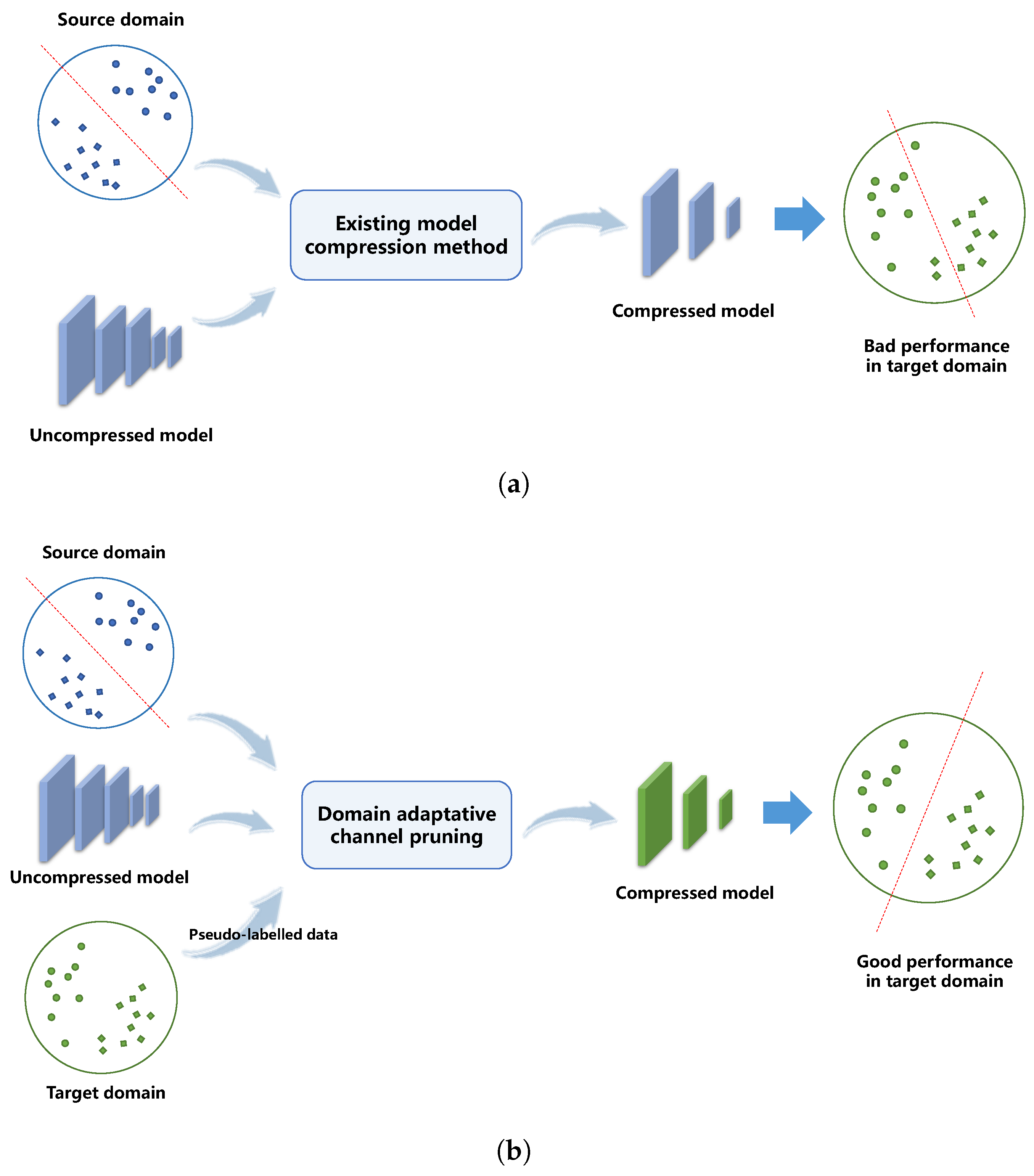
3. Domain Adaptive Channel Pruning

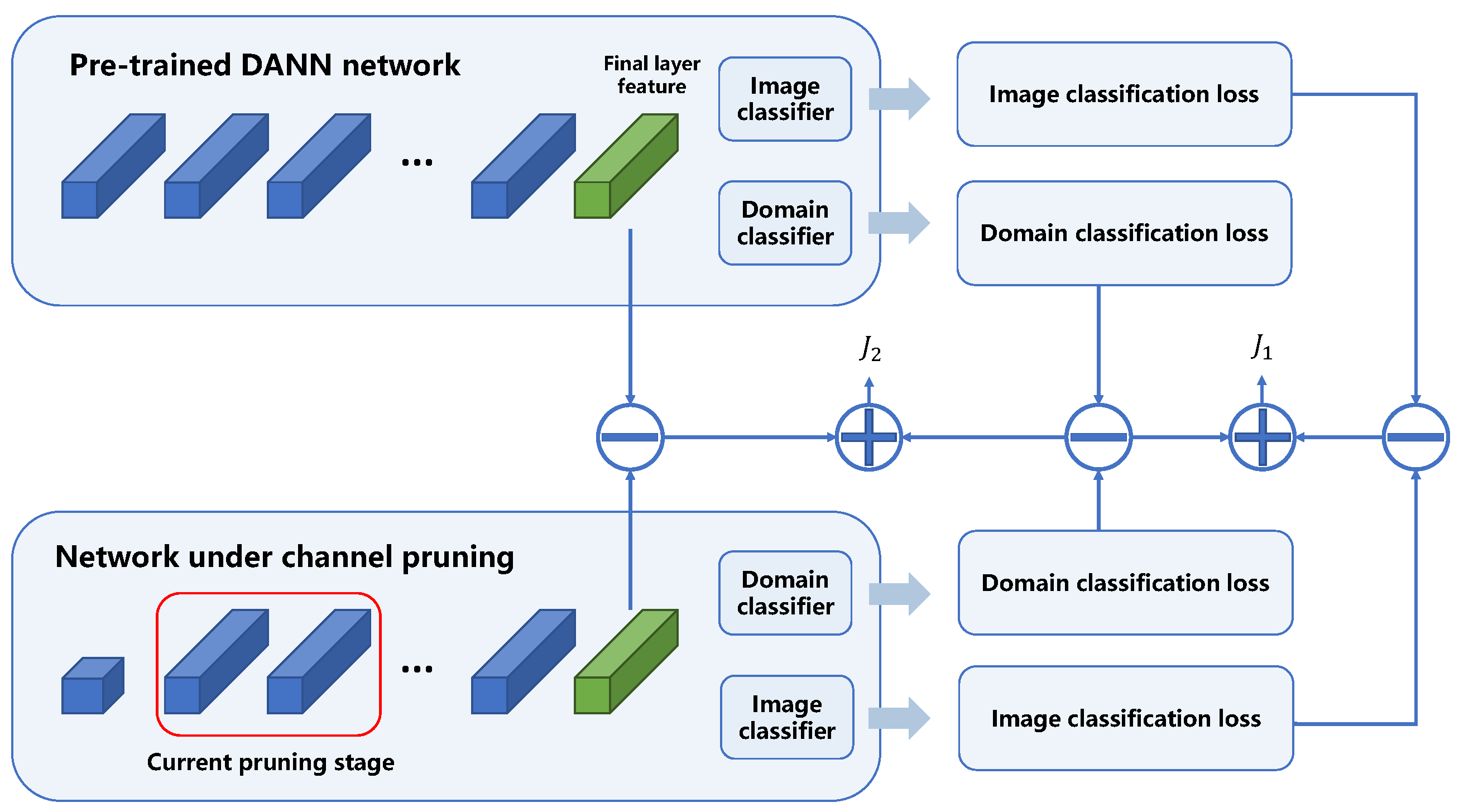
In this section, we first introduce our framework for pruning a model for the unsupervised domain adaptation task. Then, we present the process of pre-training an initial DANN model to reduce the data distribution mismatch between the two domains. After that, we briefly describe the overview of our DACP approach and introduce our DACP method in each layer. We further show how to take the data distribution mismatch issue into consideration during the pruning process. Moreover, we present how to utilize the unlabeled target domain samples by using the pseudo-labels or the features. Finally, we briefly describe how to incorporate other deep transfer learning approaches like Deep Adaptation Networks (DAN) [5] in our DACP approach.

3.1. Framework

Given a deep model pre-trained on ImageNet [42], we use the following three steps to prune the model.

1. Pre-train the deep model. To obtain the initial model, we first train the deep model by using the DANN method in [4]. Training details can be seen in Section 3.2.

2. Channel pruning by DACP. After obtaining the pre-trained DANN model, we first predict the pseudo-labels of samples in the target domain. Then, we use the DACP method described in Section 3.4 to prune the channels in a layer-by-layer fashion.

3. Fine-tuning. After pruning the model, we fine-tune the pruned model by using the DANN method to recover from the accuracy drop and further reduce the data distribution mismatch between different domains.

3.2. Pre-Train the Initial Model Using DANN

In order to reduce the data distribution mismatch between two domains, we first pre-train the initial model by using the DANN [4] approach. The DANN network consists of three parts: the feature extractor F, the image classifier C, and the domain classifier D. The feature extractor F uses CNN (e.g., VGG [43]) as the backbone. The image classifier C consists of fully connected layers to classify the images. Similar to the structure of the image classifier C, the domain classifier D decides whether a sample is from the source or target domain. The DANN method aims to learn the feature extractor that (1) minimizes the image classification error and (2) maximizes the domain classification error. Maximization of the domain classification error increases the difficulty in distinguishing whether the learned features are from the source or target domain. In this way, the learned features are enforced to bridge the domain gap.

3.3. Overview of Our DACP Approach

Given a pre-trained initial DANN model, our goal is to compress this model so as to achieve the best performance on the target domain under a given model compression ratio. We call the pre-trained DANN model as the uncompressed model. And its corresponding model after compression is called the compressed model. Assuming the uncompressed model is trained by a cost (e.g., cross-entropy loss), we aim to keep the cost of the compressed model close to the cost of the uncompressed model.

Figure 2 shows an overview of our DACP approach. Given an uncompressed model, we use this model to predict the pseudo-labels of the samples in the target domain. Then, we will prune the channels of the uncompressed model in a layer-by-layer fashion from shallow layer (closer to the image) to deep layer (closer to the output). We prune the channels in order to minimize (1) the difference of image classification error or (2) the difference of output features at the last convolutional layer, between the uncompressed model and the compressed model, depending on the confidence of predicted pseudo-labels.

3.4. DACP in Each Layer

For better representation, we introduce our DACP approach in each layer in this section.

Formulation. We denote the input feature of layer l by $\mathbf{X}\in {\mathbb{R}}^{c_{in}\times h_{in}\times w_{in}}$ and the output feature of layer l by $\mathbf{Y}\in {\mathbb{R}}^{c_{out}\times h_{out}\times w_{out}}$. The l-th convolutional layer connects the features $\mathbf{X}$ and $\mathbf{Y}$. We denote $\mathbf{W}\in {\mathbb{R}}^{c_{out}\times c_{in}\times h_k\times w_k}$ as the convolutional filters at layer l. The output feature $\mathbf{Y}$ can be calculated as:

$${\mathbf{Y}}_{i,:,:}=\sum _{j=1}^{c_{in}}{\beta }_j{\mathbf{X}}_{j,:,:}\ast {\mathbf{W}}_{i,j,:,:},$$

(1)

where ${\mathbf{X}}_{j,:,:}$ is the j-th channel of the input feature $\mathbf{X}$. ${\mathbf{Y}}_{i,:,:}$ is the i-th channel of the output feature $\mathbf{Y}$. ${\mathbf{W}}_{i,j,:,:}$ is the j-th channel of the i-th convolutional filter $\mathbf{W}$. ∗ is the convolution operation. $\beta \in {\{0,1\}}^{c_{in}}$ is the vector containing a set of binary channel selection indicators ${\beta }_j,j=1,\dots ,c_{in}$. When ${\beta }_j=0$, the j-th channel of the input feature $\mathbf{X}$ will be pruned. We omit the summation over samples, the activation function, and bias term for better representation.

Let us denote ${\mathbf{Y}}^0$ as the output feature at the l-th layer of the uncompressed model. After pruning the channels by setting ${\beta }_j=0$ for several channel indices j, the compressed model will have an output feature $\mathbf{Y}$ at the l-th layer. Let us denote $\mathcal{L}\left(\mathbf{Y}\right)$ as the cost function when the output feature at the l-th layer is $\mathbf{Y}$. The cost function takes two factors into account: image classification error and domain gap. Details of the cost function are given in Section 3.5.

Our DACP method is formulated as minimizing the difference between the output of the cost functions $\mathcal{L}\left({\mathbf{Y}}^0\right)$ and $\mathcal{L}\left(\mathbf{Y}\right)$ as follows:

$$J_1={\left[\mathcal{L}\left(\mathbf{Y}\right)-\mathcal{L}\left({\mathbf{Y}}^0\right)\right]}^2.$$

(2)

By minimizing the objective function $J_1$ defined above, the cost of the compressed model after pruning some channels should be close to the cost of the uncompressed model.

Approximation by Taylor expansion. Exhaustive search of the binary indicators $\beta$ is intractable, as it requires $2^{C_{in}}$ evaluations of $J_1$ to choose the most representative channels. Considering $C_{in}$ is usually several hundreds in VGG [43] or ResNet [44], it is impossible to perform an exhaustive search. To handle this problem, we approximate the cost function by using the first-order Taylor expansion.

For the l-th layer, let us denote $y_{i,m}^0$ and $y_{i,m}$ as the output features of the i-th channel at location m for the uncompressed model and compressed model, respectively. $y_{i,m}^0$ and $y_{i,m}$ belong to the same spatial location m and the i-th channel. $y_{i,m}^0$ is an element in ${\mathbf{Y}}^0$, and $y_{i,m}$ is an element in $\mathbf{Y}$. Since we expect the output of the cost function for $\mathbf{Y}$ and ${\mathbf{Y}}^0$ to be as close as possible, we approximate the cost function $\mathcal{L}\left(\mathbf{Y}\right)$ near ${\mathbf{Y}}^0$ by using the first-order Taylor expansion as follows:

$$\mathcal{L}\left(\mathbf{Y}\right)\approx \mathcal{L}\left({\mathbf{Y}}^0\right)-\sum _{i=1}^{c_{out}}\sum _{m=1}^M\frac{\partial \mathcal{L}}{\partial y_{i,m}}(y_{i,m}^0-y_{i,m}),$$

(3)

where M is the length of the vectorized feature map. Putting the derived results in Equation (3) to Equation (2), the objective function can be rewritten as:

$$\begin{array}{c}\hfill J_1\approx {\left[\sum _{i=1}^{c_{out}}\sum _{m=1}^M\frac{\partial \mathcal{L}}{\partial y_{i,m}}(y_{i,m}^0-y_{i,m})\right]}^2\le M·c_{out}·\sum _{i=1}^{c_{out}}\sum _{m=1}^M{\left[\frac{\partial \mathcal{L}}{\partial y_{i,m}}(y_{i,m}^0-y_{i,m})\right]}^2,\end{array}$$

(4)

where $\frac{\partial \mathcal{L}}{\partial y_{i,m}}$ is the partial derivative of the cost function with respect to $y_{i,m}$. Equation (4) implicates an upper-bound of our objective function $J_1$. This upper-bound can be proved by the power mean inequality. Therefore, we will minimize this upper-bound.

Solution. We define the final objective function as follows:

$$\begin{array}{c}\hfill \underset{\mathit{\beta },\mathbf{W}}{arg\; min}{J}_1=\sum _{i=1}^{c_{out}}{\left[\frac{\partial \mathcal{L}}{\partial y_i}·(y_i^0-y_i)\right]}^2,\mathrm{subject}\mathrm{to}{\parallel \mathit{\beta }\parallel }_0\le B,\end{array}$$

(5)

where $y_i={\sum }_{j=1}^{c_{in}}{\beta }_j{\widehat{\mathbf{X}}}_{j,:,:}\ast {\mathbf{W}}_{i,j,:,:}$, ${\widehat{\mathbf{X}}}_{j,:,:}$ are the input features at the j-th channel used for obtaining the output feature $y_i$ through the filter ${\mathbf{W}}_{i,j,:,:}$. ∗ is the convolutional operation. $\mathit{\beta }$ is the vector containing a set of channel selection indicators ${\beta }_j,j=1,\cdots ,c_{in}$. B is the pre-defined number of remaining channels. We omit the constant term $M·c_{out}$ in Equation (5) because it does not affect the optimization solution. We also omit the spatial location m in Equation (5) for better presentation. The solution for multiple spatial locations can be readily obtained.

Solving the objective function in Equation (5) is NP-hard. Therefore, we relax the $l_0$ to $l_1$ regularization:

$$\begin{array}{c}\hfill \underset{\mathit{\beta },\mathbf{W}}{arg\; min}\sum _{i=1}^{c_{out}}{\left[\frac{\partial \mathcal{L}}{\partial y_i}·(y_i^0-y_i)\right]}^2+{\lambda \parallel \mathit{\beta }\parallel }_1,\mathrm{subject}\mathrm{to}{\parallel \mathit{\beta }\parallel }_0\le B,\end{array}$$

(6)

where $\lambda$ is the coefficient to balance different terms. Following [24,45], we use the same process to solve the optimization problem in Equation (6).

3.5. Choice of the Cost Function

In order to reduce the data distribution mismatch, we choose the cross-entropy loss for both the image classifier and domain classifier as our cost function since the cross-entropy loss is a common loss function designed for classification tasks, which is widely used in many works [2,46]. When the output feature at the l-th layer is $\mathbf{Y}$, let us denote ${\mathcal{L}}_C\left(\mathbf{Y}\right)$ and ${\mathcal{L}}_D\left(\mathbf{Y}\right)$ as the cost (i.e., cross-entropy loss) for the image classifier and the domain classifier, respectively. Our objective function $J_1$ can be written as:

$$J_1={\left[{\mathcal{L}}_C\left(\mathbf{Y}\right)-{\mathcal{L}}_C\left({\mathbf{Y}}^0\right)\right]}^2+\alpha {\left[{\mathcal{L}}_D\left(\mathbf{Y}\right)-{\mathcal{L}}_D\left({\mathbf{Y}}^0\right)\right]}^2,$$

(7)

where $\alpha$ is the coefficient to balance the two differences. By choosing the cross-entropy loss from both the image and the domain classifiers, we minimize the distance from not only the image classification loss, but also the domain classification loss between the compressed model and the initial model. In this way, we take the domain distribution mismatch into consideration.

3.6. Efficient Use of Samples from the Target Domain

Since the samples from the target domain are unlabeled, it is important to use the samples in the target domain effectively. To this end, we propose two strategies to utilize the unlabeled samples from the target domain.

1. Use of pseudo-label. We use the initial DANN model to predict the class labels of unlabeled samples in the target domain and use the predicted class labels as the pseudo-labels. Then, we use the labeled samples from the source domain and the pseudo-labeled samples from the target domain as our training samples to prune the model by using the method described in Section 3.4.

2. Handling pseudo-labeled samples with low confidence. When using the pseudo-labeled data for channel pruning, a key problem is: what if the pseudo-labels of the images are wrong? To solve this problem, we further propose a method to adaptively choose pseudo-labels or output features at the last convolutional layer to guide the channel pruning process. Specifically, the initial DANN model will estimate the probability $\left\{P\right(cls\left)\right|cls=1,\dots ,C\}$ of a target sample belonging to class $cls$. We firstly predict the class of each sample in the target domain by $cl{s}^{ps}={arg\; max}_{cls}P\left(cls\right)$. Then, we use the predicted class $cl{s}^{ps}$ of this target sample as our pseudo-labeled class. We use the predicted probability $P\left(cl{s}^{ps}\right)$ as the confidence of our prediction. For the samples with the confidence higher than a threshold $TH$, we choose the image classification loss ${\mathcal{L}}_C\left(\mathbf{Y}\right)$; for the samples with the confidence lower than $TH$, we choose the sum of squared difference between the output features from the compressed model and the uncompressed model at the last convolutional layer, which is inspired by the knowledge distillation work in [47,48]. The difference is that we use features instead of predicted probability of each class for knowledge distillation. Formally, consider the output feature $\mathbf{Y}$ at the l-th layer; we use $\mathcal{G}\left(\mathbf{Y}\right)$ to represent the output feature at the final convolutional layer in the network. We will minimize the following objective function:

$$J_2=\left|\right|\mathcal{G}\left(\mathbf{Y}\right)-\mathcal{G}\left({\mathbf{Y}}^0\right){\left|\right|}_F^2+\alpha {\left[{\mathcal{L}}_D\left(\mathbf{Y}\right)-{\mathcal{L}}_D\left({\mathbf{Y}}^0\right)\right]}^2,$$

(8)

where $\left|\right|·{\left|\right|}_F$ denotes the Frobenius norm. We minimize the change of the output features at the last convolutional layer by simply replacing $\frac{\partial \mathcal{L}}{\partial y_i}$ in Equation (5) by $\frac{\partial \mathcal{G}}{\partial y_i}$. In this way, our DACP approach can adaptively choose the pseudo-labels by using $J_1$ or the features by using $J_2$ according to the confidence of the pseudo-labels in order to avoid the problem from wrongly predicted pseudo-labels.

3.7. Pruning with DAN

The Deep Adaptation Networks (DAN) method [5] consists of three parts: the feature extractor F, and the image classifiers $C_s$ and $C_t$ for the samples from the source domain and the target domain, respectively. Similar to the DANN method, the DAN approach uses the CNNs as the backbone for feature extractor F. Both of the image classifiers $C_s$ and $C_t$ consist of several fully connected layers. The DAN approach uses the Maximum Mean Discrepancy (MMD) to calculate the data distribution distance between the source domain and the target domain based on the representation after each fully connected layer. The feature extractor in DAN is learned by minimizing (1) the cross-entropy loss from the image classification task for the samples from the source domain and (2) the MMD between the source domain and the target domain. In this case, our DACP approach uses the cross-entropy loss from $C_s$ and the data distribution distance to guide the pruning process. Formally, let us denote the output feature $\mathbf{Y}$ at the l-th layer. We use ${\left[\mathcal{H}\left(\mathbf{Y}\right)-\mathcal{H}\left({\mathbf{Y}}^0\right)\right]}^2$ to represent the data distribution distance of the representations after the fully connected layers. We minimize the following objective function:

$$J_3={\left[{\mathcal{L}}_C\left(\mathbf{Y}\right)-{\mathcal{L}}_C\left({\mathbf{Y}}^0\right)\right]}^2+\nu {\left[\mathcal{H}\left(\mathbf{Y}\right)-\mathcal{H}\left({\mathbf{Y}}^0\right)\right]}^2,$$

(9)

where $\nu$ is the coefficient to balance the two differences. In this way, our DACP approach can be readily used to prune the channels for the DAN method.

4. Experiment

In this section, we follow some related work [2,24,28] to take three popular models, VGG16 [43], AlexNet [49], and ResNet-50 [44], as the backbone in the DANN method to evaluate our DACP approach under the unsupervised domain adaptation setting on two datasets specifically designed for domain adaptation tasks: Office-31 [50] and ImageCLEF-DA [51]. As our baseline methods DANN [4] and CP [24] use VGG16 [43], AlexNet [49], and ResNet50 [44] as the backbone networks, we follow our baseline methods to also choose these three backbone networks in our experiments for fair comparison. Moreover, we investigate the components of our method in details. We further take AlexNet as the backbone in the DAN method to evaluate our approach under the unsupervised domain adaptation setting on the ImageCLEF-DA dataset.

4.1. Implementation Details

We pre-train our initial model by using the DANN method [4] with the stochastic gradient descent (SGD) optimizer. Similar to [5], we use the initial learning rate of $0.0005$ and gradually decrease the learning rate by using the INV function as other unsupervised domain adaptation methods [2,4]. Considering the trade-off between model convergence results and running speed, we set the batch size and momentum as 32 and 0.9, respectively. In this way, we firstly reduce the data distribution mismatch between the two domains and obtain a good initial model before channel pruning. When choosing the pseudo-labels to guide the pruning process, we conduct experiments using different $TH$ values and find that $TH=0.3$ achieves the best result. Therefore, we empirically set $TH=0.3$ by default. The coefficient to balance the image classification loss and the domain classification loss $\alpha$ is set to 0.1. During the fine-tuning stage, we use the same INV function to decrease the learning rate as the pre-training stage by using the initial learning rate varying from $0.0001$ to $0.000001$ to fine-tune the compressed models. Other hyper-parameters are the same as those in the pre-training stage.

In order to demonstrate the effectiveness of our DACP method, several baseline methods are listed below for comparison.

1. VGG16 (resp. AlexNet, ResNet50): We first pre-train the VGG16 (resp. AlexNet, ResNet50) model by using the ImageNet [42] dataset and fine-tune the pre-trained model based on the labeled source domain data without using the DANN method [4]. The model VGG16 (resp. AlexNet, ResNet50) is not compressed.

2. DANN: We first pre-train the VGG16 (resp. AlexNet, ResNet50) model by using the ImageNet dataset and fine-tune the pre-trained VGG16 (resp. AlexNet, ResNet50) model by using the DANN approach based on the Office-31 [50] or the ImageCLEF-DA [51] dataset. This model is used as our initial uncompressed model to be pruned.

3. CP [24]: We directly use the method in [24] to prune the initial DANN model by using the labeled samples from the source domain because the source code is publicly available. Then, we fine-tune the compressed model with the DANN approach.

4. DACP: We use our newly proposed DACP approach to prune the uncompressed model by using the labeled samples from the source domain and adaptively choose pseudo-labels or features from the target domain. Then, we fine-tune the pruned model with the DANN approach.

In this section, the compression ratio (CR) refers to the ratio of the floating point operations (FLOPs) between the uncompressed model and the compressed model, which is a commonly used criterion for computational complexity measurement. For all compressed models, we directly report the accuracies after the fine-tuning process.

4.2. Experiments on Office-31

The Office-31 dataset [50] is a benchmark dataset to evaluate the domain adaptation methods for object recognition, which consists of 4110 real images from 31 classes. There are three domains in Office-31: Amazon (A), Webcam (W), and DSLR (D). We follow the original DANN work [4] to use the commonly used evaluation protocol.

Table 1. Accuracies (%) of different channel pruning methods for pruning DANN-VGG16 under 5× compression ratio, DANN-AlexNet under 3× compression ratio, and DANN-ResNet50 under 2× compression ratio on the Office-31 dataset, respectively.

Methods	A→W	W→A	A→D	D→A	D→W	W→D	Avg.
VGG16 [43]	70.0	56.4	74.1	53.5	95.7	99.0	74.8
DANN-VGG16	81.9	64.3	80.9	63.4	97.1	99.6	81.2
CP-VGG16 [24]	75.5	60.7	77.9	58.4	95.5	98.6	77.8
DACP-VGG16	82.0	64.1	80.9	63.0	97.0	99.6	81.1
AlexNet [49]	61.6	49.8	63.8	51.1	95.4	99.0	70.1
DANN-AlexNet	64.9	47.9	70.9	50.8	95.1	97.8	71.2
CP-AlexNet [24]	57.6	45.3	60.4	46.1	91.7	97.0	66.4
DACP-AlexNet	64.4	47.7	70.9	51.3	95.1	97.8	71.2
ResNet50 [44]	68.4	60.7	68.9	62.5	96.7	99.3	76.1
DANN-ResNet50	82.6	64.2	81.1	63.4	97.0	99.4	81.3
CP-ResNet50 [24]	80.6	61.3	79.7	60.1	95.9	98.2	79.3
DACP-ResNet50	83.2	64.1	81.1	64.3	96.6	99.4	81.5

shows the results for compressing DANN-VGG16 (CR = 5×), DANN-AlexNet (CR = 3×), DANN-ResNet50 (CR = 2×) models on the Office-31 dataset. Our DACP approach outperforms the CP method [24] in all the settings. The improvements clearly demonstrate the effectiveness of our DACP approach. Moreover, it is interesting to observe that DANN-VGG16, DANN-AlexNet, DANN-ResNet50 usually outperform the corresponding models VGG16, AlexNet, ResNet50, which are fine-tuned without using the DANN method. The results indicate that it is beneficial to reduce the data distribution mismatch by using the DANN approach before the channel pruning process. We would like to highlight that the compressed model DACP-ResNet50 even surpasses the initial DANN-ResNet50 model in terms of the average accuracy on the Office-31 dataset. One possible explanation is that our DACP-ResNet50 additionally utilizes pseudo-labeled samples from the target domain.

4.3. Experiments on ImageCLEF-DA

We also perform the experiments on another benchmark dataset: ImageCLEF-DA [51]. The ImageCLEF-DA dataset consists of 4 subsets: Caltech-256 (C), ImageNet ILSVRC 2012 (I), Bing (B), and Pascal VOC 2012 (P). Each subset contains 12 classes and each class has 50 images. We follow [51] to report the results on all six settings.

Table 2. Accuracies (%) of different channel pruning methods for pruning DANN-VGG16 under 5× compression ratio, DANN-AlexNet under 3× compression ratio, and DANN-ResNet50 under 2× compression ratio on the ImageCLEF-DA dataset, respectively.

Methods	I→C	C→I	I→P	P→I	C→P	P→C	Avg.
VGG16 [43]	89.7	74.2	71.6	83.2	62.3	87.8	78.1
DANN-VGG16	92.2	81.8	71.9	84.8	70.4	87.3	81.4
CP-VGG16 [24]	82.8	71.2	64.6	77.3	62.9	83.3	73.7
DACP-VGG16	90.7	78.2	70.4	83.5	68.4	87.3	79.8
AlexNet [49]	84.3	71.3	66.2	70.0	59.3	84.5	73.9
DANN-AlexNet	85.8	73.5	66.5	74.5	60.9	85.8	74.5
CP-AlexNet [24]	73.7	64.2	56.2	60.3	53.1	70.3	63.0
DACP-AlexNet	84.7	70.5	61.4	73.0	59.6	83.5	72.1
ResNet50 [44]	91.5	78.0	74.8	83.9	65.5	91.2	80.7
DANN-ResNet50	92.8	85.0	72.1	85.8	73.1	91.0	83.3
CP-ResNet50 [24]	85.3	71.7	62.4	76.2	59.2	80.7	72.6
DACP-ResNet50	92.5	84.0	70.9	85.5	72.4	90.2	82.6

shows the results for compressing DANN-VGG16 (CR = 5×), DANN-AlexNet (CR = 3×), DANN-ResNet50 (CR = 2×) models on the ImageCLEF-DA dataset. Again, our DACP method outperforms the CP method [24] in all the settings. The results further demonstrate the effectiveness of our DACP method.

4.4. Ablation Study

In this section, we take DANN-AlexNet as an example to analyze different aspects of our method for model compression on the ImageCLEF-DA dataset. To study the effect of each component in our method, we perform the experiments under six settings, and the results are reported in

Table 3. Accuracies (%) after pruning the DANN-AlexNet model on the ImageCLEF-DA dataset under a compression ratio of 3× without consideration of: domain gap, pseudo-labels, adaptive choice of pseudo-labels or features.

Methods	I→C	C→I	I→P	P→I	C→P	P→C	Avg.
DACP-AlexNet	84.7	70.5	61.4	73.0	59.6	83.5	72.1
DACP w/o DG	77.0	67.5	58.9	65.5	57.9	74.5	66.9
DACP w/o PL	76.3	65.0	58.9	62.8	53.1	73.3	64.9
DACP w/o AC	82.3	70.0	60.2	71.3	58.4	83.2	70.9

:

(1) DACP without considering the domain gap (DACP w/o DG): we use the difference of the cross-entropy loss from the image classification task ${\mathcal{L}}_C\left(\mathbf{Y}\right)$ as the objective function $J_1$ and remove the domain classification loss in Equation (7). In this case, the domain gap is not considered during channel pruning. In Table 3, the average accuracy drops 5.2%, which shows that it is effective to reduce the domain distribution mismatch in the pruning process.

(2) DACP without considering the pseudo-label (DACP w/o PL): we only use the labeled samples from the source domain in the pruning process. In this case, pseudo-labeled target samples are not used to guide the pruning process. The average accuracy drops 7.2% in this case, which demonstrates that the performance can be significantly improved by using the pseudo-labeled samples in the target domain.

(3) DACP without using adaptive choice of pseudo-labels or features (DACP w/o AC). In this case, we only use the pseudo-labels to guide the channel pruning process but do not use the features even when the confidence of pseudo-label is low. The average accuracy drops 1.2%, which shows the effectiveness of the adaptive choice of pseudo-labels or features.

4.5. Channel Pruning Results for DAN

We further take AlexNet [49] as the backbone network in the Deep Adaptation Networks (DAN) approach [5] as an example to demonstrate that our DACP method can also be used for other unsupervised domain adaptation methods. The coefficient to balance two differences $\nu$ is set to 1.

Table 4. Accuracies (%) after pruning the DAN-AlexNet model on the ImageCLEF-DA dataset under the compression ratio of 3×.

Methods	I→C	C→I	I→P	P→I	C→P	P→C	Avg.
AlexNet [49]	84.3	71.3	66.2	70.0	59.3	84.5	73.9
DAN-AlexNet	85.8	74.7	65.3	78.0	60.9	85.8	75.1
CP-AlexNet [24]	75.0	57.3	55.3	61.2	48.9	68.2	61.0
DACP-AlexNet	83.3	72.7	63.8	76.8	59.4	81.0	72.8

shows the results for compressing DAN-AlexNet (CR = 3×) model on the ImageCLEF-DA dataset. Our DACP approach outperforms the CP method in all the settings, which again demonstrates the effectiveness of our DACP approach.

5. Conclusions

In this work, we have proposed the specifically designed Domain Adaptive Channel Pruning (DACP) approach to compress CNNs under the unsupervised domain adaptation setting. Our method minimizes a cost that considers the considerable data distribution mismatch between different domains but without frequently requiring the time-consuming fine-tuning process. We have also proposed an effective approach to utilize the unlabeled samples in the target domain. Comprehensive experiments on two benchmark datasets demonstrate the effectiveness of our newly proposed DACP approach for the unsupervised domain adaptation task.

However, our DACP approach also has some weaknesses and limitations. We only use the first-order Taylor expansion, which may lose second-order information and cause inaccurate approximation compared with other pruning methods. Our hyper-parameter settings such as the pseudo-label confidence threshold $TH$ may be sub-optimal; we hope that future research may solve this problem by setting learnable parameters. Moreover, our future direction also includes how to better utilize unlabeled data and extend DACP to unstructured pruning for better performance.

References

1. Csurka, G. Domain Adaptation for Visual Applications: A Comprehensive Survey. arXiv 2017, arXiv:1702.05374. [Google Scholar]
2. Yu, C.; Wang, J.; Chen, Y.; Wu, Z. Accelerating Deep Unsupervised Domain Adaptation with Transfer Channel Pruning. arXiv 2019, arXiv:1904.02654. [Google Scholar]
3. Ro, Y.; Choi, J.Y. Autolr: Layer-wise pruning and auto-tuning of learning rates in fine-tuning of deep networks. In Proceedings of the AAAI Conference on Artificial Intelligence, Online, 2–9 February 2021; pp. 2486–2494. [Google Scholar]
4. Ganin, Y.; Ustinova, E.; Ajakan, H.; Germain, P.; Larochelle, H.; Laviolette, F.; Marchand, M.; Lempitsky, V. Domain-adversarial training of neural networks. J. Mach. Learn. Res. 2016, 17, 1–35. [Google Scholar]
5. Long, M.; Cao, Y.; Wang, J.; Jordan, M. Learning transferable features with deep adaptation networks. In Proceedings of the ICML, Lille, France, 6–11 July 2015; pp. 97–105. [Google Scholar]
6. Long, M.; Zhu, H.; Wang, J.; Jordan, M.I. Unsupervised domain adaptation with residual transfer networks. In Proceedings of the NIPS, Barcelona, Spain, 5–10 December 2016; pp. 136–144. [Google Scholar]
7. Sun, B.; Saenko, K. Deep coral: Correlation alignment for deep domain adaptation. In Proceedings of the ECCV, Amsterdam, The Netherlands, 11–14 October 2016; pp. 443–450. [Google Scholar]
8. Tzeng, E.; Hoffman, J.; Zhang, N.; Saenko, K.; Darrell, T. Deep domain confusion: Maximizing for domain invariance. arXiv 2014, arXiv:1412.3474. [Google Scholar]
9. Bousmalis, K.; Silberman, N.; Dohan, D.; Erhan, D.; Krishnan, D. Unsupervised Pixel-Level Domain Adaptation With Generative Adversarial Networks. In Proceedings of the CVPR, Honolulu, HI, USA, 21–26 July 2017; pp. 3722–3731. [Google Scholar]
10. Bousmalis, K.; Trigeorgis, G.; Silberman, N.; Krishnan, D.; Erhan, D. Domain separation networks. In Proceedings of the NIPS, Barcelona, Spain, 5–10 December 2016; pp. 343–351. [Google Scholar]
11. Ganin, Y.; Lempitsky, V. Unsupervised domain adaptation by backpropagation. In Proceedings of the ICML, Lille, France, 6–11 July 2015; pp. 1180–1189. [Google Scholar]
12. Liu, M.Y.; Tuzel, O. Coupled generative adversarial networks. In Proceedings of the NIPS, Barcelona, Spain, 5–10 December 2016; pp. 469–477. [Google Scholar]
13. Tzeng, E.; Hoffman, J.; Saenko, K.; Darrell, T. Adversarial Discriminative Domain Adaptation. In Proceedings of the CVPR, Honolulu, HI, USA, 21–26 July 2017; pp. 2962–2971. [Google Scholar]
14. Zhang, W.; Ouyang, W.; Li, W.; Xu, D. Collaborative and Adversarial Network for Unsupervised domain adaptation. In Proceedings of the CVPR, Salt Lake City, UT, USA, 18–23 June 2018; pp. 3801–3809. [Google Scholar]
15. Mei, Z.; Ye, P.; Ye, H.; Li, B.; Guo, J.; Chen, T.; Ouyang, W. Automatic Loss Function Search for Adversarial Unsupervised Domain Adaptation. IEEE Trans. Circuits Syst. Video Technol. 2023, 33, 5868–5881. [Google Scholar] [CrossRef]
16. Rastegari, M.; Ordonez, V.; Redmon, J.; Farhadi, A. Xnor-net: Imagenet classification using binary convolutional neural networks. In Proceedings of the ECCV, Amsterdam, The Netherlands, 11–14 October 2016; pp. 525–542. [Google Scholar]
17. Gong, Y.; Liu, L.; Yang, M.; Bourdev, L. Compressing deep convolutional networks using vector quantization. arXiv 2014, arXiv:1412.6115. [Google Scholar]
18. Jaderberg, M.; Vedaldi, A.; Zisserman, A. Speeding up Convolutional Neural Networks with Low Rank Expansions. In Proceedings of the BMVC, Nottingham, UK, 1–5 September 2014. [Google Scholar]
19. Kim, Y.D.; Park, E.; Yoo, S.; Choi, T.; Yang, L.; Shin, D. Compression of deep convolutional neural networks for fast and low power mobile applications. arXiv 2015, arXiv:1511.06530. [Google Scholar]
20. Lebedev, V.; Ganin, Y.; Rakhuba, M.; Oseledets, I.; Lempitsky, V. Speeding-up convolutional neural networks using fine-tuned cp-decomposition. arXiv 2014, arXiv:1412.6553. [Google Scholar]
21. Xue, J.; Li, J.; Gong, Y. Restructuring of deep neural network acoustic models with singular value decomposition. In Proceedings of the Interspeech, Lyon, France, 25–29 August 2013. [Google Scholar]
22. Howard, A.G.; Zhu, M.; Chen, B.; Kalenichenko, D.; Wang, W.; Weyand, T.; Andreetto, M.; Adam, H. Mobilenets: Efficient convolutional neural networks for mobile vision applications. arXiv 2017, arXiv:1704.04861. [Google Scholar]
23. Zhang, X.; Zhou, X.; Lin, M.; Sun, J. ShuffleNet: An Extremely Efficient Convolutional Neural Network for Mobile Devices. In Proceedings of the CVPR, Salt Lake City, UT, USA, 18–23 June 2018. [Google Scholar]
24. He, Y.; Zhang, X.; Sun, J. Channel Pruning for Accelerating Very Deep Neural Networks. In Proceedings of the ICCV, Venice, Italy, 22–29 October 2017; pp. 1398–1406. [Google Scholar]
25. Hu, H.; Peng, R.; Tai, Y.W.; Tang, C.K. Network trimming: A data-driven neuron pruning approach towards efficient deep architectures. arXiv 2016, arXiv:1607.03250. [Google Scholar]
26. Li, H.; Kadav, A.; Durdanovic, I.; Samet, H.; Graf, H.P. Pruning filters for efficient convnets. In Proceedings of the ICLR, San Juan, Puerto Rico, 2–4 May 2016. [Google Scholar]
27. Luo, J.H.; Wu, J.; Lin, W. ThiNet: A Filter Level Pruning Method for Deep Neural Network Compression. In Proceedings of the ICCV, Venice, Italy, 22–29 October 2017; pp. 5068–5076. [Google Scholar]
28. Molchanov, P.; Tyree, S.; Karras, T.; Aila, T.; Kautz, J. Pruning convolutional neural networks for resource efficient inference. In Proceedings of the ICLR, Toulon, France, 24–26 April 2017. [Google Scholar]
29. Guo, J.; Liu, J.; Xu, D. JointPruning: Pruning Networks Along Multiple Dimensions for Efficient Point Cloud Processing. IEEE Trans. Circuits Syst. Video Technol. 2022, 21, 3659–3672. [Google Scholar] [CrossRef]
30. Liu, J.; Guo, J.; Xu, D. APSNet: Toward adaptive point sampling for efficient 3D action recognition. IEEE Trans. Image Process. 2023, 31, 5287–5302. [Google Scholar] [CrossRef] [PubMed]
31. Masana, M.; van de Weijer, J.; Herranz, L.; Bagdanov, A.D.; Alvarez, J.M. Domain-adaptive deep network compression. In Proceedings of the ICCV, Venice, Italy, 22–29 October 2017; pp. 4289–4297. [Google Scholar]
32. Wu, C.; Wen, W.; Afzal, T.; Zhang, Y.; Chen, Y. A compact DNN: Approaching googlenet-level accuracy of classification and domain adaptation. In Proceedings of the CVPR, Honolulu, HI, USA, 21–26 July 2017; pp. 5668–5677. [Google Scholar]
33. Zhong, Y.; Li, V.; Okada, R.; Maki, A. Target Aware Network Adaptation for Efficient Representation Learning. In Proceedings of the ECCV Workshops, Munich, Germany, 8–14 September 2018; pp. 450–467. [Google Scholar]
34. Guo, J.; Xu, D.; Lu, G. CBANet: Toward Complexity and Bitrate Adaptive Deep Image Compression Using a Single Network. IEEE Trans. Image Process. 2023, 32, 2049–2062. [Google Scholar] [CrossRef]
35. Liu, Z.; Li, J.; Shen, Z.; Huang, G.; Yan, S.; Zhang, C. Learning efficient convolutional networks through network slimming. In Proceedings of the CVPR, Honolulu, HI, USA, 21–26 July 2017; pp. 2736–2744. [Google Scholar]
36. Guo, J.; Zhang, W.; Ouyang, W.; Xu, D. Model Compression Using Progressive Channel Pruning. IEEE Trans. Circuits Syst. Video Technol. 2021, 31, 1114–1124. [Google Scholar] [CrossRef]
37. Wen, W.; Wu, C.; Wang, Y.; Chen, Y.; Li, H. Learning structured sparsity in deep neural networks. In Proceedings of the NIPS, Barcelona, Spain, 5–10 December 2016; pp. 2074–2082. [Google Scholar]
38. Guo, J.; Ouyang, W.; Xu, D. Multi-Dimensional Pruning: A Unified Framework for Model Compression. In Proceedings of the IEEE/CVF Conference on Computer Vision and Pattern Recognition (CVPR), Virtual, 14–19 June 2020. [Google Scholar]
39. Zhuang, Z.; Tan, M.; Zhuang, B.; Liu, J.; Guo, Y.; Wu, Q.; Huang, J.; Zhu, J. Discrimination-aware channel pruning for deep neural networks. In Proceedings of the NIPS, Montreal, QC, Canada, 3–8 December 2018; pp. 883–894. [Google Scholar]
40. Guo, J.; Xu, D.; Ouyang, W. Multidimensional Pruning and Its Extension: A Unified Framework for Model Compression. IEEE Trans. Neural Netw. Learn. Syst. 2023, 1–15. [Google Scholar] [CrossRef] [PubMed]
41. Rotman, G.; Feder, A.; Reichart, R. Model Compression for Domain Adaptation through Causal Effect Estimation. arXiv 2021, arXiv:2101.07086. [Google Scholar] [CrossRef]
42. Russakovsky, O.; Deng, J.; Su, H.; Krause, J.; Satheesh, S.; Ma, S.; Huang, Z.; Karpathy, A.; Khosla, A.; Bernstein, M.; et al. Imagenet large scale visual recognition challenge. Int. J. Comput. Vis. 2015, 115, 211–252. [Google Scholar] [CrossRef]
43. Simonyan, K.; Zisserman, A. Very deep convolutional networks for large-scale image recognition. arXiv 2014, arXiv:1409.1556v6. [Google Scholar]
44. He, K.; Zhang, X.; Ren, S.; Sun, J. Deep residual learning for image recognition. In Proceedings of the CVPR, Las Vegas, NV, USA, 27–30 June 2016; pp. 770–778. [Google Scholar]
45. Guo, J.; Ouyang, W.; Xu, D. Channel Pruning Guided by Classification Loss and Feature Importance. In Proceedings of the AAAI Conference on Artificial Intelligence, New York, NY, USA, 7–12 February 2020. [Google Scholar]
46. Kumar, A.; Sattigeri, P.; Wadhawan, K.; Karlinsky, L.; Feris, R.; Freeman, W.T.; Wornell, G. Co-regularized Alignment for Unsupervised Domain Adaptation. arXiv 2018, arXiv:1811.05443. [Google Scholar]
47. Hinton, G.; Vinyals, O.; Dean, J. Distilling the knowledge in a neural network. arXiv 2015, arXiv:1503.02531. [Google Scholar]
48. Guo, J.; Liu, J.; Wang, Z.; Ma, Y.; Gong, R.; Xu, K.; Liu, X. Adaptive Contrastive Knowledge Distillation for BERT Compression. In Proceedings of the Findings of the Association for Computational Linguistics: ACL, Toronto, ON, Canada, 9–14 July 2023; pp. 8941–8953. [Google Scholar]
49. Krizhevsky, A.; Sutskever, I.; Hinton, G.E. Imagenet classification with deep convolutional neural networks. In Proceedings of the NIPS, Lake Tahoe, NV, USA, 3–8 December 2012; pp. 1097–1105. [Google Scholar]
50. Saenko, K.; Kulis, B.; Fritz, M.; Darrell, T. Adapting visual category models to new domains. In Proceedings of the ECCV, Crete, Greece, 5–11 September 2010; pp. 213–226. [Google Scholar]
51. Long, M.; Zhu, H.; Wang, J.; Jordan, M.I. Deep transfer learning with joint adaptation networks. PMLR 2017, 70, 2208–2217. [Google Scholar]
Figure 1. Difference between our DACP approach and the existing model compression methods. (a) Existing model compression method under the setting of domain adaptation, and (b) our DACP approach under the setting of domain adaptation.
Electronics 13 00887 g001
Figure 2. The overview of our DACP approach. For labeled samples from the source domain and pseudo-labeled samples with high confidence from the target domain, we aim to minimize J 1 (more details in Section 3.4). For pseudo-labeled samples with low confidence from the target domain, we minimize J 2 (more details in Section 3.6).
Electronics 13 00887 g002