Abstract
Non-negative matrix factorization (NMF) has been used in various applications, including local damage detection in rotating machines. Recent studies highlight the limitations of diagnostic techniques in the presence of non-Gaussian noise. The authors examine the impact of non-Gaussianity levels on the extraction of the signal of interest (SOI). The simple additive model of the signal is proposed: SOI and non-Gaussian noise. As a model of the random component, i.e., noise, a heavy-tailed -stable distribution with two important parameters ( and ) was proposed. If SOI is masked by noise (controlled by ), the influence of non-Gaussianity level (controlled by ) is more critical. We performed an empirical analysis of how these parameters affect SOI extraction effectiveness using NMF. Finally, we applied two NMF algorithms to several (both vibration and acoustic) signals from a machine with faulty bearings at different levels of non-Gaussian disturbances and the obtained results align with the simulations. The main conclusion of this study is that NMF is a very powerful tool for analyzing non-Gaussian data and can provide satisfactory results in a wide range of a non-Gaussian noise levels.
1. Introduction
Methods based on time-frequency representation are frequently used for local damage detection in rotating/recuperating machines [1,2]. The reason for this is simple: such signals are non-stationary, and it is reasonable to track the variation in spectral content over time. However, the spectral structure is usually complicated, and some prefiltering is needed for deeper analysis. There is a group of methods based on the selection of the informative frequency band (IFB), which allows us to determine the frequency band corresponding to the damage. Next, by filtering the raw data, the fault can be easily detected using demodulation and envelope spectrum analysis [3]. One of the most popular directions for signal preprocessing is to estimate data driven selectors, which are used as filter characteristics. The most popular approach is based on spectral kurtosis [4,5]. The filter is obtained by calculating the kurtosis value for each of the subsequent frequency bins in the spectrogram.
Over the years, plenty of variations and extensions of this method have appeared. These methods simply replace the kurtosis and use other statistics as selectors, for example, conditional variance [6] Jarque–Bera, Kolmogorov–Smirnov, Cramer–von Mises, Anderson–Darling, and many others [7]. There are also other methods that are based on a discrete division of the frequency spectrum and data representation in the form of a graphical map. The most popular of them is the Kurtogram proposed by Antoni [8]. It is based on the idea of analyzing the kurtosis of the signal within different frequency bands. In the Kurtogram extensions, the kurtosis is also replaced by other statistics. The infogram [9] is based on the measure of the negentropy of the squared envelope and the squared envelope spectrum. Zhao et al. proposed a harsogram [10] using the harmonic significant index (HSI). In [11], Miao et al. introduce a sparsity index, which is also called the Gini index, as a different approach to selecting the resonance band. The paper [12] is based on the spectral smoothness index, defined as the ratio of the geometric mean to the arithmetic mean of the moduli of the Gabor wavelet coefficient. The autogram is constructed using the autocorrelation of the squared envelope spectrum [13]. TIEgram, which was proposed by Wang et al., is based on an EES analysis as an alternative method for spectrum division [14]. DTMSgram performs noise reduction in the time and frequency domain to improve informative frequency band selection [15]. The SCCPgram [16] is based on optimization of the cyclic periodic index to reveal fault components in vibration signals, providing an effective and improved envelope spectrum. Another method uses the parameters obtained from fitted statistical distributions to assess the level of information in a specific frequency range. For example, the alphagram technique relies on the -stable distribution [17]. The improved envelope spectrum through the feature optimization-gram, called IESFOgram [18,19,20], has been proposed to determine an optimal informative frequency band. The diagnostic feature indicator was used to assess the richness of information related to bearing faults within a specific frequency range.
Unfortunately, in real life, the problem of detecting damage is much more complicated. For example, in a crusher or vibrating screen, falling rocks cause an additional high-amplitude impulsive component in addition to the cyclic impulses from the fault [6,21]. In this case, the most basic and popular selector, such as kurtosis, failed because it focuses on the strongest (random here) impulsive component. However, since cyclic and random impulses do not overlap spectrally (or are partially overlapped), some of the methods mentioned still work [6,9,11].
However, what happens when the random impulses are wideband or completely overlap the IFB? Due to the construction of selectors and their extensions, it will be almost impossible to extract the damage signature without the random component based only on the frequency domain. The researchers also take into account a cyclostationary approach. One of the most popular algorithms is the Cyclic Spectral Coherence (CSC) [22]. It is a bi-frequency map that indicates cyclic modulations in the data. Moreover, one can also find papers that proposed other two-dimensional methods for analyzing cyclostationary signals, also with a non-Gaussian distribution [23]. The generalized spectral coherence [24], fractional lower-order cyclic correlation analysis [25,26,27,28,29], and cyclic correntropy and its spectral versions [30,31,32] are particularly noteworthy.
One of the most basic—but still powerful—and intuitive methods for the presentation of a time–frequency behavior in data is the short-time Fourier transform (STFT). Even if it has some problems with poor resolution, it has strong physical interpretation and interesting properties—energy in the time–frequency plane is always non-negative. It allows us to apply a family of algorithms for non-negative matrix factorization (NMF). This approach has gained popularity in the detection of local damage based on vibration data in recent years [33,34,35,36,37,38,39].
Numerous papers address the issue of non-Gaussianity in background noise. In this context, Wei et al. [40] proposed the improved adaptive multipoint optimal minimum entropy deconvolution (IAMOMED) method, specifically designed to handle random impulsive noise adaptive minimum entropy deconvolution. The method employs an envelope autocorrelation function and particle swarm optimization to enhance fault detection capabilities in the presence of strong random impulsive noise. Zhao et al. [41] propose a fault diagnosis method for rolling element bearings based on a cyclic correntropy (CCE) function and its spectrum. Another interesting method that uses the testing parameters of the fitter -stable distribution is proposed in [17].
This study presents an approach that demonstrates the effectiveness of a tool such as NMF for vibration and acoustic data analysis. The authors take into consideration two NMF algorithms: a multiplicative one for minimizing the Euclidean objective (Standard NMF) [42] and a generalized version of the hierarchical alternating least square algorithm (-HALS) for minimizing the Beta-divergence [43,44], and study the influence of two parameters of the -stable noise on NMF effectiveness. By changing the parameters of the probability distribution (stability index and scale parameter ), the authors modify the level of non-Gaussianity and the noise intensity. To evaluate both NMF models, 25 levels of the parameter and four levels of were taken into account. The main goal of this study is to demonstrate how the effectiveness of the NMF algorithms changes with these two parameters, and to determine the level at which the algorithms no longer return reliable results with a satisfactory probability. This information can be used as a warning to users in practical applications.
The rest of this study is organized as follows. Section 2 provides the main concepts of the tools used. The results of the simulations and the real data analysis are presented next in Section 3. After that, the results obtained are discussed in Section 4. Finally, the conclusions are formulated in Section 5.
2. Methodology
Notation: Matrices, vectors, and scalars are denoted by boldface uppercase letters (e.g., ), lowercase boldface letters (e.g., ), and unbolded letters (e.g., x), respectively. The -th element of matrix is equivalently denoted by or .
In this paper, the authors use a simple additive model of the vibration signal. The first of the components (described in Section 2.1) is the impulsive signal that corresponds to the fault in the real-life signal. The second component is the non-Gaussian noise. In this particular case, it is the -stable noise described in detail in Section 2.2.
2.1. Signal of Interests
The signal of interest (SOI) is composed of a series of individual impulses. They are located in time with a given period T, where corresponds to the fault frequency in the real signal.
The single impulse (see Figure 1) is specified as a decaying harmonic oscillation and can be represented as follows:
where A is the amplitude, is the center frequency, is the decay coefficient of the exponential function (denoted e), and t is the time. The center frequency is related to the structural resonance in the machine. For simplicity, we neglected jitter effects.
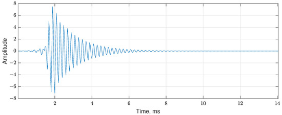
Figure 1.
Example of the single impulse.
2.2. -Stable Component
To simulate the non-Gaussian behavior occurring in the vibration signal, the authors used the -stable distribution, which is characterized by four parameters (denoted as ). In the literature, a few equivalent definitions of this distribution can be found [45,46,47].
The random variable X is called -stable if its characteristic function is given by:
where is the stability index, is the skewness, is the scale parameter, is the shift parameter, and j is the imaginary operator. It is important that is not equal to the standard deviation. For , the -stable distribution is reduced to the Gaussian one with mean and variance equal to ; therefore, the effectiveness of tested NMF models is also verified for the case of Gaussian noise. In this study, the simplified symmetric version of the -stable distribution is used (denoted )—parameters and are equal to 0. The remaining two parameters and have a significant impact on the results obtained, so the authors performed the analysis for 25 levels of the stability index and four levels of the scale parameter. The -stable component is simulated according to the procedure presented in [48].
2.3. Spectrogram
The STFT is calculated for each analyzed signal. For one-dimensional discrete data s, the STFT is defined as [49]:
where is the frequency bin, is the time point, K is the number of the windows in time domain according to the window size and length of the signal, is the shift window, is the input signal, L is its length, n is the iterator over the samples within the window, and j is the imaginary operator.
In our study, the spectrogram (denoted by Y) is defined as an absolute value of STFT:
2.4. Non-Negative Matrix Factorization
NMF is a powerful feature extraction method, well-known in various areas of research, including multivariate analysis. This method assumes that matrix Y is factorized into two low-rank matrices W and H, and all these three matrices have non-negative entries. For our study, we selected the following computational algorithms for NMF:
- Standard multiplicative update rules (Standard NMF) for minimizing the Euclidean objective (described in Section 2.4.1);
- Generalized hierarchical alternating least squares (-HALS) for minimizing the -divergence (described in the Section 2.4.2).
The fundamental NMF model can be expressed in the following form [42,43,44,50]:
where , defined in Equation (4), is the matrix of the non-negative input spectrogram, is the unknown base matrix with non-negative vectors , is the unknown encoding matrix with non-negative components , , where R is the NMF rank, T is the transposition operator, and is the matrix that corresponds to residual errors or noise. For simplicity, the authors also use the notation , which allows us to use only column vectors.
2.4.1. Standard NMF
To find non-negative low-rank approximations to input noisy matrix Y, the cost function should be tailored to the data distribution. Lee and Seung [50] proposed two options for the cost function, namely: Euclidean distance and generalized Kullback–Leibler (KL) divergence. The square Euclidean distance takes the form:
It is a convex function, but only with respect to one set of arguments, that is, the base (W) or the encoding matrix (H) but not jointly. This is a reason why finding the global minima is an NP-hard problem. However, many optimization techniques can find a good approximation to this problem.
The metric (6) is non-increasing under the update rules:
where ⊗ denotes the elementwise multiplication, and ⊘ denotes elementwise division [50]. Both matrices W and H are usually updated using an alternating optimization scheme. Normalizing matrices W and H results in the energy of the clusters remaining constant. In principle, the normalization is performed by the columns of matrix W, [42]:
where
Similarly to , the normalization of can be performed by applying the scaling to its rows:
where
and is the r-th row vector of for .
2.4.2. -HALS NMF
The hierarchical nature of the algorithm is that it uses a set of local cost functions and minimizes them successively (one by one) [43,44]. Unlike the algorithm described in Section 2.4.1, the local cost function is based on the -divergence (denoted ) between two non-negative sequences. It can be defined as follows:
where , the operator is performed element-wise, , and for .
The learning rules are obtained by calculating the gradients of (12) with respect to elements and . In consequence, the simple HALS update rules are obtained by searching for stationary points. Thus, the update rules for the HALS with the -divergence take the form:
where is an appropriately chosen convex function, and all non-linear operations are performed element-wise.
2.5. Component Reconstruction
Estimated base and encoding vectors of respective matrices W and H are used to construct R rank-1 spectrograms—each created by multiplying one base vector and the corresponding encoding vector. Since the aim is to recover the time series of each component and evaluate the results, the complete complex form representing the STFT needs to be reconstructed. This happens because the built-in Matlab function, used by the authors, takes a complex matrix as input. The aim is to find a complete complex form of STFT that describes the signal represented by the non-negative matrix obtained from the NMF model. To address this problem, the authors used the Griffin–Lim algorithm for phase estimation [51]. Finally, the signals (one signal for one NMF feature) in the time domain are reconstructed from the obtained matrices using the inverse STFT (iSTFT) procedure, which is calculated by the weighted overlap-added algorithm (WOLA) [52].
2.6. Envelope Spectrum
The diagnostic signal amplitude demodulation procedure assumes that the modulating signal carries information about the fault. This signal processing technique for local damage detection is one of the simplest and most popular. The idea of demodulation is to choose an appropriate frequency band, perform bandpass filtering on that band, and then use the Hilbert transform (HT) to determine the envelope signal, the spectrum of which is finally analyzed. In the presented case, the general idea is the same; however, the signals that the authors take for analysis come from the reconstructed components (described in detail in Section 2.5).
First, the envelope of the reconstructed signal is calculated. It can be defined as an absolute value of the analytical signal:
where is the Hilbert transform of the real-valued signal . The algorithm used to approximate the analytical signal was introduced in [53]. It calculates the fast Fourier transform (FFT) of an input sequence, then the FFT coefficients that correspond to negative frequencies are replaced and, in the last step, the inverse FFT of the result is calculated.
Then, the Fourier transform (FT) is applied to the analytical signal defined in Equation (14):
2.7. Envelope Spectrum Based Indicator (ENVSI)
Periodic impulses in the time domain associated with the fault are represented by a family of harmonic components corresponding to the fault frequency in the envelope spectrum. The more evident modulation is observed over time, the higher the amplitude of harmonics. All results obtained by both NMF models must be verified by the same indicator; thus, the authors proposed the ENVSI measure [6]. This simple indicator can be interpreted as a measure of energy. Consider the squared normalized amplitudes of the informative signal in relation to the squared normalized envelope spectrum in the considered frequency range. It can be defined as:
where are normalized amplitudes of the information signal, is the squared normalized envelope spectrum, is the number of harmonics to analyze, and is the number of frequency bins used to calculate the total energy.
ENVSI is applied to the reconstructed time series of each NMF class to calculate the efficiency of the analyzed algorithms.
3. Results
3.1. Simulations
In this Section, the results for simulated data are presented. First, the components are simulated separately and added together. For the purpose of the simulation, the sampling frequency is = 25,000 Hz and the duration is 2 s (50,000 samples).
- Signal of interest (SOI) was generated as described in Section 2.1 with the same parameters for each scenario: amplitude , center frequency kHz, decay coefficient , and the period between the impulses: s, which can translate into the fault frequency equal to 12 Hz.
- —stable noise was generated as described in Section 2.2. The vibration signal in real life is symmetric and centered around zero; hence, and are equal to zero, respectively. Parameter was defined at 25 levels. It decreases from 2 to 1.8 with a resolution of 0.1, and from 1.75 to 1.6 with a resolution of 0.5. Additionally, four values of parameter were considered, namely: 0.3, 0.7, 1, and 1.3.
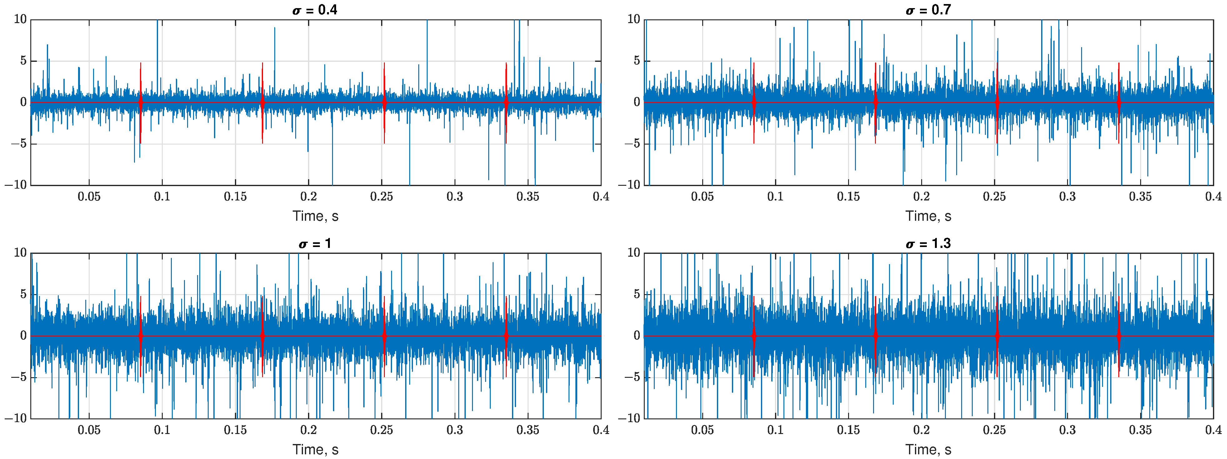
The scale parameter affects the signal-to-noise ratio (SNR), i.e., it controls the level of noise and may cause the SOI impulses to be completely hidden in the noise. When is equal to , the SOI is clearly visible over the noise, and while the scale parameter increases, the visibility of the SOI decreases. For the highest analyzed value, , the SOI is fully masked by the noise in the time series. In Figure 2, one can see how a change in the scale value (0.4, 0.7, 1, and 1.3, respectively) can influence the SNR or, in other words, the visibility of the cyclic impulses (marked red) in the observed signal.
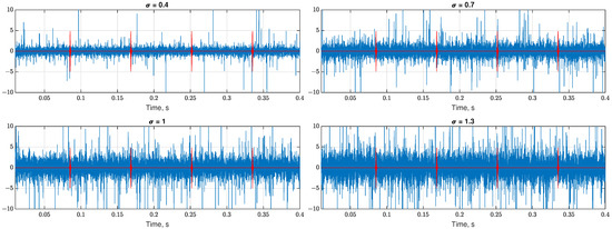
Figure 2.
Cyclic impulses (marked red) hidden in -stable noise, , scale parameters: 0.4, 0.7, 1, and 1.3, respectively.
Due to the resolution of (25 levels) and (4 levels), the authors have obtained 100 time series for each case. This procedure was repeated 100 times, giving 10,000 time series as the tested data set.
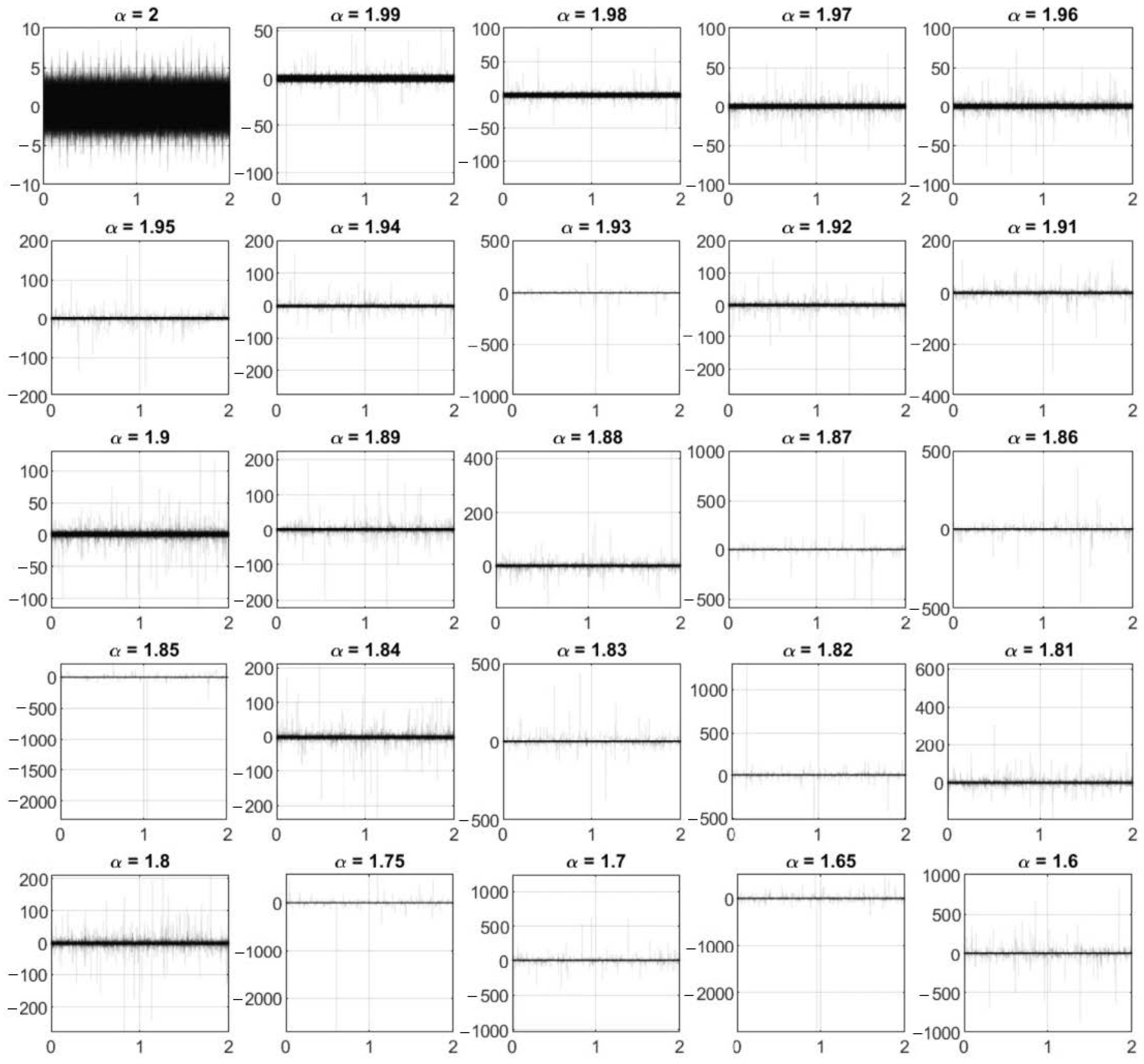
The example of 10 signals (plotted in each 25 figures) prepared for the NMF evaluation for each value of (presented in the titles) and is illustrated in Figure 3.
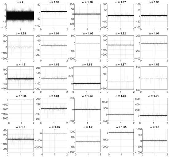
Figure 3.
Exemplary signals prepared for NMF evaluation (note there are 10 signals plotted on each figure), . The vertical axis represents the amplitude, and the horizontal axis refers to the time (in seconds).
The black parts correspond to the overlapping data in contrast to the light gray lines responsible for the random and non-overlapping parts of the signals. The authors decided to select this case because the SOI is hardly visible (but still possible to see) over the noise. This is especially evident when = 2, i.e., when the noise is Gaussian and there are no random impulses present in the signals. While the parameter decreases, it can be observed that both the number and the amplitude of random impulses increase and the visibility of the SOI decreases.
Exemplary spectrograms for and the varying parameter are presented in Figure 4. Note that, for the same pair of and , the spectrograms are different, since we are dealing with a random process. For better visibility, the authors selected 12 values of . The impulses corresponding to the fault are represented by the cyclic vertical lines (they are visible with period T = s and a center frequency of kHz). As one can see, when parameter decreases, the vertical lines are covered by the increasing non-Gaussian noise.
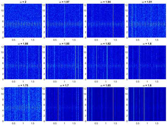
Figure 4.
Exemplary spectrograms for selected values of ; . The vertical axis represents the frequencies (in kHz) and the horizontal axis denotes the time (in seconds). Note, that colour of each pixel on the map is related to the amplitude of given component, more hot colour, higher amplitude.
The base and encoding vectors for both examined NMF methods are illustrated in Figure 5 and Figure 6. The ENVSI measure was used to select the proper class, i.e., corresponding to the SOI. The authors assume that the highest value of this indicator is responsible for the fault. As can be observed, both base and encoding vectors for -HALS NMF present acceptable results for lower values of (in -HALS NMF, the IFB and SOI are visible while in the standard NMF they are not). Moreover, if they point to the proper center frequency in the base vectors and cyclic modulations in the encoding vectors, the vector maps are in most cases less noisy than in the standard NMF (observed visually only). This property is not taken into account when calculating the efficiency of the algorithms, since the main goal was to determine whether the method can detect the damage or not. However, it is also an important aspect.
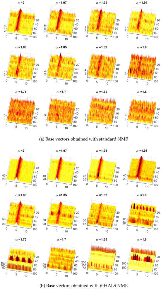
Figure 5.
Base vectors obtained with the standard (top panel) and -HALS NMF (bottom panel) for 100 trials and selected values of . The ENVSI measure was used to select the class corresponding to the fault.
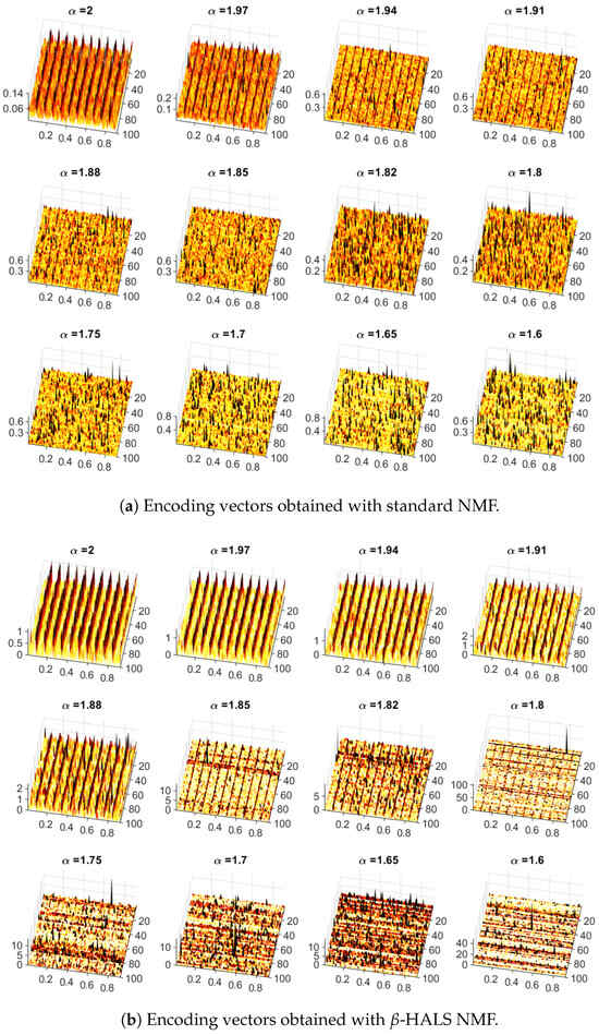
Figure 6.
Encoding vectors obtained with the standard (top panel) and -HALS NMF (bottom panel) for 100 trials and selected values of . The ENVSI measure was used to select the class corresponding to the fault.
3.2. Real Data Analysis
In this section, the authors present the results of two cases corresponding to acoustic and vibration analysis, respectively. In the first case, the acoustic signal was captured from an idler with faulty bearings. The idlers are rotating elements of the conveyor structure that support the belt to transport the material. Each idler is made up of a shaft, two bearings, and a coating. The design of belt conveyors makes the number of idlers massive in practice. This leads to the need for a quick method that would make it possible to diagnose them without disrupting their operation. An automatic, quick, and contactless assessment of their condition would make it possible to schedule replacement so as not to interfere with belt conveyor operations. Until now, the inspection has been performed in a classical way—the evaluation is carried out visually using human senses (sight and hearing) by a maintenance expert.
The measurements were obtained using a typical smartphone. In fact, the video was recorded and the sound extracted from it. The experiment consisted of measuring the sound of 10 s duration for each idler, with the sampling frequency kHz. The real-life belt conveyor is presented in Figure 7 (left). The belt located on it is joined by a metal clip (marked with a red frame). When it passes through the idler, there is interference in the sound signal (as illustrated on the right side).
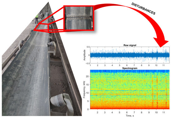
Figure 7.
Real-life belt conveyor (left side) and raw acoustic data with corresponding spectrogram (right side).
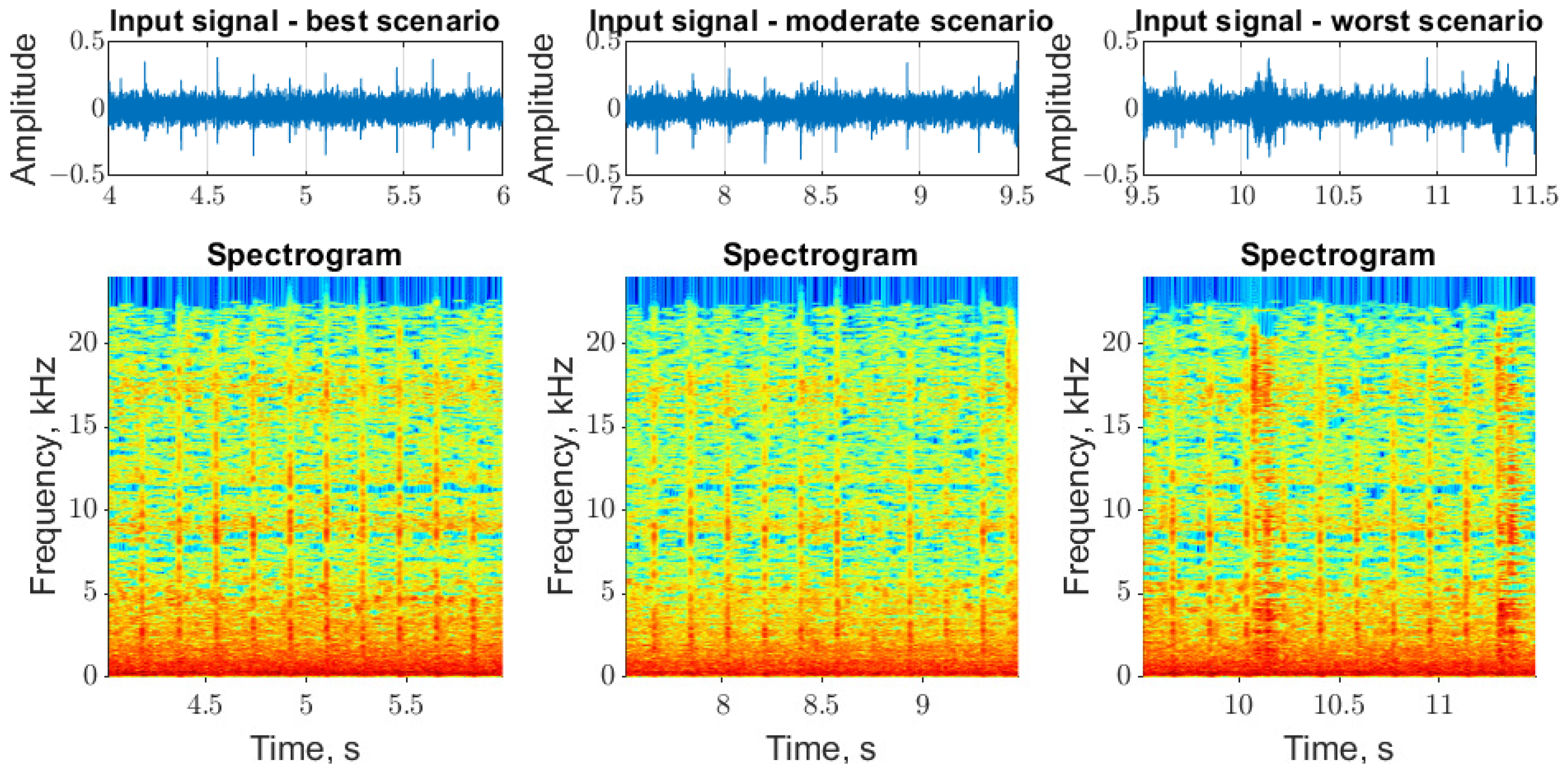
The NMF analysis was performed on the real data acoustic signal divided into three scenarios (see Figure 8). The estimation of parameter in the cases analyzed was carried out using the Koutrouvelis method [54].
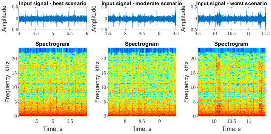
Figure 8.
Selected input signals (top panels) and corresponding spectrograms (bottom panels).
- The first part between 4–6 s is labeled as the best scenario. All the cyclic impulses are clearly visible in the time series and the corresponding spectrogram; thus, high-quality results are expected for both NMF methods. The estimated value of is equal to 1.975.
- The second part between 7.5 and 9.5 s is labeled as the moderate scenario. Most of the cyclic impulses are clearly visible, but two of them are hidden within the noise. At the end of the signal, one of the disturbances corresponding to the metal clip can be observed. The estimated value of is equal to 1.963.
- The third part between 9.5 and 11.5 s is labeled as the worst scenario. As one can observe, two high-energy and non-cyclic impulses are present in this segment. They occur at the same time as the cyclic impulses and cover them up. The estimated value of is equal to 1.916.
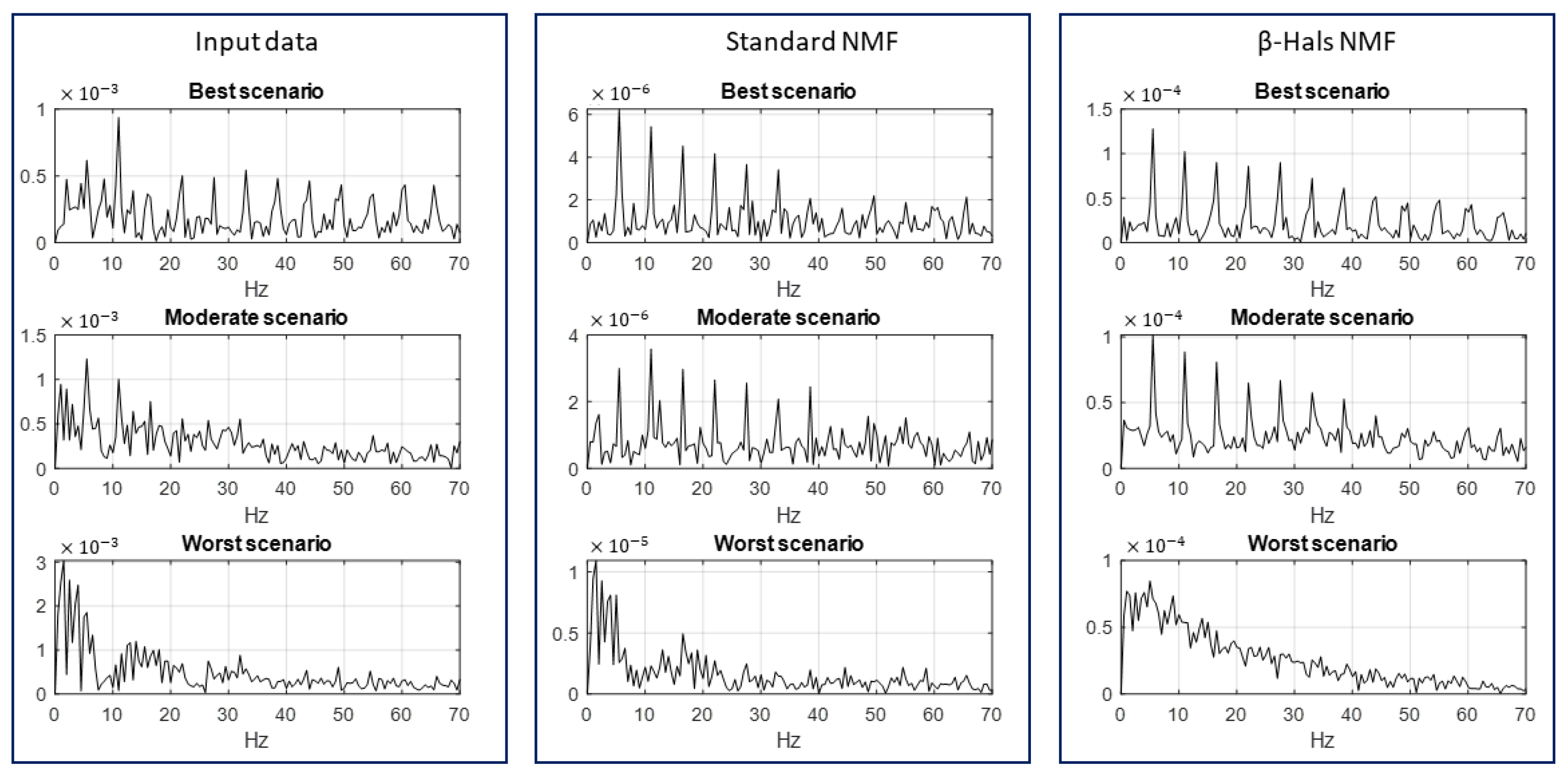
Figure 9 displays the envelope spectra for three scenarios, obtained using the input data and both analyzed NMF algorithms. In the best scenario, when no disturbances are observed in the signal, both models allow us to obtain the correct and clear results; however, -HALS NMF has a lower level of noise—more harmonics can be observed. The moderate scenario is more challenging. Due to the hidden impulses and slight disturbance, the obtained envelope spectra are less clear but still make it possible to detect the fault correctly. In the third selected part, the situation is complicated. The random disturbance that comes from the metal clip efficiently impedes correct detection by using the tested algorithms.
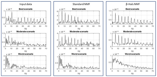
Figure 9.
Envelope spectra obtained by the input data (left panels), standard NMF (middle panels), and -HALS NMF (right panels) for each scenario. The spectra corresponding to the signals in Figure 8.
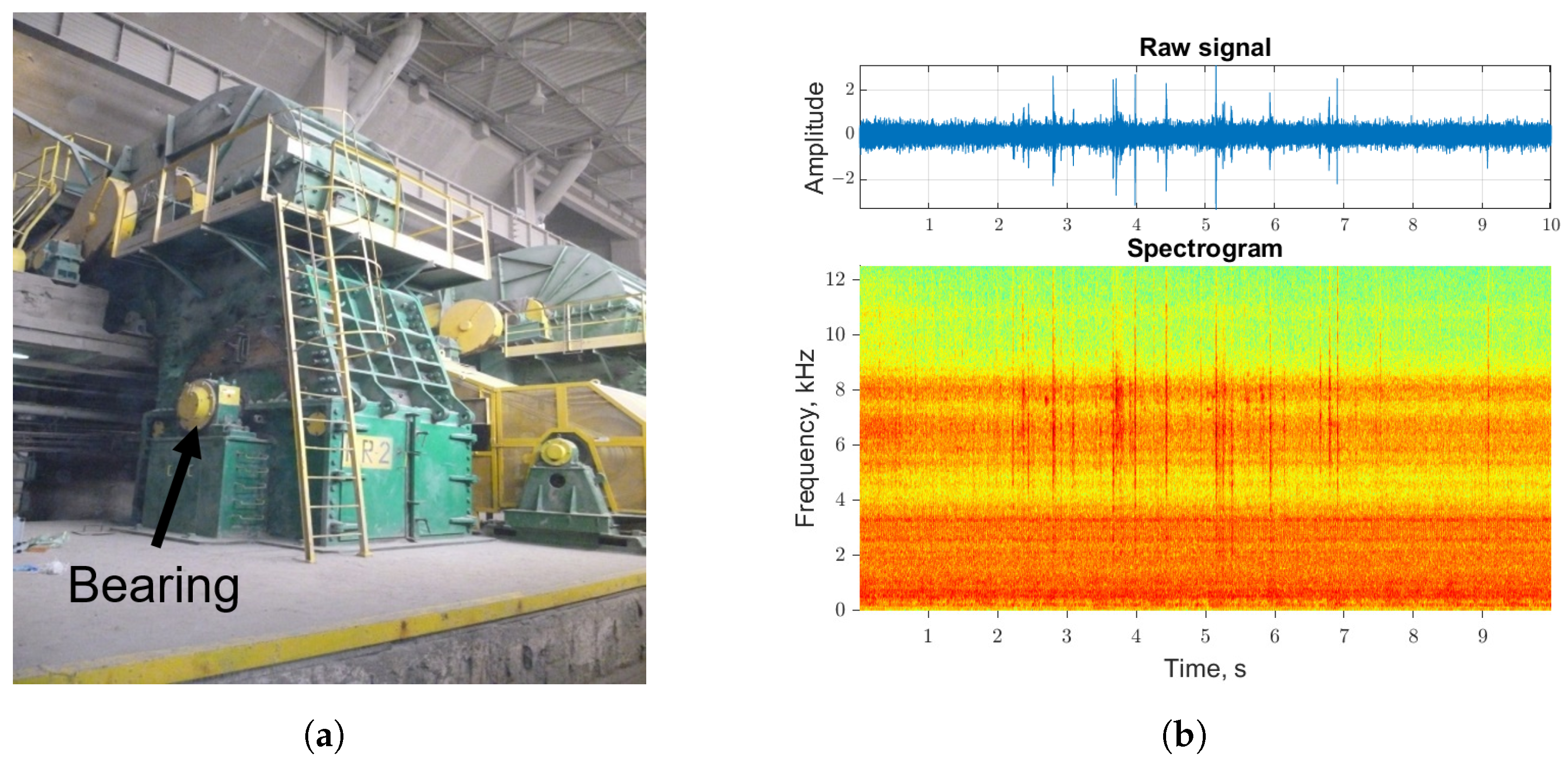
In the second case, the vibration signal was captured from a copper ore crusher (see Figure 10a). Measurements were made using LabView 2015 software and the National Instruments data acquisition module (NiDAQ) with a sampling frequency of kHz. The Endevco accelerometers, which were mounted on magnets, were used to acquire acceleration signals. From all the measurements, the 10 s segment was selected (see Figure 10b).
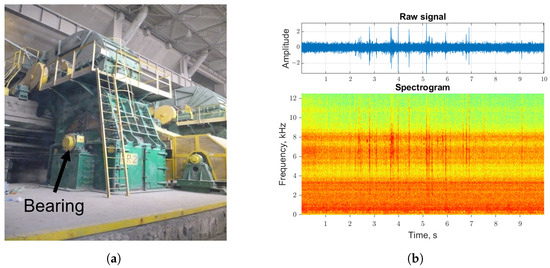
Figure 10.
Real-life copper ore crusher (panel a) and input signal with corresponding spectrogram (panel b).
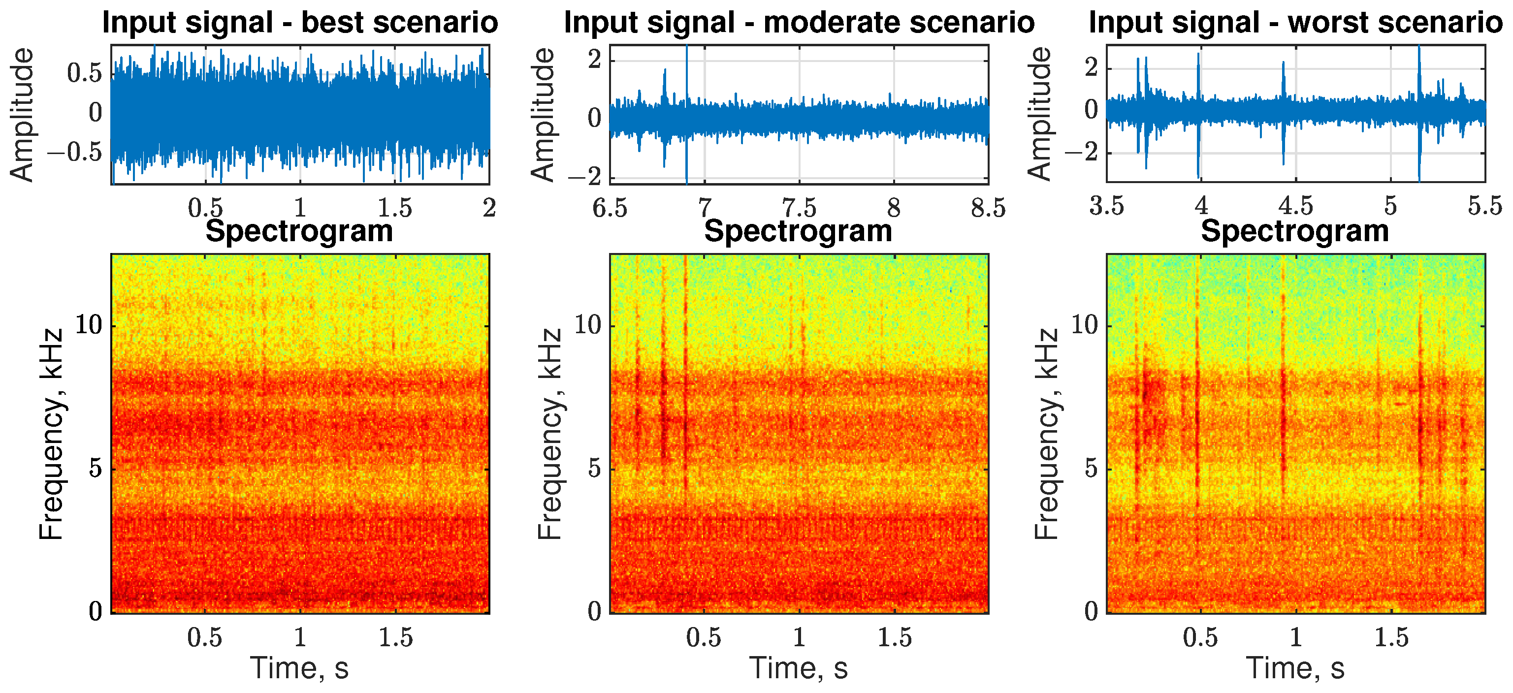
In the vibration data, as in the previous case with the acoustic data, three two-second segments of the signal have been selected, taking into account the amount of non-cyclic disturbances (see Figure 11). They are associated with the normal operation of the machine and are induced by the falling ore—larger pieces cause bigger shocks.
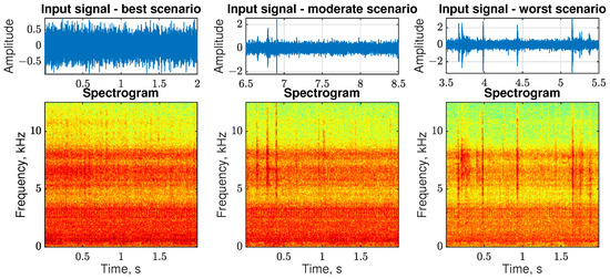
Figure 11.
Selected input signals (top panels) and corresponding spectrograms (bottom panels).
- The best scenario takes place between 0 and 2 s. The impulses corresponding to the random shocks are not visible in this part of the signal. The cyclic impulses corresponding to the damage are not clearly visible. The estimated value of is equal to 1.9823.
- The moderate scenario takes place between 6.5 and 8.5 s. As one can observe in the time series, three visible random impulses are present in the time series. The estimated value of is equal to 1.9418.
- The worst scenario takes place between 3.5 and 5.5 s. This part is strongly contaminated with high-energy impulses. The estimated value of is equal to 1.7630.
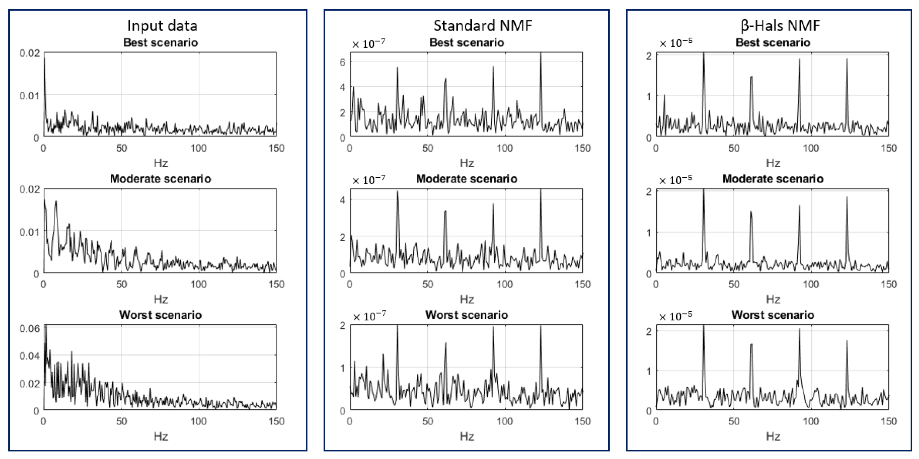
The fault-related component is not easily identifiable without a more in-depth analysis. The envelope spectra of the input data, as shown in the right panels of Figure 12, do not facilitate the detection of damage. In all scenarios, both NMF models allow us to identify the component corresponding to the damage; however, -HALS NMF provides clearer results.
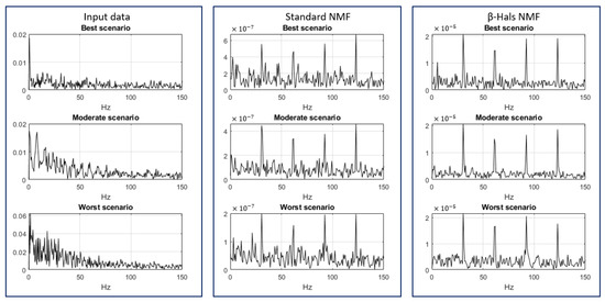
Figure 12.
Envelope spectra obtained by the input data (left panels), standard NMF (middle panels), and -HALS NMF (right panels) for each scenario.
4. Discussion
The visual representation of the results presented in Figure 5 and Figure 6 gives information on the quality of the results. However, to evaluate NMF with respect to the quality of informative signal extraction, an answer to the following questions is needed: which of these algorithms is more efficient under difficult conditions? What level of non-Gaussianity may provide acceptable results?
The authors discuss how both analyzed parameters impact SOI extraction. For this purpose, Monte Carlo (MC) simulations have been carried out with 100 runs for each value of the stability index and the scale parameter and, finally, the efficiency of the methods was determined. The efficiency was calculated on the basis of the ENVSI that was applied for each reconstructed time series. This measure returns higher values when the recovered signal is more informative. Therefore, the indicator value was counted for each of the reconstructed signals (one for each rank) and sorted. The cut-off value that determines whether the indicator corresponds to the signal that allows fault detection has been set manually.
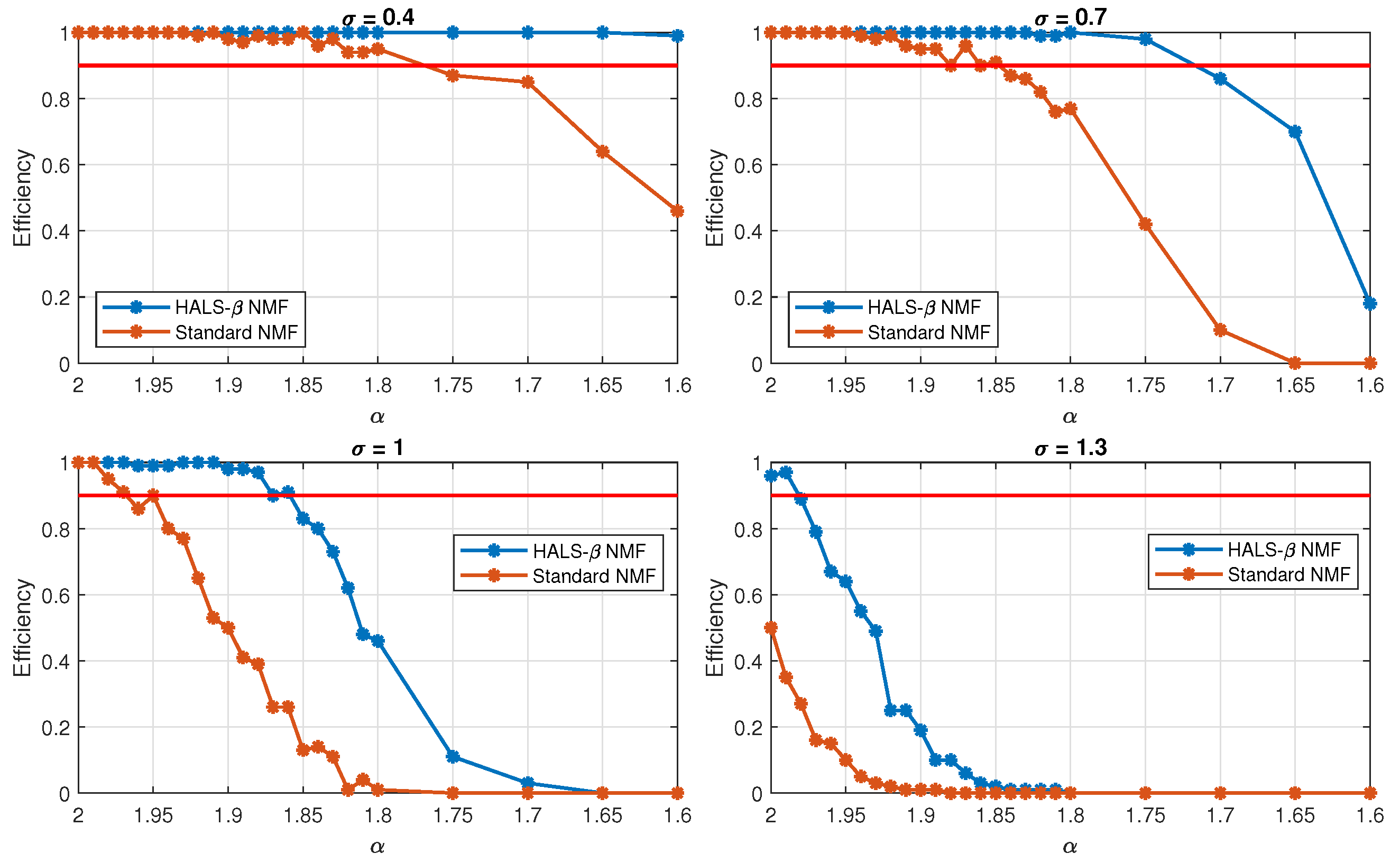
The efficiency of both NMF algorithms analyzed for 25 levels of and 4 levels of is shown in Figure 13. The red horizontal line corresponds to the efficiency of 90%. The interpretation of the obtained results can be divided into 4 groups, depending on the scale parameter.
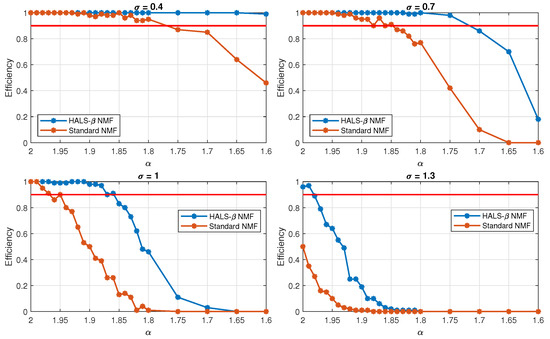
Figure 13.
Efficiency of both tested NMF algorithms (i.e., HALS- NMF and Standard NMF) for 4 levels of and 25 levels of . The efficiency of 90% is represented by the red horizontal line.
- For both NMF methods give high-quality results. The efficiency of -HALS NMF does not decrease, even in the case of a strong non-Gaussian signal (). For the standard NMF, while parameter is lower than , the efficiency decreases. In the worst case analyzed here, the SOI is properly extracted in 46 simulations. In the input time series, the cyclic impulses are clearly visible over the noise level (see the upper left panel of Figure 2).
- For 0.7 and in range , both algorithms show the acceptable results (above 90%). As expected, if the stability index decreases, the effectiveness of both tested NMF methods decreases. Nevertheless, the acceptable result can be observed for -HALS NMF as long as is greater than 1.75.
- For , -HALS NMF yields the acceptable results for . In addition, the fluctuations are slight in a given range. The situation is different in the case of the second tested method—standard NMF. Here, starting from the very beginning, the efficiency decreases, which means that the obtained results quickly cease to be reliable.
- For , when the cyclic impulses are fully hidden in the noise, both NMF methods produce low quality results. For an equal to 1.88, the standard NMF does not show any correct result. The other algorithm, -HALS NMF, achieves better results, but only for the two highest values of has the effectiveness above 90%. However, in the case where the SOI is fully hidden in the strong non-Gaussian noise, both tested algorithms are not suitable for diagnostic purposes (see the bottom right panel in Figure 2).
Analyzing the results, it is important to note that there is a random initialization in NMF algorithms [37] and the NMF optimization problem is intrinsically non-convex, so MC simulations are necessary. In Section 3.2, the analysis performed on real data confirmed the results obtained in the simulations. The more a non-Gaussian signal is observed, the lower the effectiveness of the tested methods. In addition, -HALS NMF is usable for a wider range of values, that is, it is capable of correctly and more clearly detecting damage for the non-Gaussian case. The authors of the previous work proposed the algorithm based on the -HALS NMF dedicated to local damage detection in the presence of heavy-tailed impulsive noise [55]. Before this algorithm was selected, several different NMF models, which are computationally simpler, were investigated. Unfortunately, none of them were able to produce an acceptable level of separability between the vectors. That analysis was performed and tested involving the real data vibration signal coming from the hammer crusher used in the mining industry. In relation to the mentioned article, the results of this paper confirm the assertion that the selected NMF algorithm (-HALS NMF) is suitable for the considered scenarios (SOI in the presence of non-Gaussian noise).
Parameter for the -HALS NMF was set to 1, which corresponds to the Euclidean distance. However, as shown in the literature [56], other metrics might be preferable for non-Gaussian noise. For , the Itakura–Saito distance can be obtained, which is commonly used for the analysis of spectrograms. However, in the case of strongly non-Gaussian (-stable) noise, no performance improvement was observed with the use of this distance. In further studies, the authors plan to test the behavior of NMF algorithms based on the -divergence for other non-Gaussian distributions (e.g., generalized Student’s t-distribution, etc.).
5. Conclusions
In this study, the influence of -stable noise on the effectiveness of NMF is discussed. The authors take this issue under investigation because the non-Gaussian noise effectively complicates the damage detection in machines with rotating elements for many well-known techniques.
The main purpose of this study was to recognize the range of parameters for which the NMF algorithms allow us to correctly separate vectors with the damage signature (i.e., how small parameter can be). Using the simple additive model and MC simulations, the effectiveness of two NMF methods was obtained. Putting together the four scenarios analyzed, the effectiveness of both NMF algorithms depends on both parameters and . Moreover, -HALS NMF returns better results in almost every case analyzed. Only for , , and , are the results of both techniques comparable. The fault detection efficiency is the same (100%), but the standard NMF results are more contaminated with noise.
Furthermore, the authors selected the real acoustic data that come from the belt conveyor. The metal clip on the belt, when it passes an idler, creates the disturbances present in the signal. For the hammer crusher in the vibration data, the disturbances are caused by the ore. Three two-second fragments with different levels of non-Gaussianity were selected from the acoustic and vibration signal to verify the results obtained during the simulation.
It should be emphasized that the tested model is only a simplification: the authors assume that, during the simulation, parameters and do not change. However, the discussed parameters may change over time in real acoustic and vibration signals. Researchers must pay particular attention while selecting the part of the signal for analysis. Finally, it can be concluded that the results obtained during the simulation and the analysis of real data confirm that the efficiency of -HALS NMF algorithm is higher than that of standard NMF.
Author Contributions
Conceptualization, A.M., R.Z. (Rafał Zdunek), R.Z. (Radosław Zimroz) and A.W.; Methodology, A.M. and R.Z. (Radosław Zimroz); Software, A.M., R.Z. (Radosław Zimroz) and A.W.; Validation, A.W.; Formal analysis, R.Z. (Rafał Zdunek) and A.W.; Investigation, A.M.; Resources, A.M. and R.Z. (Radosław Zimroz); Data curation, A.M.; Writing—original draft, A.M., R.Z. (Radosław Zimroz), R.Z. (Rafał Zdunek) and A.W.; Writing—review & editing, A.M., R.Z. (Radosław Zimroz) and R.Z. (Rafał Zdunek); Visualization, A.M.; Supervision, R.Z. (Rafał Zdunek), R.Z. (Radosław Zimroz) and A.W.; Project administration, R.Z. (Radosław Zimroz) and A.W.; Funding acquisition, R.Z. (Radosław Zimroz) and A.W. All authors have read and agreed to the published version of the manuscript.
Funding
This work is supported by the National Center of Science under Sheng2 project No. UMO-2021/40/Q/ST8/00024 “NonGauMech—New methods of processing non-stationary signals (identification, segmentation, extraction, modeling) with non-Gaussian characteristics for the purpose of monitoring complex mechanical structures”.
Data Availability Statement
Data are contained within the article.
Conflicts of Interest
The authors declare no conflicts of interest.
References
- Gundewar, S.K.; Kane, P.V. Bearing fault diagnosis using time segmented Fourier synchrosqueezed transform images and convolution neural network. Measurement 2022, 203, 111855. [Google Scholar] [CrossRef]
- Zheng, J.; Huang, S.; Pan, H.; Tong, J.; Wang, C.; Liu, Q. Adaptive power spectrum Fourier decomposition method with application in fault diagnosis for rolling bearing. Measurement 2021, 183, 109837. [Google Scholar] [CrossRef]
- Randall, R.B.; Antoni, J. Rolling element bearing diagnostics—A tutorial. Mech. Syst. Signal Process. 2011, 25, 485–520. [Google Scholar] [CrossRef]
- Antoni, J. Cyclic spectral analysis of rolling-element bearing signals: Facts and fictions. J. Sound Vib. 2007, 304, 497–529. [Google Scholar] [CrossRef]
- Antoni, J. The spectral kurtosis: A useful tool for characterising non-stationary signals. Mech. Syst. Signal Process. 2006, 20, 282–307. [Google Scholar] [CrossRef]
- Hebda-Sobkowicz, J.; Zimroz, R.; Pitera, M.; Wylomanska, A. Informative frequency band selection in the presence of non-Gaussian noise—A novel approach based on the conditional variance statistic with application to bearing fault diagnosis. Mech. Syst. Signal Process. 2020, 145, 106971. [Google Scholar] [CrossRef]
- Obuchowski, J.; Wyłomańska, A.; Zimroz, R. Selection of informative frequency band in local damage detection in rotating machinery. Mech. Syst. Signal Process. 2014, 48, 138–152. [Google Scholar] [CrossRef]
- Antoni, J. Fast computation of the kurtogram for the detection of transient faults. Mech. Syst. Signal Process. 2007, 21, 108–124. [Google Scholar] [CrossRef]
- Antoni, J. The infogram: Entropic evidence of the signature of repetitive transients. Mech. Syst. Signal Process. 2016, 74, 73–94. [Google Scholar] [CrossRef]
- Zhao, M.; Lin, J.; Miao, Y.; Xu, X. Detection and recovery of fault impulses via improved harmonic product spectrum and its application in defect size estimation of train bearings. Measurement 2016, 91, 421–439. [Google Scholar] [CrossRef]
- Miao, Y.; Zhao, M.; Lin, J. Improvement of kurtosis-guided-grams via Gini index for bearing fault feature identification. Meas. Sci. Technol. 2017, 28, 125001. [Google Scholar] [CrossRef]
- Bozchalooi, I.S.; Liang, M. A smoothness index-guided approach to wavelet parameter selection in signal de-noising and fault detection. J. Sound Vib. 2007, 308, 246–267. [Google Scholar] [CrossRef]
- Moshrefzadeh, A.; Fasana, A. The Autogram: An effective approach for selecting the optimal demodulation band in rolling element bearings diagnosis. Mech. Syst. Signal Process. 2018, 105, 294–318. [Google Scholar] [CrossRef]
- Wang, X.; Zheng, J.; Ni, Q.; Pan, H.; Zhang, J. Traversal index enhanced-gram (TIEgram): A novel optimal demodulation frequency band selection method for rolling bearing fault diagnosis under non-stationary operating conditions. Mech. Syst. Signal Process. 2022, 172, 109017. [Google Scholar] [CrossRef]
- Liu, W.; Yang, S.; Liu, Y.; Gu, X. DTMSgram: A novel optimal demodulation frequency band selection method for wheelset bearings fault diagnosis under wheel-rail excitation. Meas. Sci. Technol. 2024, 35, 045105. [Google Scholar] [CrossRef]
- Cui, L.; Zhao, X.; Liu, D.; Wang, H. A spectral coherence cyclic periodic index optimization-gram for bearing fault diagnosis. Measurement 2024, 224, 113898. [Google Scholar] [CrossRef]
- Yu, G.; Li, C.; Zhang, J. A new statistical modeling and detection method for rolling element bearing faults based on alpha–stable distribution. Mech. Syst. Signal Process. 2013, 41, 155–175. [Google Scholar] [CrossRef]
- Schmidt, S.; Mauricio, A.; Heyns, P.S.; Gryllias, K.C. A methodology for identifying information rich frequency bands for diagnostics of mechanical components-of-interest under time-varying operating conditions. Mech. Syst. Signal Process. 2020, 142, 106739. [Google Scholar] [CrossRef]
- Schmidt, S.; Heyns, P.S.; Gryllias, K.C. An informative frequency band identification framework for gearbox fault diagnosis under time-varying operating conditions. Mech. Syst. Signal Process. 2021, 158, 107771. [Google Scholar] [CrossRef]
- Mauricio, A.; Smith, W.A.; Randall, R.B.; Antoni, J.; Gryllias, K. Improved Envelope Spectrum via Feature Optimisation-gram (IESFOgram): A novel tool for rolling element bearing diagnostics under non-stationary operating conditions. Mech. Syst. Signal Process. 2020, 144, 106891. [Google Scholar] [CrossRef]
- Michalak, A.; Wodecki, J.; Drozda, M.; Wyłomańska, A.; Zimroz, R. Model of the vibration signal of the vibrating sieving screen suspension for condition monitoring purposes. Sensors 2020, 21, 213. [Google Scholar] [CrossRef]
- Antoni, J. Cyclic spectral analysis in practice. Mech. Syst. Signal Process. 2007, 21, 597–630. [Google Scholar] [CrossRef]
- Abboud, D.; Antoni, J.; Eltabach, M.; Sieg-Zieba, S. Angle/time cyclostationarity for the analysis of rolling element bearing vibrations. Measurement 2015, 75, 29–39. [Google Scholar] [CrossRef]
- Kruczek, P.; Zimroz, R.; Antoni, J.; Wyłomańska, A. Generalized spectral coherence for cyclostationary signals with α-stable distribution. Mech. Syst. Signal Process. 2021, 159, 107737. [Google Scholar] [CrossRef]
- Liu, T.H.; Mendel, J.M. A subspace-based direction finding algorithm using fractional lower order statistics. IEEE Trans. Signal Process. 2001, 49, 1605–1613. [Google Scholar]
- Chen, Z.; Geng, X.; Yin, F. A Harmonic Suppression Method Based on Fractional Lower Order Statistics for Power System. IEEE Trans. Ind. Electron. 2016, 63, 3745–3755. [Google Scholar] [CrossRef]
- Aalo, V.A.; Ackie, A.B.E.; Mukasa, C. Performance analysis of spectrum sensing schemes based on fractional lower order moments for cognitive radios in symmetric α-stable noise environments. Signal Process. 2019, 154, 363–374. [Google Scholar] [CrossRef]
- Das, S.; Pan, I. Fractional Order Signal Processing: Introductory Concepts and Applications; Chapter Fractional Order Statistical Signal Processing; Springer: Berlin/Heidelberg, Germany, 2012; pp. 83–96. [Google Scholar]
- Ma, X.; Nikias, C.L. Joint estimation of time delay and frequency delay in impulsive noise using fractional lower order statistics. IEEE Trans. Signal Process. 1996, 44, 2669–2687. [Google Scholar]
- Luan, S.; Qiu, T.; Zhu, Y.; Yu, L. Cyclic correntropy and its spectrum in frequency estimation in the presence of impulsive noise. Signal Process. 2016, 120, 503–508. [Google Scholar] [CrossRef]
- Liu, T.; Qiu, T.; Luan, S. Cyclic Correntropy: Foundations and Theories. IEEE Access 2018, 6, 34659–34669. [Google Scholar] [CrossRef]
- Fontes, A.I.; Rego, J.B.; de M. Martins, A.; Silveira, L.F.; Principe, J. Cyclostationary correntropy: Definition and applications. Expert Syst. Appl. 2017, 69, 110–117. [Google Scholar] [CrossRef]
- Mehmood, A.; Damarla, T. Kernel non-negative matrix factorization for seismic signature separation. J. Pattern Recognit. Res. 2013, 8, 13–25. [Google Scholar] [CrossRef] [PubMed]
- Liang, L.; Shan, L.; Liu, F.; Niu, B.; Xu, G. Sparse envelope spectra for feature extraction of bearing faults based on nmf. Appl. Sci. 2019, 9, 755. [Google Scholar] [CrossRef]
- Liang, L.; Shan, L.; Liu, F.; Li, M.; Niu, B.; Xu, G. Impulse Feature Extraction of Bearing Faults Based on Convolutive Nonnegative Matrix Factorization. IEEE Access 2020, 8, 88617–88632. [Google Scholar] [CrossRef]
- Gu, X.; Yang, S.; Liu, Y.; Hao, R.; Liu, Z. Multi-objective Informative Frequency Band Selection Based on Negentropy-induced Grey Wolf Optimizer for Fault Diagnosis of Rolling Element Bearings. Sensors 2020, 20, 1845. [Google Scholar] [CrossRef]
- Wodecki, J.; Michalak, A.; Zimroz, R.; Barszcz, T.; Wyłomańska, A. Impulsive source separation using combination of Nonnegative Matrix Factorization of bi-frequency map, spatial denoising and Monte Carlo simulation. Mech. Syst. Signal Process. 2019, 127, 89–101. [Google Scholar] [CrossRef]
- Wang, X.; Cai, Y.; Li, A.; Zhang, W.; Yue, Y.; Ming, A. Intelligent fault diagnosis of diesel engine via adaptive VMD-Rihaczek distribution and graph regularized bi-directional NMF. Measurement 2021, 172, 108823. [Google Scholar] [CrossRef]
- Li, B.; Zhang, P.l.; Liu, D.s.; Mi, S.s.; Ren, G.q.; Tian, H. Feature extraction for rolling element bearing fault diagnosis utilizing generalized S transform and two-dimensional non-negative matrix factorization. J. Sound Vib. 2011, 330, 2388–2399. [Google Scholar] [CrossRef]
- Wei, Y.; Xu, Y.; Hou, Y.; Li, L. Improved Adaptive Multipoint Optimal Minimum Entropy Deconvolution and Application on Bearing Fault Detection in Random Impulsive Noise Environments. Entropy 2023, 25, 1171. [Google Scholar] [CrossRef]
- Zhao, X.; Qin, Y.; He, C.; Jia, L.; Kou, L. Rolling element bearing fault diagnosis under impulsive noise environment based on cyclic correntropy spectrum. Entropy 2019, 21, 50. [Google Scholar] [CrossRef]
- Cichocki, A.; Zdunek, R.; Phan, A.H.; Amari, S.I. Nonnegative Matrix and Tensor Factorizations: Applications to Exploratory Multi-Way Data Analysis and Blind Source Separation; John Wiley & Sons: Hoboken, NJ, USA, 2009. [Google Scholar]
- Cichocki, A.; Phan, A.H.; Caiafa, C. Flexible HALS algorithms for sparse non-negative matrix/tensor factorization. In Proceedings of the 2008 IEEE Workshop on Machine Learning for Signal Processing, Cancun, Mexico, 16–19 October 2008; pp. 73–78. [Google Scholar]
- Cichocki, A.; Phan, A.H. Fast local algorithms for large scale nonnegative matrix and tensor factorizations. IEICE Trans. Fundam. Electron. Commun. Comput. Sci. 2009, 92, 708–721. [Google Scholar] [CrossRef]
- Samorodnitsky, G.; Taqqu, M.S. Stable Non-Gaussian Random Processes: Stochastic Models with Infinite Variance; Chapman & Hall: New York, NY, USA, 1994. [Google Scholar]
- Weron, A. Stable processes and measures; A survey. In Proceedings of the Probability Theory on Vector Spaces III, Lublin, Poland, 24–31 August 1983; Szynal, D., Weron, A., Eds.; Springer: Berlin/Heidelberg, Germany, 1984; pp. 306–364. [Google Scholar]
- Zolotarev, V.M. One-Dimensional Stable Distributions; Translations of Mathematical Monographs; American Mathematical Society: Providence, RI, USA, 1986. [Google Scholar]
- Weron, A.; Weron, R. Computer simulation of Lévy α-stable variables and processes. In Chaos—The Interplay between Stochastic and Deterministic Behaviour: Proceedings of the XXXIst Winter School of Theoretical Physics Held in Karpacz, Poland, 13–24 February 1995; Springer: Berlin/Heidelberg, Germany, 2005; pp. 379–392. [Google Scholar]
- Allen, J. Short term spectral analysis, synthesis, and modification by discrete Fourier transform. IEEE Trans. Acoust. Speech Signal Process. 1977, 25, 235–238. [Google Scholar] [CrossRef]
- Lee, D.; Seung, S. Algorithms for non-negative matrix factorization. In Advances in Neural Information Processing Systems; The MIT Press: Cambridge, MA, USA, 2001; pp. 556–562. [Google Scholar]
- Griffin, D.; Lim, J. Signal estimation from modified short-time Fourier transform. IEEE Trans. Acoust. Speech Signal Process. 1984, 32, 236–243. [Google Scholar] [CrossRef]
- Crochiere, R. A weighted overlap-add method of short-time Fourier analysis/synthesis. IEEE Trans. Acoust. Speech Signal Process. 1980, 28, 99–102. [Google Scholar] [CrossRef]
- Marple, L. Computing the discrete-time “analytic” signal via FFT. IEEE Trans. Signal Process. 1999, 47, 2600–2603. [Google Scholar] [CrossRef]
- Koutrouvelis, I.A. Regression-type estimation of the parameters of stable laws. J. Am. Stat. Assoc. 1980, 75, 918–928. [Google Scholar] [CrossRef]
- Wodecki, J.; Michalak, A.; Zimroz, R. Local damage detection based on vibration data analysis in the presence of Gaussian and heavy-tailed impulsive noise. Measurement 2021, 169, 108400. [Google Scholar] [CrossRef]
- Févotte, C.; Bertin, N.; Durrieu, J.L. Nonnegative matrix factorization with the Itakura-Saito divergence: With application to music analysis. Neural Comput. 2009, 21, 793–830. [Google Scholar] [CrossRef]


Disclaimer/Publisher’s Note: The statements, opinions and data contained in all publications are solely those of the individual author(s) and contributor(s) and not of MDPI and/or the editor(s). MDPI and/or the editor(s) disclaim responsibility for any injury to people or property resulting from any ideas, methods, instructions or products referred to in the content. |
© 2024 by the authors. Licensee MDPI, Basel, Switzerland. This article is an open access article distributed under the terms and conditions of the Creative Commons Attribution (CC BY) license (https://creativecommons.org/licenses/by/4.0/).