Dynamic Voltage and Frequency Scaling as a Method for Reducing Energy Consumption in Ultra-Low-Power Embedded Systems

Abstract

Dynamic voltage and frequency scaling (DVFS) is a technique used to optimize energy consumption in ultra-low-power embedded systems. To ensure sufficient computational capacity, the system must scale up its performance settings. The objective is to conserve energy in times of reduced computational demand and/or when battery power is used. Fast Fourier Transform (FFT), Cyclic Redundancy Check 32 (CRC32), Secure Hash Algorithm 256 (SHA256), and Message-Digest Algorithm 5 (MD5) are focused functions that demand computational power to achieve energy-efficient performance. Selected operations are analyzed from the energy consumption perspective. In this manner, the energy required to perform a specific function is observed, thereby mitigating the influence of the instruction set or system architecture. For stable operating voltage scaling, an exponential model for voltage calculation is presented. Statistical significance tests are conducted to validate and support the findings. Results show that the proposed optimization technique reduces energy consumption for ultra-low-power applications from 27.74% to up to 47.74%.

1. Introduction

Ultra-low-power systems represent a class of computing and electronic systems engineered to operate on minimal energy consumption, often pushing the boundaries of power efficiency. The development of ultra-low-power systems represents a continuous effort to balance the growing demand for advanced functionalities with the need for sustainable and efficient power consumption. These devices advance the capabilities of modern electronics in various fields, from consumer electronics to industrial applications [1]. DVFS involves dynamical adjustment of the operating frequency and voltage of a processor based on the workload demands. By reducing the frequency and voltage when the processing load is low, and increasing them when the workload demands more performance, the system can achieve a balance between energy efficiency and computational power. This method allows the system to conserve energy during periods of lower activity, extending battery life and minimizing heat generation [2].

DVFS is particularly valuable in applications where energy efficiency improvements are present on a larger scale. Maximizing longevity on limited energy resources is also one of the advantages of DVFS, for example, in Internet of Things (IoT) devices [3,4], wireless sensor nodes [5,6], in mobile devices [7], On-Chip temperature sensors in [8], wearables in [9]. Wearable technologies such as smartwatches, fitness trackers, and medical monitoring devices also rely on ultra-low-power properties and DVFS. In this case, minimal energy consumption and a long battery life are essential. Wireless sensors used in smart homes [10], multicore systems [11], and agriculture [12] are often powered by batteries and need to be energy-efficient to last for years. Medical devices such as pacemakers and blood glucose monitoring implants need to operate continuously, reliably, and with minimal power consumption. In applications such as medical implants or remote sensors, where battery replacement can be impractical or impossible, ultra-low-power design is a determining factor for the longevity of the devices. IoT devices such as smart locks, security systems, thermostats, and lighting systems, also require battery and energy efficient operation. Mobile devices such as smartphones, tablets, and e-readers benefit significantly from extended battery life, which directly improves the user experience. Additionally, the examples mentioned are the motivation for the research and development of this paper.

This paper proposes the use of DFS and/or DVFS for reduction in energy consumption and achieving ultra-low-power properties. The technique is based on the type of load and computational requirements at a given moment. The execution of selected operations is analyzed from the energy consumption perspective. Statistical significance tests are conducted to validate and support the findings. Furthermore, the energy aware embedded system design approach discusses hardware and software aspects of DVFS implementation.

The rest of this paper is structured as follows. A review of the relevant literature on the paper topic and contributions are provided in Section 2. The setup, experimental results, and the discussion are given in Section 3. Finally, Section 4 concludes the paper by stating the reached conclusions and offers suggestions for future work.

2. Related Work

In recent years, there have been several attempts to implement DVFS in microcontrollers, driven by the growing demand for energy-efficient computing in various applications. This trend reflects an increasing focus on reducing power consumption and enhancing battery life, especially in portable and embedded devices, where efficient energy usage is crucial. DVFS has emerged as a viable solution to dynamically adjust the power and performance characteristics of microcontrollers in response to real-time computational demands.

A comparison of hash algorithms using a PIC32 microcontroller, with the prospect of developing a CAN bus authentication technique is presented in [13]. The comparison is mainly focused on cycles per byte and memory space, and tests are carried out on a PIC32-based application. The article can serve as a reference for the selection of an appropriate hash algorithm for various communication and transmission systems. Authors in [6] presented an article on energy management techniques for wireless sensor networks (WSNs) in IoT applications with limited resources. Specifically, the paper experimentally implements a hybrid energy management solution using DVFS and Duty-Cycling techniques to optimize operating conditions during data processing and reduce energy consumption of the transceiver. Selecting a higher operating frequency can lead to more efficient power consumption due to its impact on the duty cycle. With a higher operating frequency, the duty cycle is higher, resulting in less power dissipation during idle phases, despite higher average power consumption. In [14] the dynamic frequency control (DFC) approach in embedded application development is presented. It can yield significant benefits when implemented thoughtfully, and can lead to faster processing times and potential savings in metrics like average current draw, power consumption, and overall energy consumption, depending on the application. In the tested application scenarios, dynamic frequency control reduced execution time by up to 33% and overall energy consumption by up to 49% compared to the default static approach. The authors in [15] used different approach. This article proposes a circuit that provides a digital delay regulation of a digital delay line (DDL) matched with the ring oscillator (RO) that clocks the digital subsystem. In order to ensure that the propagation delay through the DDL matches a time reference, the converter controls the supply voltage of the digital subsystem. This circuit’s objective is to guarantee the CPU’s processing speed for real-time applications while limiting supply voltage. The results of the proposed circuit show that the implementation enables power-conversion efficiencies above 50% at 2.5 $\mathsf{\mu }$W of output power. The use of DVFS to improve the energy-efficiency of hardware accelerators in neural networks, particularly for reducing both static and dynamic power in irregular neural networks is discussed in [16]. Various levels of granularity for DVFS implementation are explored, and a machine learning-driven predictive algorithm is presented as a means to enhance precision. The simulation results indicate that substantial energy savings and power reduction were achieved across AlexNet, VGG16, and ResNet50 models. Specifically, an average dynamic energy savings of 59–66% and an average static power reduction of 69–80% were observed, in comparison to the baseline. A technique called D2VFS which aims to regulate supply voltage and clock frequency of intermittently-computing devices is discussed in [17]. D2VFS dynamically modulates voltage levels based on varying workload and program power demands and concurrently adjusting the switching frequency as needed. D2VFS provides up to 300% shorter completion times for a given workload, up to a two-fold improvement in the number of required checkpoints, and up to a one-sixth smaller energy buffer to complete the same workload, and up to 9% increase in clock cycles per active epoch.

Authors in [18] discussed DVFS techniques, which help in quantifying the consumed energy efficiently and accurately. The paper introduces normalized power to accurately and efficiently calculate the energy saving of the implemented DVFS. The proposed DVFS policy is implemented using an ultra-low-power microcontroller MSP430L5529, and highlights the energy-saving measures based on Panstamp. A higher voltage/frequency can result in a notable 57% increase in normalized power, the power consumption increased by 37% with the increase of frequency. A benchmarking-based investigation of various microcontrollers using a periodic duty cycle model, followed by a deep characterization approach using a four-wire measurement is presented in [19]. The resulting characterization data includes active power consumption, sleep power, data logging power, and peripherals power. Normalized values facilitate the comparison of various microcontroller architectures by showing the energy expenditure for each operation or instruction, regardless of the time taken. Authors in [20] propose the usage of a clock-frequency switching technique that can reduce the energy consumption of microcontroller-based sensor nodes. The concept of reducing energy consumption is based on switching the operating clock between low and high frequencies, depending on the application codes of the microcontroller unit (MCU). The technique showed a reduction of up to 66.9% in MCU energy consumption. High frequency for the data processing of image sensor nodes is beneficial for lowering overall energy consumption. Authors in [21] state that the power savings achieved with DVFS can be quantified. DVFS yields quadratic energy savings and, the system using DVFS finishes the task at the same deadline but does so at a lower energy consumption. The energy savings achieved by DVFS can go as high as 59.02% for active components, such as the VCO (voltage-controlled oscillator) and CPU, which shows that the DVFS scheme works adequately for applications that require data processing. Authors in [22] discuss DVFS as a popular technique for managing power consumption in integrated circuits (ICs). The paper proposes an analytic model to find energy efficient points by taking into account the power overheads induced by the extra circuit costs, consisting of two parameters: frequency scaling factor and operational duty cycle. Additional circuit costs in multi-mode designs result from varying circuit delays at different supply voltages and may lead to additional power consumption.

Usage of DVFS for energy minimization problems for mixed-criticality systems is proposed in [23]. The results suggest that under high system utilization and extra workload, exploring time slack to stretch task executions may be less effective for achieving energy savings. Proposed algorithm finds the optimal processor frequency and the corresponding voltage to minimize the expected energy consumption while maintaining the required task deadlines. The input of the algorithm includes the task model parameters, such as the execution time, and the maximum and minimum frequencies. The output of the algorithm includes the optimal processor frequency and voltage, and the corresponding energy consumption. A DFS method to reduce energy consumption in an Atmel ATmega 16 microcontroller is presented in [24]. This technique can help increase battery life and improve system usefulness. They concluded that energy consumption is reduced with the lowest frequency of 1 MHz, but some of the tasks were not performed according to schedule. Hence, DVFS method is proposed, to ensure real-time constraints were met for executing a robotic application based on ATmega 16.

Authors in [25] presented a management system that can be added on to existing microcontrollers that have no built-in power management support and focus on maintaining the throughput of a microcontroller by adjusting the chip frequency. Authors have tested the 32 instructions of PIC microcontroller independently, it was concluded that each instruction consumed different amounts of energy. The goal of power estimating software is to enable a developer to calculate power consumption at various frequency speeds, with the option to set the maximum frequency to assess power usage at peak levels. The use of on-chip voltage regulators for DVFS in chip multiprocessors (CMP) is presented in [26]. The authors show that on-chip regulators can provide better energy savings compared to traditional off-chip regulators, but there are challenges to their implementation, such as efficiency and output voltage transient characteristics. The paper describes and models these costs and performs a comprehensive analysis of a CMP system with integrated on-chip regulators. A more advanced approach includes an on-chip DC–DC converter which enables DVS [27]. The suggested 3-level converter is a combination of a buck and switched-capacitor converter that allows smaller inductors (1 nH) than a buck while generating a larger range of output voltages compared to a half-mode switched-capacitor converter. Measurements were made for a range of static load current conditions (0.3 to 0.8 A), duty cycles (40 to 65%), switching frequencies (50 to 160 MHz) and number of phases (1 to 4). Resulting efficiency peaks at 77% for low load current conditions at 50% duty cycle.

The authors in [28] introduced a technique that dynamically adjusts CPU voltage and frequency based on runtime memory access statistics, achieving substantial energy savings, especially in memory-bound programs. The exploration and implementation of DVFS in the CloudSim simulator is presented in [29]. This work emphasized the need for energy-aware tools in simulating large and distributed systems, demonstrating the close relationship between DVFS efficiency and hardware architecture. The research on fine-grained DVFS using on-chip regulators [30] reconciled conflicting conclusions about the effectiveness of DVFS at different timescales and scaling speeds. It proposed a fine-grained, microarchitecture-driven DVFS mechanism that adjusts voltage and frequency for individual off-chip memory accesses, showing significant energy savings with minimal performance degradation for memory-intensive workloads. A study focusing on modeling power consumption for DVFS policies [31] presented a mathematical model to estimate power consumption under different DVFS policies. This model aimed to assist users in finding optimal configurations for their applications and energy reduction goals, showing high accuracy compared to real-time measurements. In the context of mobile edge computing, research [32] proposed an optimization framework for offloading tasks from a mobile device to multiple edge devices. It focused on minimizing execution latency and energy consumption by optimizing task allocation and CPU frequency, demonstrating performance improvements in terms of energy consumption and execution latency. A predictive temperature-aware DVFS approach [33] used performance counters in commercial microprocessors to predict localized temperature and adjust voltage/frequency efficiently. This approach provided a software solution for thermal issues detected after layout or fabrication, showing comparable performance to DVFS using thermal sensors. The development of an energy-efficient task scheduling algorithm in DVFS-enabled cloud environments is presented in [34]. This research is focused on creating algorithms that enhance energy efficiency in cloud computing settings, particularly in the context of task scheduling. Lastly, a comprehensive survey of energy-aware scheduling algorithms for real-time systems [35] provided a taxonomy to classify existing approaches and discussed challenges related to the evolution towards multicore architectures. This survey covered developments from the mid-1990s to the present, highlighting the evolution of solutions in response to changing platform features and needs.

Contributions of this paper includes energy analysis in scope of computing loads such as FFT128, FFT32, CRC32, MD5 and SHA256. Furthermore, when it comes to dynamic voltage scaling, a exponential model for voltage calculation is presented. To achieve ultra-low-power properties of embedded system, a method for dynamic voltage and frequency scaling based on load requirements has been developed. Load execution is energy governed, and performance level is adjusted to minimize energy usage for each specific load. Described approach can be applicable to other types of embedded systems. Additionally, we give performance per watt (PPW) analysis, with the objective of determining the ideal balance between the energy used and the performance achieved.

3. Experimental Analysis and Discussion

This chapter describes the used experimental setup and the approach applied in the analysis. Examples of real-world operations are used as a basis for energy measurements. With the achieving ultra-low-power properties as the main focus, energy measurements and energy savings for the application of DFS and DVFS are presented in this chapter. PPW analysis for newly developed embedded systems is one of the key elements that can be used to reduce energy consumption at certain loads.

In this study comparison to related work isn’t present, as source code of related articles is often not available or accessible, and there are also differences in hardware platform being used, so the direct comparison wouldn’t result in relevant conclusion.

3.1. Setup

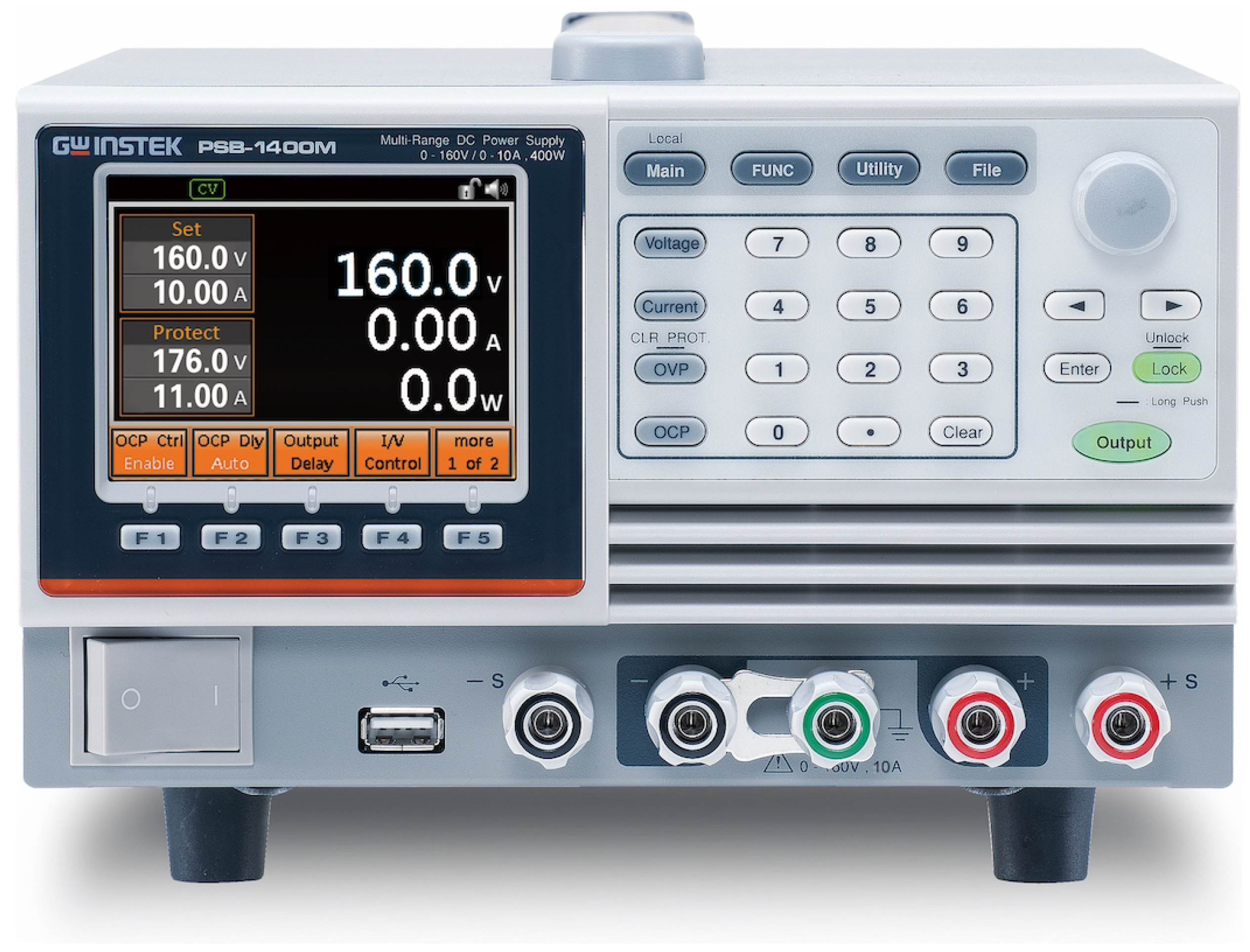
For measurement purposes, Keysight 34465A multimeter is used which can be seen in Figure 1. It features 6 ½ digits of resolution with a maximum read speed of 50,000 readings/s. When it comes to accuracy, datasheet states basic DCV accuracy of 30 parts per million (ppm) [36]. For precise DC supply, programmable multi-range GW INSTEK PSB-1400L DC power supply is used, which can be seen in Figure 2. It features output voltage from 0 to 40 V, and output current from 0 to 40 A, with total power of 400 W. 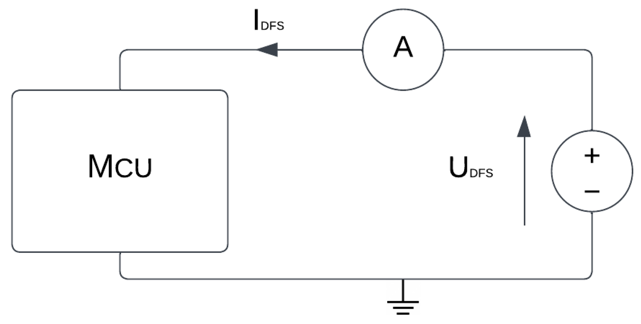It also features voltage measurement accuracy of 0.1% and current measurement accuracy 0.1%, which is relevant when it comes to performing measurements and ensuring repeatable results [37]. Furthermore, connections made for measurements are shown in Figure 3. Ampermeter symbol represents Keysight multimeter, while DC voltage source symbol represents GW Instek programmable DC power supply.

Figure 1. Keysight 34465A desktop multimeter.

Figure 2. GW INSTEK PSB-1400L power supply.

Figure 3. Measurement setup diagram.

The selected MCU is ARM Cortex-M0+ ultra-low-power STM32L0 [38]. The used development environment is STM32CubeIDE, which enables dynamical code generation based on defined Pinout and Configuration. This feature enabled the use of different clock configurations for DFS. The IDE includes advanced debugging capabilities with breakpoints, watchpoints, real-time variable monitoring, and system analysis tools used for the implementation of selected operations, and execution time measurements.

3.2. Dynamic Frequency Scaling

Dynamic frequency scaling (DFS) is adaptive method that offers several advantages, including energy efficiency, reduced thermal load, improved performance in dynamic environments, and decreased noise levels. In our case it is used to improve energy efficiency, which is achievable without any additional hardware changes. Measuring values which are in the focus are operational frequencies, measured current, fixed operating voltage of 3.3 V and execution times for operations FFT128, FFT32, CRC32, MD5 and SHA256.

FFT [39] is represented with pseudocode in Algorithm 1, where FFT128 and FFT32 refer to a sample size of 128 and 32, respectively. CRC32 [40] that generates 32-bit hash value is represented with pseudocode in Algorithm 2. Produced 32-bit hash is often used as a checksum to verify the integrity of data. MD5 [41], a widely-used cryptographic hash function that produces a 128-bit (16-byte) hash value is represented in Algorithm 3. SHA-256 [42], a cryptographic hash function that generates a 256-bit (32-byte) hash value is represented in Algorithm 4. This algorithm takes input data of any length and produces a unique, fixed-length 256-bit hash. Input data for Algorithm 1 is randomly generated, while input data for Algorithms 2–4 is a string with the letters of alphabet and data length of 26.

Algorithm 1 Calculate FFT for input data size $n\in [32,128]$

1: procedure FFT($data$, n) 2:     if $n\le 1$ then 3:         return 4:     end if 5:     Create two arrays of complex numbers, $even[1\dots n/2]$ and $odd[1\dots n/2]$ 6:     for $i=0$ to $n/2-1$ do 7:         $even\left[i\right]\leftarrow data[2\times i]$ 8:         $odd\left[i\right]\leftarrow data[2\times i+1]$ 9:     end for 10:     FFT($even,n/2$) 11:     FFT($odd,n/2$) 12:     for $i=0$ to $n/2-1$ do 13:         $angle\leftarrow -2\times \pi \times i/n$ 14:         $t\leftarrow \mathrm{complex}\left(\cos \right(angle),\sin (angle\left)\right)$ 15:         $t\leftarrow t\times odd\left[i\right]$              ▹ Complex multiplication 16:         $data\left[i\right]\leftarrow even\left[i\right]+t$ 17:         $data[i+n/2]\leftarrow even\left[i\right]-t$ 18:     end for 19: end procedure

Algorithm 2 Calculate CRC32 for input data

1: procedure crc32_calculate($data$, $length$) 2:     $crc\leftarrow 0xFFFFFFFF$              ▹ Initialize CRC with all bits set 3:     for $i=0$ to $length-1$ do 4:         $crc\leftarrow crc\oplus data\left[i\right]$             ▹ XOR crc with current data byte 5:         for $j=0$ to 7 do                     ▹ Process each bit 6:            if $crc1$ then 7:                $crc\leftarrow (crc\gg 1)\oplus \mathrm{CRC}32\_\mathrm{POLY}$ 8:            else 9:                $crc\leftarrow crc\gg 1$ 10:            end if 11:         end for 12:     end for 13:     return $crc\oplus 0xFFFFFFFF$            ▹ Final XOR and complement 14: end procedure

Table 1 shows that execution times are drastically reduced with higher operating frequency. It is noticeable that execution time for operations such as FFT at lower operating frequencies cannot be considered as real-time, and wouldn’t be usable in some applications. With measured current, voltage and execution time it is possible to calculate energy that has been used per operation, according to Equation (1) where $ALG$ represents the tested algorithm (FFT128, FFT32, CRC32, MD5 and SHA256). It is worth mentioning that measured values in Table 1 are average values of 100 measurements for current, voltage and execution time in order to decrease any measurement error. Calculated energy consumption per operation is presented in Table 2. At 16,000 kHz it can be seen that despite the fact that a highest operating frequency is used and there is highest measured current, there is actually a lower energy consumption per operation due to a drastic reduction in execution time. This indicates that, even though lower frequency reduces the current consumption, the shorter execution time at higher frequencies results in lower overall energy consumption.

$$E_{ALG}=U_{DFS\left(ALG\right)}\times I_{DFS\left(ALG\right)}\times t_{ALG}\left[\mu Ws\right]$$

(1)

Table 1. Measured currents and execution times of proposed operations, according to selected frequencies, with fixed voltage level (DFS). Average values of 100 measurements.

$\mathbf{f}\left[\mathbf{kHz}\right]$	${\mathbf{I}}_{\mathbf{DFS}}\left[\mathbf{mA}\right]$	${\mathbf{U}}_{\mathbf{DFS}}\left[\mathbf{V}\right]$	${\mathbf{t}}_{\mathbf{FFT}128}\left[\mathbf{ms}\right]$	${\mathbf{t}}_{\mathbf{FFT}32}\left[\mathbf{ms}\right]$	${\mathbf{t}}_{\mathbf{CRC}32}\left[\mathbf{ms}\right]$	${\mathbf{t}}_{\mathbf{MD}5}\left[\mathbf{ms}\right]$	${\mathbf{t}}_{\mathbf{SHA}256}\left[\mathbf{ms}\right]$
131	0.06056	3.30	68,971.02	10,868.02	85.34	72.51	645.00
262	0.09104	3.30	23,956.00	3774.00	29.67	25.23	224.50
524	0.15177	3.30	10,391.98	1637.16	12.88	10.94	97.43
1048	0.27323	3.30	4873.25	767.71	6.04	5.13	45.68
2097	0.51297	3.30	2362.00	372.11	2.93	2.49	22.15
4194	0.99585	3.30	1163.52	183.29	1.44	1.23	10.91
8000	2.07838	3.30	605.70	95.42	0.75	0.64	5.68
16,000	3.73185	3.30	301.69	47.52	0.37	0.32	2.83

Table 2. Calculated energy consumption with dynamic frequency scaling, based on Table 1 (bold values mark the lowest energy).

$\mathit{f}\left[\mathbf{kHz}\right]$	${\mathbf{E}}_{\mathbf{FFT}128}\left[\mathsf{\mu }\mathbf{Ws}\right]$	${\mathbf{E}}_{\mathbf{FFT}32}\left[\mathsf{\mu }\mathbf{Ws}\right]$	${\mathbf{E}}_{\mathbf{CRC}32}\left[\mathsf{\mu }\mathbf{Ws}\right]$	${\mathbf{E}}_{\mathbf{MD}5}\left[\mathsf{\mu }\mathbf{Ws}\right]$	${\mathbf{E}}_{\mathbf{SHA}256}\left[\mathsf{\mu }\mathbf{Ws}\right]$
131	13,783.40	2171.90	17.05	14.49	128.90
262	7197.41	1133.87	8.91	7.58	67.45
524	5204.66	819.95	6.45	5.48	48.80
1048	4393.95	692.20	5.45	4.63	41.19
2097	3998.36	629.90	4.96	4.21	37.49
4194	3823.68	602.35	4.74	4.03	35.85
8000	4154.29	654.45	5.15	4.38	38.95
16,000	3715.34	585.21	4.61	3.92	34.83

Algorithm 3 MD5 hash function for input data

1: procedure md5_hash($input$, $input\_len$, $output$) 2:     $state\leftarrow [0x67452301,0xEFCDAB89,0x98BADCFE,0x10325476]$    ▹ Initialize state 3:     $buffer\left[64\right]$                            ▹ Initialize buffer 4:     $bits\leftarrow input\_len\times 8$                 ▹ Calculate bit length of input 5:     for $i=0$ to $input\_len$ in steps of 64 do 6:         $block\_len\leftarrow min(64,input\_len-i)$ 7:         Set all elements in $buffer$ to 0 8:         Copy $block\_len$ bytes from $input\left[i\right]$ to $buffer$ 9:         md5_transform($state$, $buffer$) 10:     end for 11:     $buffer\left[0\right]\leftarrow 0x80$                ▹ Append the bit ‘1’ to the message 12:     Copy $bits$ to $buffer\left[56\right]$ to $buffer\left[63\right]$ 13:     md5_transform($state$, $buffer$) 14:     for $i=0$ to 3 do 15:         $output[i\times 4+0]\leftarrow \left(state\right[i]\gg 0) \& 0xFF$ 16:         $output[i\times 4+1]\leftarrow \left(state\right[i]\gg 8) \& 0xFF$ 17:         $output[i\times 4+2]\leftarrow \left(state\right[i]\gg 16) \& 0xFF$ 18:         $output[i\times 4+3]\leftarrow \left(state\right[i]\gg 24) \& 0xFF$ 19:     end for 20: end procedure

Algorithm 4 SHA-256 hash function for input data

1: procedure sha256_hash($input$, $input\_len$, $output$) 2:     $state\leftarrow [0x6a09e667,0xbb67ae85,0x3c6ef372,0xa54ff53a,$ 3:          $0x510e527f,0x9b05688c,0x1f83d9ab,0x5be0cd19]$    ▹ Initialize state 4:     $buffer\left[64\right]$                      ▹ Initialize buffer 5:     $total\_bits\leftarrow input\_len\times 8$        ▹ Calculate bit length of input 6:     for $i=0$ to $input\_len$ in steps of 64 do 7:         $block\_len\leftarrow min(64,input\_len-i)$ 8:         Set all elements in $buffer$ to 0 9:         Copy $block\_len$ bytes from $input\left[i\right]$ to $buffer$ 10:         sha256_transform($state$, $buffer$) 11:     end for 12:     $buffer\left[0\right]\leftarrow 0x80$           ▹ Append the bit ‘1’ to the message 13:     if $input\_len\%64<56$ then 14:         Copy $total\_bits$ to $buffer$[56] up to $buffer$[63] 15:         sha256_transform($state$, $buffer$) 16:     else 17:         Copy $total\_bits$ to $buffer\left[56\right]$ up to $buffer\left[63\right]$ 18:         sha256_transform($state$, $buffer$) 19:         sha256_transform($state$, $buffer+64-8$) 20:     end if 21:     for $i=0$ to 7 do 22:         $output[i\times 4]\leftarrow \left(state\right[i]\gg 24) \& 0xFF$ 23:         $output[i\times 4+1]\leftarrow \left(state\right[i]\gg 16) \& 0xFF$ 24:         $output[i\times 4+2]\leftarrow \left(state\right[i]\gg 8) \& 0xFF$ 25:         $output[i\times 4+3]\leftarrow state\left[i\right] \& 0xFF$ 26:     end for 27: end procedure

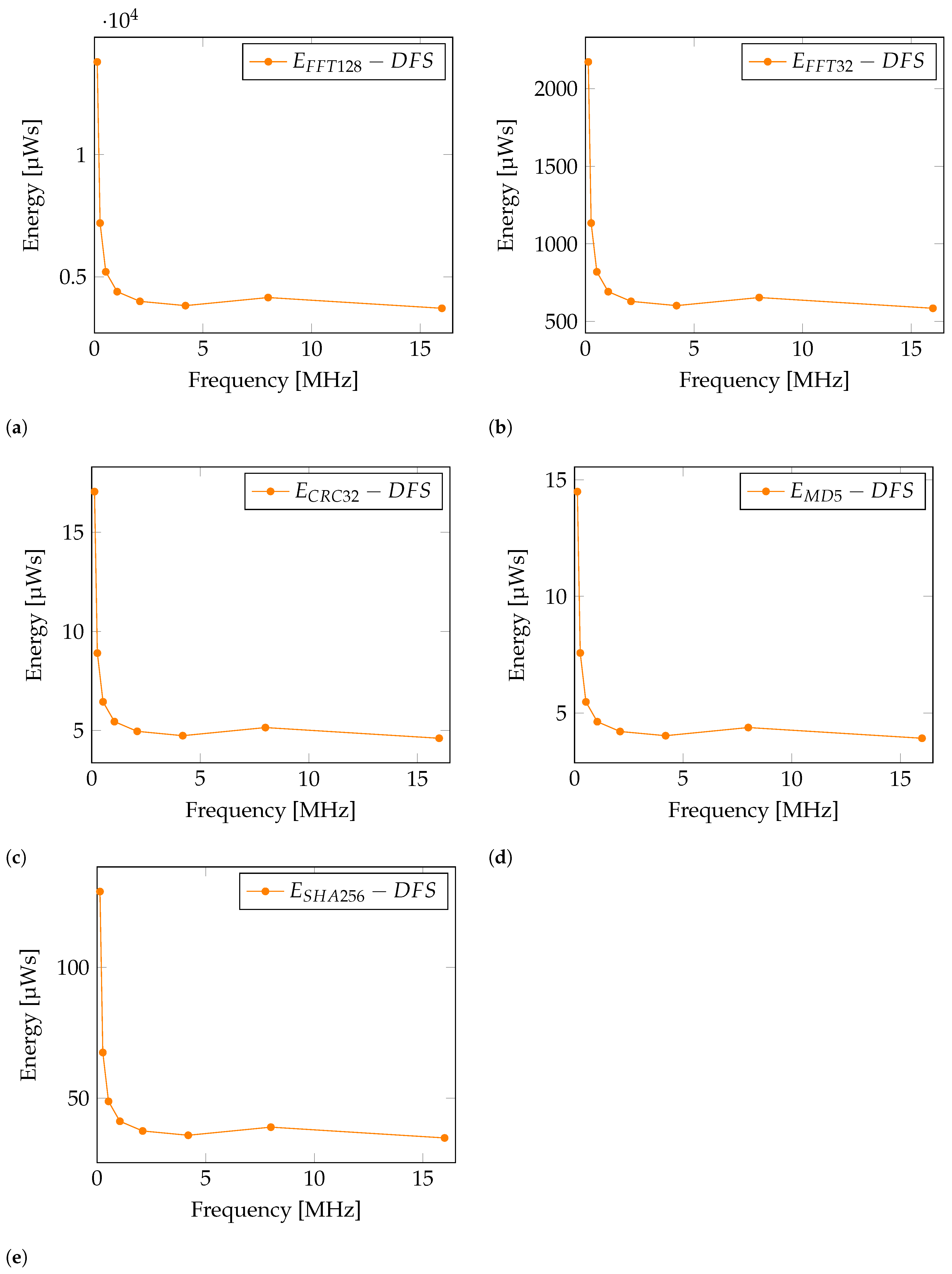
With the interpretation of results in Table 2, the presence of one anomaly is noticeable. Energy consumption results at a frequency of 8000 kHz is higher than expected, and can be seen in Figure 4. The reason for this is found in the configuration of the MCU. A phase-locked loop (PLL) is used only in this case, to achieve a frequency of 8000 kHz. Therefore, an increased energy consumption is caused by the operation of PLL.

Figure 4. Energy consumption graph with applied DFS for operation: (a) $E_{FFT128}$, (b) $E_{FFT32}$, (c) $E_{CRC32}$, (d) $E_{MD5}$, (e) $E_{SHA256}$.

3.3. Dynamic Voltage and Frequency Scaling

For additional energy savings, dynamic voltage scaling (DVS) is added to DFS. DVFS is a proven technique that further enhances battery life in portable devices and minimizes energy consumption in data centers [11,43]. When full performance is not required, voltage scaling can significantly reduce power consumption without impact on functionality. Voltage and frequency scaling are effective means to balance performance and power efficiency in various sorts of computing systems. Focus of this subsection is proposition of voltage values calculation, as insufficient operating voltage can impact the usability and stable operation of the microcontroller or microprocessor. Formula for voltage values calculation is:

$$U_{DVFS}\left(f\right)=A\times e^{f/B}\left[V\right],$$

(2)

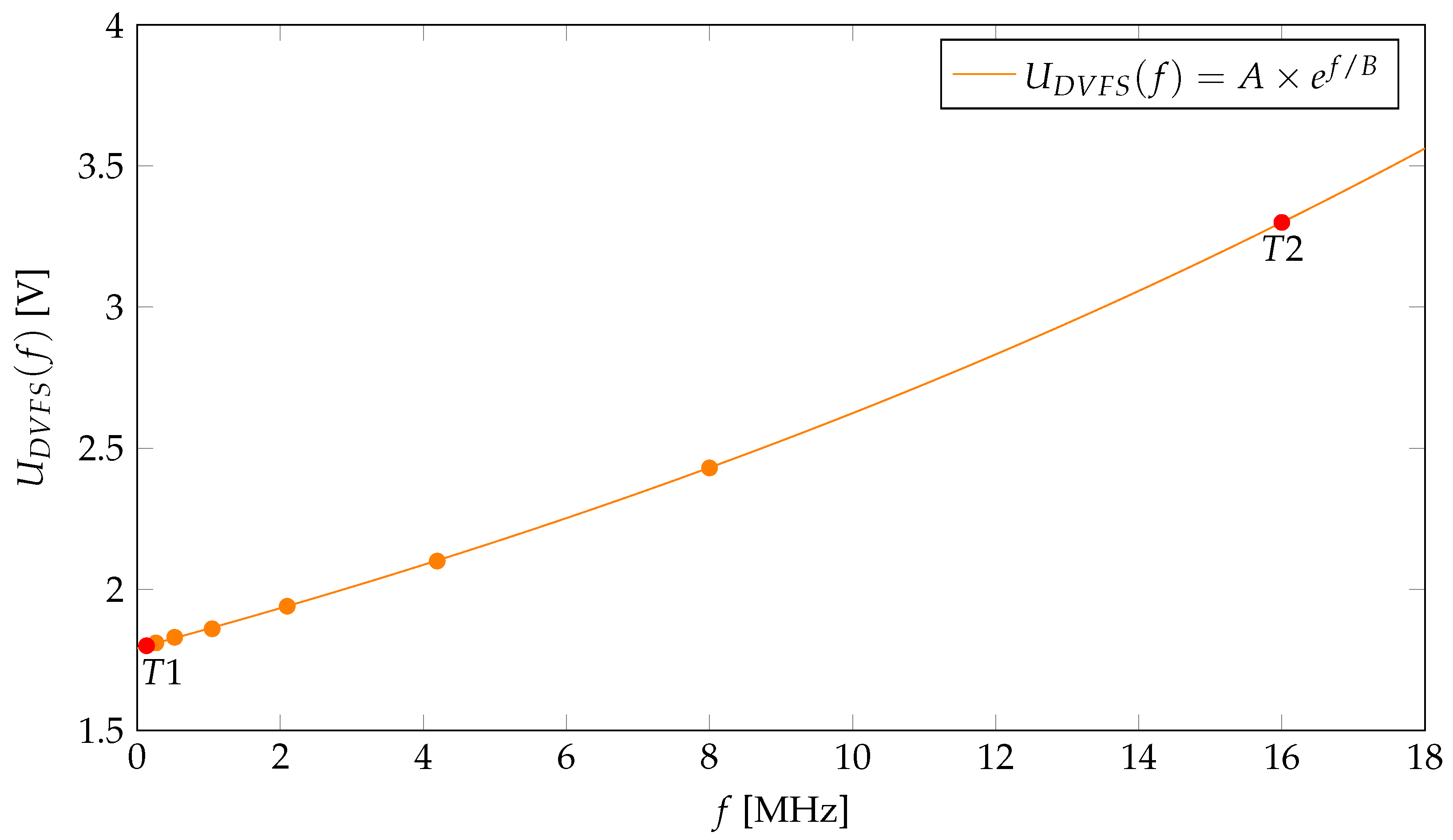
where $A=1.791011$ and $B=26.1804846$. $U_{DVFS}\left(f\right)$ is calculated based on the selected microcontroller power supply values and corresponding frequencies. Based on the MCU datasheet [38], the lowest power-supply value is $1.8$ V for the frequency $0.131$ MHz. In the same manner, for the frequency 16 MHz, the corresponding power-supply value is $3.3$ V. Hence, two points are established, T1 (0.131, 1.8) and T2 (16, 3.3). Regresion is used to calculate $U_{DVFS}\left(f\right)$ exponential function in Equation (2), based on the T1 and T2 points. Regression analysis was performed using Microsoft Excel 2019, as it provides the capability to execute linear and nonlinear regression models through its built-in functions and tools. The f-axis refers to operating frequencies in MHz, and the $U_{DVFS}\left(f\right)$-axis represents corresponding voltage values in volts, as shown in Figure 5.

Figure 5. Exponential model for stable voltage calculation (red circles mark points $T1$ and $T2$).

By inserting frequency values from Table 1 into Equation (2), corresponding voltage levels for each frequency can be calculated. Calculated voltage levels can be seen in Table 3 marked as $U_{DVFS}$. These values are representations of DC–DC converter targeted voltages during operation.

Table 3. Calculated energy consumption with dynamic voltage and frequency scaling (bold values mark the lowest energy consumption).

$\mathbf{f}\left[\mathbf{kHz}\right]$	${\mathbf{I}}_{\mathbf{DVFS}}\left[\mathbf{mA}\right]$	${\mathbf{U}}_{\mathbf{DVFS}}\left[\mathbf{V}\right]$	${\mathbf{E}}_{\mathbf{FFT}128}\left[\mathsf{\mu }\mathbf{Ws}\right]$	${\mathbf{E}}_{\mathbf{FFT}32}\left[\mathsf{\mu }\mathbf{Ws}\right]$	${\mathbf{E}}_{\mathbf{CRC}32}\left[\mathsf{\mu }\mathbf{Ws}\right]$	${\mathbf{E}}_{\mathbf{MD}5}\left[\mathsf{\mu }\mathbf{Ws}\right]$	${\mathbf{E}}_{\mathbf{SHA}256}\left[\mathsf{\mu }\mathbf{Ws}\right]$
131	0.05970	1.80	7411.90	1167.92	9.17	7.79	69.31
262	0.08679	1.81	3761.05	592.51	4.66	3.96	35.25
524	0.14471	1.83	2747.86	432.90	3.41	2.89	25.76
1048	0.26162	1.86	2376.75	374.42	2.95	2.50	22.28
2097	0.49866	1.94	2285.48	360.06	2.83	2.41	21.43
4194	0.97246	2.10	2378.58	374.70	2.95	2.51	22.30
8000	2.03865	2.43	3001.95	472.92	3.72	3.16	28.15
16,000	3.73185	3.30	3715.34	585.21	4.61	3.92	34.83

In order to implement dynamic voltage scaling, an efficiency assessment of the proposed solution is required. Inadequate efficiency may render DVS cost-ineffective, as it can increase production costs without delivering the expected benefits. Hence, a high level of efficiency is crucial for DVS to be a viable option. To effectively explore the relationship between DC–DC converter efficiency and DVS, it is essential to understand each concept independently. The efficiency of DC–DC converters, especially in the context of linear converters, has evolved significantly with technological advancements. Initially, with the introduction of switch-mode power supplies in the mid-1970s, DC–DC conversion efficiency improved significantly, from 60% to 80%, making them a popular solution in power supply systems [44]. With the goal of high efficiency across a range of voltages, modern DC–DC converters utilize adaptive control mechanisms. These systems adjust operating parameters in real-time to respond to the dynamic demands imposed by DVS. Consequently, DVS reduces DC–DC converter efficiency. Optimization of energy consumption in various electronic devices relies on the relationship between DVS and DC–DC converter efficiency.

Table 3 shows results of energy consumption per operation, but this time with applied DVFS. It can be noted that at 2097 kHz an optimal point has been reached for energy per operation. This suggests that the primary focus of energy-efficient design is geared towards optimizing under these conditions. Hence, newly designed system can benefit from operating voltage of 1.94 V and operating frequency of 2097 kHz, in case of ultra low power requirements. It is also worth mentioning that the DVFS execution times of the proposed operations in Table 1 remain unchanged, as the operating frequency is not affected.

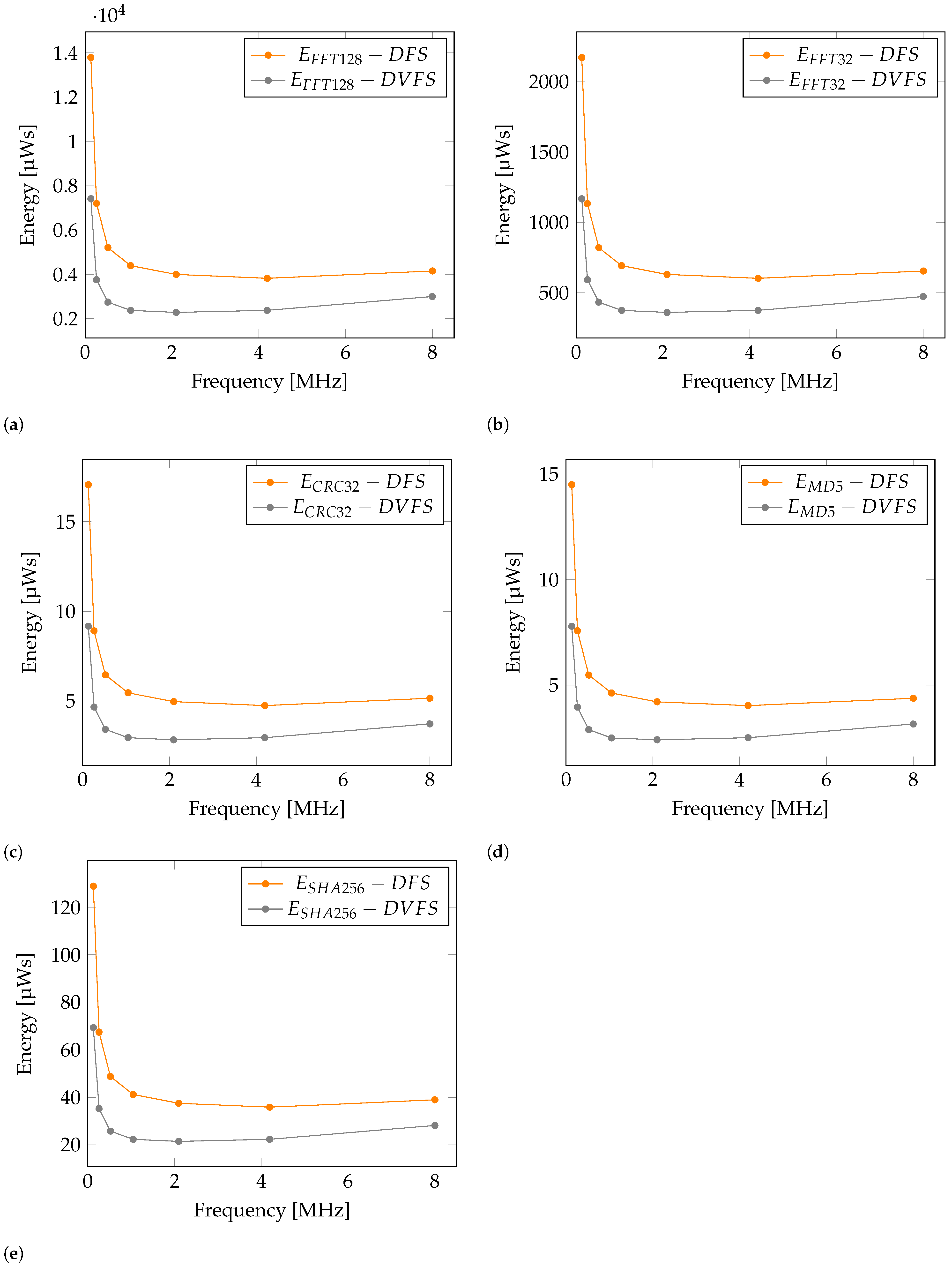
Figure 6 shows comparison between DFS and DVFS in terms of energy consumption for selected operations. Here it can be seen how reduced voltage can also significally impact energy consumption. Values at frequency of 16,000 kHz are not included, as there are no voltage difference between DFS and DVFS in this case. Furthermore, Energy reduction (ER) percentage is introduced as a measure of energy reduction between DFS and DVFS. Calculation formula is presented in Equation (3). Based on the formula, values in Table 4 are calculated. Results in Table 4 present Energy reduction per operation from 27.74% up to 47.74% in comparison with DFS values. It is visible that the highest energy savings are present at lower operating frequencies.

$$E{R}_{ALG}=\left(\frac{E_{ALG}^{DFS}-E_{ALG}^{DVFS}}{E_{ALG}^{DFS}}\right)\times 100[\%]$$

(3)

Figure 6. DVFS compared to DFS. Energy consumption graph for operation: (a) $E_{FFT128}$, (b) $E_{FFT32}$, (c) $E_{CRC32}$, (d) $E_{MD5}$, (e) $E_{SHA256}$.

Table 4. Calculated percentage of energy reduction for DFS vs. DVFS.

$\mathbf{f}\left[\mathbf{kHz}\right]$	${\mathbf{ER}}_{\mathbf{FFT}128}[\%]$	${\mathbf{ER}}_{\mathbf{FFT}32}[\%]$	${\mathbf{ER}}_{\mathbf{CRC}32}[\%]$	${\mathbf{ER}}_{\mathbf{MD}5}[\%]$	${\mathbf{ER}}_{\mathbf{SHA}256}[\%]$
131	46.23	46.23	46.23	46.23	46.23
262	47.74	47.74	47.74	47.74	47.74
524	47.20	47.20	47.20	47.20	47.20
1048	45.91	45.91	45.91	45.91	45.91
2097	42.84	42.84	42.84	42.84	42.84
4194	37.79	37.79	37.79	37.79	37.79
8000	27.74	27.74	27.74	27.74	27.74

3.4. Statistical Significance of the Results

Table 2 and Table 3 are combined and used in the statistical analysis of the energy consumption of selected operations. Table 2 has eight measurements with a change in frequency at a fixed voltage, while Table 3 has eight measurements with a change in frequency and voltage. The last row in both tables has the same frequency and voltage values. By removing this duplicate, the combined table has 15 rows of measured energy consumption values and is considered for various statistical tests.

The statistical analysis was conducted to provide insight into the statistical significance of the proposed results and to understand the differences in energy consumption among various selected operations. The paired t-test analysis was applied to all combinations of selected operations. The results shown in Table 5 reveal statistically significant differences, with the maximum p-value of 4.35 × ${10}^{-6}$. There is only one exception for the outlier pair $E_{CRC}$ and $E_{MD5}$ with a p-value of 0.382. This indicates significant variations in power consumption among selected operations, except for one outlier pair. The independent t-test between $E_{CRC}$ and $E_{MD5}$ also showed no statistically significant difference, indicating similar energy consumption between these algorithms. Wilcoxon test resulted in extremely low p-values for most pairs, with the maximum value of 0.000122. The statistic values are 0 for most pairs since all values in one group are greater than or equal to those in the other group. Therefore, there exists a strict difference in the distributions of energy consumption. The ANOVA test showed significant differences among the groups $E_{CRC}$, $E_{MD5}$, and $E_{SHA256}$ with a p-value of 0.0004, confirming variations in consumption.

Table 5. Statistical significance with t-test and Wilcoxon test.

Combination	t-Test p-Values	Wilcoxon p-Values
(EFFT128, EFFT32)	1.89 × ${10}^{-7}$	6.10 × ${10}^{-5}$
(EFFT128, ECRC)	2.52 × ${10}^{-7}$	6.10 × ${10}^{-5}$
(EFFT128, EMD5)	2.76 × ${10}^{-7}$	6.10 × ${10}^{-5}$
(EFFT128, ESHA256)	4.29 × ${10}^{-7}$	0.000122
(EFFT32, ECRC)	1.96 × ${10}^{-6}$	6.10 × ${10}^{-5}$
(EFFT32, EMD5)	4.35 × ${10}^{-6}$	0.000122
(EFFT32, ESHA256)	4.30 × ${10}^{-7}$	0.000122
(ECRC, EMD5)	0.382	0.008362
(ECRC, ESHA256)	4.21 × ${10}^{-7}$	0.000122
(EMD5, ESHA256)	4.21 × ${10}^{-7}$	0.000122

3.5. Energy Aware Embedded System Design

Energy-aware embedded system design includes the combination of both hardware and software to create energy aware system, in order to achieve more efficient and sustainable solutions. One of the key aspects of energy aware system design is PPW analysis, as it aims to meet performance requirements while minimizing energy usage. PPW in Table 6 is derived only from operating frequency, and measured current and voltage, but confirms the results obtained in Table 3.

Table 6. Calculated performance per watt values for energy aware system (higher is better).

$\mathbf{f}\left[\mathbf{kHz}\right]$	${\mathbf{I}}_{\mathbf{DVFS}}\left[\mathbf{mA}\right]$	${\mathbf{U}}_{\mathbf{DVFS}}\left[\mathbf{V}\right]$	$\mathbf{PPW}[\mathbf{kHz}/\mathbf{mW}]$
131	0.05970	1.80	1219.683
262	0.08679	1.81	1669.726
524	0.14471	1.83	1982.774
1048	0.26162	1.86	2148.801
2097	0.49866	1.94	2167.205
4194	0.97246	2.10	2051.563
8000	2.03865	2.43	1614.152
16,000	3.73185	3.30	1299.218

From the software development perspective, Algorithm 5 provides adequate individual approach to each load. In this instance Load1 is an example of time critical load, and High performance mode is selected as fastest option. Furthermore, Load2 is an example of light load which does not have real-time deadline, hence it can be performed in a power saving mode. Load3 is example of load with soft deadline, where the goal is to complete task with least energy possible. It is also worth mentioning that load_condition variable can become true in case of internal condition or external event. This consequently ensures operation of Power saving mode by default, until designated load condition occurs.

Algorithm 5 Programming model for dynamic frequency adjustment for per-load requirements

1: HAL init 2: Clock configuration ← Default(Power saving mode) 3: GPIO init 4: Initialize private variables 5: while 1 do 6:     if $load1\_condition$ is true then 7:         Load1 begin ← select mode(High performance mode) 8:         Load1 execute 9:         Load1 end ← select mode(Power saving mode) 10:     end if 11:     if $load2\_condition$ is true then 12:         Load2 begin 13:         Load2 execute                     ▹ Performs in power saving mode 14:         Load2 end 15:     end if 16:     if $load3\_condition$ is true then 17:         Load3 begin ← select mode(Energy efficient mode) 18:         Load3 execute 19:         Load3 end ← select mode(Power saving mode) 20:     end if 21: end while

The correct adjustment of voltage and frequency can further reduce energy consumption when performing specified operations in an embedded system. However, this does not always apply when very strict timing is involved. The transition from Power saving mode to High performance mode can cause delay which can introduce errors in tasks with strict timing constraints.

Depending on the device application, additional DC–DC converter can be added to enable DVS. In order to add adequate DC–DC converter, sufficient efficiency requirements should be met. However, in ultra-low-power applications there could be the case when there isn’t enough benefits with this additional development cost. In this case, it would be advisable to find and select the optimal point with the highest PPW value (Table 6).

4. Conclusions

The paper makes use of techniques such as dynamic frequency scaling and dynamic voltage scaling for improving energy efficiency of ultra-low-power devices. The paper also discusses an energy-saving approach that operates at the lowest frequency when computational demand is low, and scales up to optimal levels for maximum efficiency when higher computational power is needed. With this approach, system can automatically adapt energy levels in real time according to load requirements. Utilization of DFS leads to improvements in terms of energy consumption, in comparison to fixed operating frequency set by the program configuration. Additionally, results indicate that introducing DVS in combination with DFS can reduce energy consumption from 27.74% up to 47.74%. Furthermore, the results of the PPW analysis show the optimal operating point, which plays an important role in the design of energy aware system. In terms of statistical significance, it can be stated that low p-values, typically below 0.05, indicate a low likelihood that the observed differences between groups are the result of random variation.

The proposed approach for achieving ultra-low-power properties is implemented. When computational power is required, it is optimal to elevate the frequency to its maximum (in this instance, 16,000 kHz), execute the designated task, and then revert to the default operating frequency. When computational power is not requered, and the system is awaiting a specific event i.e., input from user, system condition or time event, the most efficient method to conserve energy during that timeframe is to operate at the lowest frequency (in this instance, 131 kHz). When energy is important factor, it is advisable to identify the optimal balance between performance and power consumption. Therefore, system can idle at minimum frequency when computational power is not needed, and boost to optimal values (in this case, 2097 kHz) to utilize energy in best possible way.

The long-term impact of DVFS is present in significant energy savings, as it allows devices to adjust voltage and operating frequency based on workload demands, thereby reducing total power consumption. Additionally, DVFS improves temperature management by reducing heat generation through lower power usage, which can increase device reliability and longevity. Although DFS has several advantages, certain disadvantages are also present. Performance impact and introduced latency are present. When transitioning from different frequency states, unpredictable performance can be caused in some cases. While DFS is intended to be energy efficient, this isn’t always the case. The effectivnes of DFS depends on the applied workload. Under certain conditions, constant switching between loads can consume more energy than running with fixed frequency. With addition of voltage scaling, DVFS can also introduce additional challenges. Mainly, rapid voltage changes can cause voltage drops which can result in unstable operation. Accurate and stable voltage regulation is needed combined with adequate energy efficiency. Finally, the challenges in this research are a good basis for future work in development of ultra-low-power embedded systems.