Computational Intelligence Supporting the Safe Control of Autonomous Multi-Objects

Abstract

The essence of this work, which is an extension of the author’s previous research, is an analysis of computational intelligence algorithms that the support safe control of an autonomous object moving in a large group of other autonomous objects. Linear and dynamic programming methods with neural constraints on the process state, as well as positional and matrix game methods, were used to synthesize computational algorithms for the safe trajectory of one’s own object. The aim of the comparative analysis of intelligent computational methods for the safe trajectory of an object was to show, through their use, the possibility of taking into account the risk of collision resulting from both the degree of cooperation of objects while observing traffic laws and the impact of the environment in the form of visibility and the complexity of the situation. Simulation tests of the algorithms were carried out on the example of a real navigation situation of several dozen objects passing each other at sea.

1. Introduction

Safely controlling large numbers of autonomous objects is a complex and demanding task that requires advanced design methods and technologies. Computational intelligence plays a significant role in solving this problem by enabling the implementation of effective object control algorithms. Thus, the following methods can be mentioned here: artificial neural networks, game control, fuzzy control, swarm intelligence, evolutionary programming, and multi-agent systems.

The development of the applications is presented in the following examples of computational intelligence methods for controlling various autonomous objects.

1.1. State of Knowledge

The analysis of the latest literature on the use of computational intelligence in the control of autonomous objects was carried out in the following way. First, works in the general scope of this topic were presented. Then, reference was made to works on specific types of autonomous objects: robots, land and aerial vehicles and ships.

In terms of the general topic of artificial intelligence control of autonomous objects, the following works can be mentioned.

In [1], Engel et al. present an intelligent control system for an autonomous object with a two-layer structure—a reflective layer and a reactive layer. The applied multi-agent adaptive fuzzy neural network combines low-level response with high-level reasoning and intelligent control.

Bathla et al. [2] have compared various autonomous vehicle solutions with artificial intelligence in the field of object detection, cybersecurity, and privacy. Autonomous trucks, buses, passenger cars, shuttles, helicopters, rovers, and subway vehicles were considered. The use of autonomous vehicles in supply chain management and the production process was planned.

In [3], Macrae deals with the analysis of the security of autonomous intelligent control systems in terms of sociotechnical sources of threat risk. For this purpose, five types of sociotechnical risk were formulated—structural, organizational, technological, epistemic, and cultural.

In [4], Tselentis et al. proposed the use of artificial intelligence methods to improve the traffic safety of road, railway, sea, and air facilities. For this purpose, they analyze statistical and econometric methods, algorithmic methods, classification and grouping, artificial neural networks, and optimization.

More and more work is being conducted on the use of artificial intelligence in robotics.

Xin in [5] improves the process of tracking multiple robots or vehicles in terms of improving precision and matching in the data association stage. They achieve this by calculating a tracking cost matrix that takes into account both the distance matrix and the position of moving targets and using a bidirectional recurrent neural network.

Razmjooei et al. [6] present a synthesis of finite-time sliding-mode position tracking control of a robot based on a time-varying perturbation observer.

Lee et al. [7] reduced the number of robot collisions by applying its training during the demonstration, thus obtaining a better support estimate to determine the policy of switching the robot away from the support boundary if it drifts close.

In [8], Azar and Koubaa propose the use of machine learning and deep learning artificial intelligence to build advanced robotics capable of performing many complex tasks and learning new challenges with better perception of the environment, which will lead to the implementation of control tasks with a response similar to that of human vision when detecting or recognizing other objects.

In [9], Soori et al. analyze the research and the increase in the efficiency of robots in land- and air-transport applications and assembly in production through the use of artificial intelligence, machine learning, and deep learning techniques.

However, most of the work concerns the use of artificial intelligence for autonomous vehicle control.

In [10], Schwarting et al. emphasize the great importance of machine learning in the integrated perception and planning of the movement of autonomous vehicles; in their work, they take into account the verification and safety of the control process.

In [11], Ma et al. analyze the use of artificial intelligence in the operation of autonomous vehicles in the fields of perception, location, mapping, and control. This use of artificial intelligence has resulted in high-resolution maps, big data, high-performance computing, and 5G communications.

In [12], Priyanka et al. characterize the role of artificial intelligence in the design of autonomous vehicles, with a particular emphasis on advanced sensor technology and control algorithms that are resistant to environmental changes.

In [13], Alabdulkreem et al. developed a computational intelligence algorithm for identifying and classifying such static and dynamic objects as pedestrians and vehicles, using the wild horse optimization method.

In [14], Naz et al. describe artificial intelligence algorithms for the perception, route planning, and traffic control of autonomous vehicles, with the aim of increasing their performance in complex environments.

In [15], Ming presents a fuzzy control algorithm for an autonomous vehicle along with a neural network algorithm for identifying changes in the immediate environment.

In [16], Sana et al. show that the use of machine learning and graphs in the synthesis of autonomous vehicle control ensures the safety of the vehicle’s movement in unfavorable weather conditions, intersections without signals, pedestrian crossings, roundabouts, and various situations in which there is a threat of collisions.

Elements of computational intelligence are also used in the field of maritime autonomous surface ship design.

In [17], Perera, taking into account the complex structure of the ship as a multi-level control system, envisages the use of agent systems with distributed intelligence at individual decision-making levels. The decision support layer uses a deep learning method to avoid ship collisions and takes into account the Convention on the International Regulations for the Prevention of Collisions at Sea (COLREG).

In [18], Martelli et al. present an intelligent autonomous ship traffic system, which consists of the following layers: the identification of the navigation situation and collision avoidance; the coordination of the movement of many ships, while taking into account environmental conditions; and the management of ship navigation in a crowded water area.

In [19], Veitch and Alsos point out that the effective consideration of human interaction with artificial intelligence requires significant interdisciplinary efforts with regard to the reconciliation of productivity with safety, the technical limitations related to human capabilities and expectations, and the autonomy of machine tasks with human control.

In [20], Guang et al. use the process of self-learning and continuous optimization to implement an intelligent control system for a maritime autonomous surface ship. The basis is the proximal policy optimization algorithm. The dynamics of an autonomous ship are described by the first-order nonlinear Nomoto model. However, the penalty function for exceeding the permissible distance between one ship and another ship or another obstacle was adopted as an index of control quality.

In [21], Johansen et al. used the assessment of a current collision risk combined with current information from the electronic navigation map to design an intelligent maritime autonomous surface ship control system. In this design, a Bayesian belief network was used as a risk model. The temporal logic method and Gaussian processes were used to verify compliance with the autonomous ship traffic safety requirements.

The most interesting works are those in the field of intelligent multi-object control. In [22], Yussupova et al. solve the problem of planning the routes of a group of objects, such as trains, in an unknown environment consisting of the many obstacles on a construction company site. A recursive algorithm was used to plan the path of the multi-connection manipulator.

In [23], Arnold et al. performed a computer simulation of a multi-object swarm algorithm of the control process of several dozen autonomous aerial robots that helped to locate victims during the occurrence of a flooded-building disaster.

In [24], Kotenko and Stankevitch analyze the implementation of the task of controlling the movement of a group of autonomous multi-objects, with particular emphasis on time constraints. The considerations were related to the following applications: virtual football, air combat operations, and computer hacker attacks.

In [25], Li et al. presented a multi-agent decision-making algorithm in air combat situations involving multiple unmanned aerial vehicles in a cooperative game; they used a decentralized, partially observable Markov decision process and a centrally learned distributed control system structure.

In [26], Muzahid et al. present an algorithm which plans the anti-collision strategy of multiple autonomous vehicles using a previously learned structure from an artificial neural network.

In [27], Dey and Xu developed a multi-agent cooperative mixed-game algorithm using distributed swarm control; the algorithm was supported by hierarchical learning. However, in order to consider the cooperation of the group leaders and their followers, the Stackelberg game model was used.

To sum up, the current literature does not present a comparison of the various computational intelligence methods for the safe control of large numbers of autonomous objects. Therefore, the aim of the article is first to present the algorithms: the neural network, position game, and risk game; then, a computer simulation of their operation using the example of a navigation situation involving the passing of several dozen objects is presented; finally, a comparative analysis is conducted with an optimization algorithm that does not use artificial intelligence.

1.2. Study Objectives

The research novelty of the work consists of the following:

• Synthesis of safe multi-object control algorithms in various degrees of object cooperation and environment complexity, using appropriately selected optimization methods, artificial intelligence, and game theory;
• Experimental comparative analysis of the effectiveness of methods using computational intelligence to determine the safe trajectories of many objects.

The results of the presented research will enable the use in practice of more effective multi-object control algorithms that take into account both the degree of cooperation between objects and the influence of the surrounding environment.

1.3. Article Content

First, the algorithms of safe multi-object control are presented. The next part presents the developed algorithms: optimal control, the artificial neural network, and the positional and risk games. Then, the results of the computer simulation of the computational intelligence algorithms are presented; this presentation allows for their comparative assessment with an algorithm without computational intelligence. The analysis of the research results and the scope of further research are included in the conclusions.

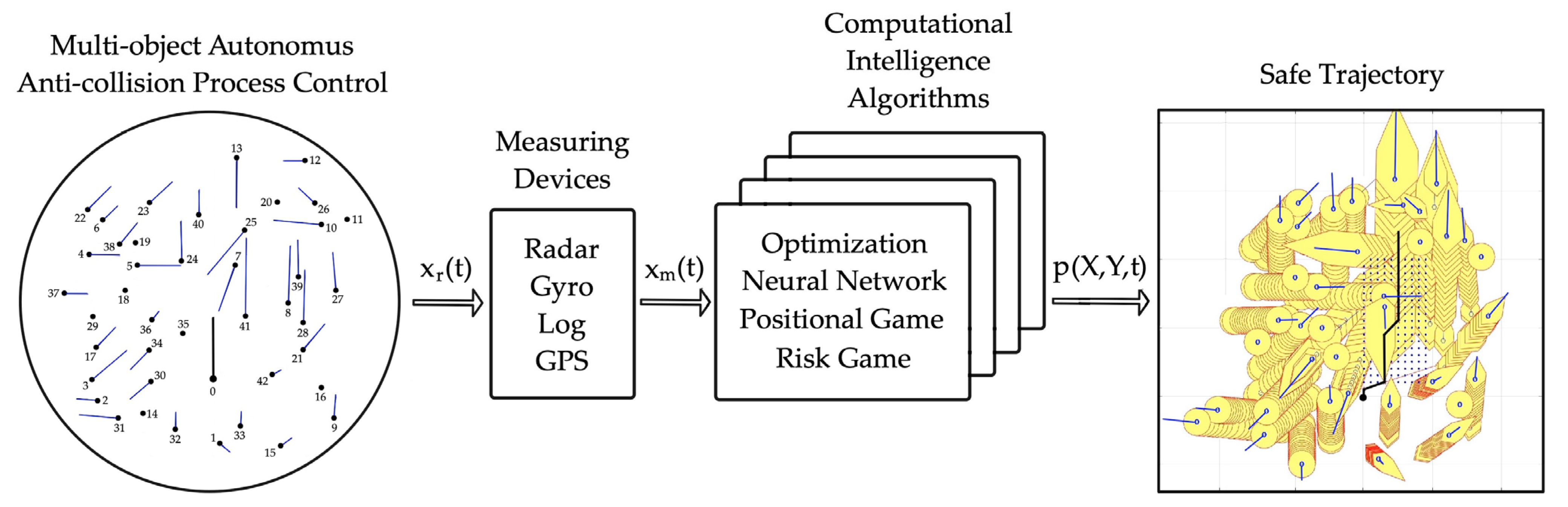
2. Algorithms of Safe Multi-Object Control

The system structure of safe multi-object control is considered, as shown in Figure 1. The current state of the multi-object autonomous anti-collision process control is monitored by measuring devices such as radar, gyro, log, and GPS.

The control process model is characterized by the simultaneous movement of many objects in an environment of variable visibility with a varying degree of cooperation between objects. These features of the control process can be taken into account by adapting the appropriate methods of computational intelligence in the form of optimization, artificial neural network, and game theory.

The essential part of the system comprises the computational intelligence algorithms for the safe trajectory of the object: a neural network with dynamic programming, a cooperative and non-cooperative positional game, and cooperative and non-cooperative risk games. For comparison purposes, an optimization algorithm without artificial intelligence was used.

The process model assumes a multi-step implementation of object control from the initial to the final state. The final state is determined by safely passing all the encountered objects and returning to the initial course.

The dynamics of the object are taken into account by taking the lead time of the course change maneuver as its adjustment time, which is approximately equal to the value of the three time constants of the object.

Individual algorithms differ in the way that they formulate the control objective function: from not taking into account changes in the courses and speeds of the encountered objects (OPT algorithm), through assigning domains generated by an artificial neural network (AI-NN algorithm) to the encountered objects, to taking into account the cooperative strategies of the encountered objects (AI-PGc and AI-Gc algorithms) as well as the non-cooperative strategies (AI-PGnc and AI-RGnc algorithms).

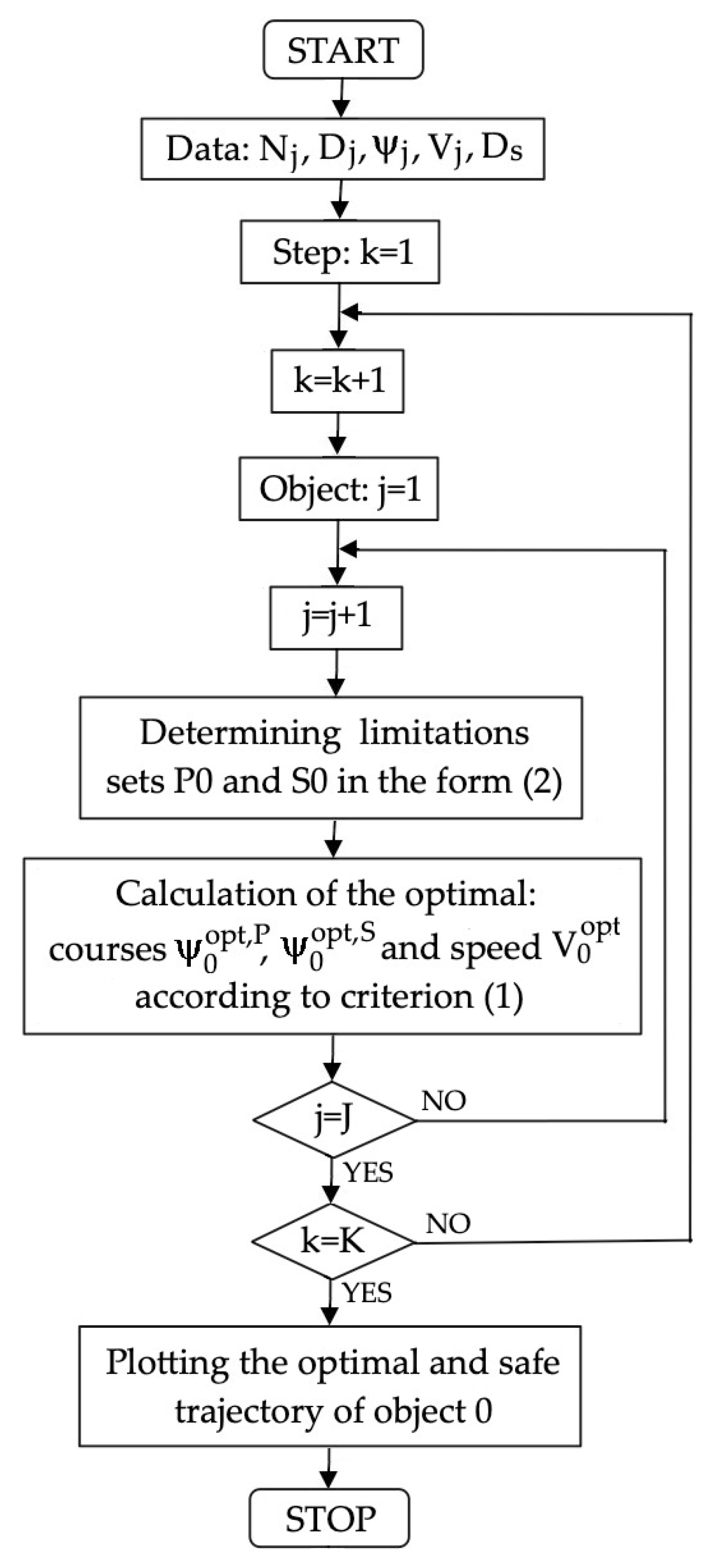
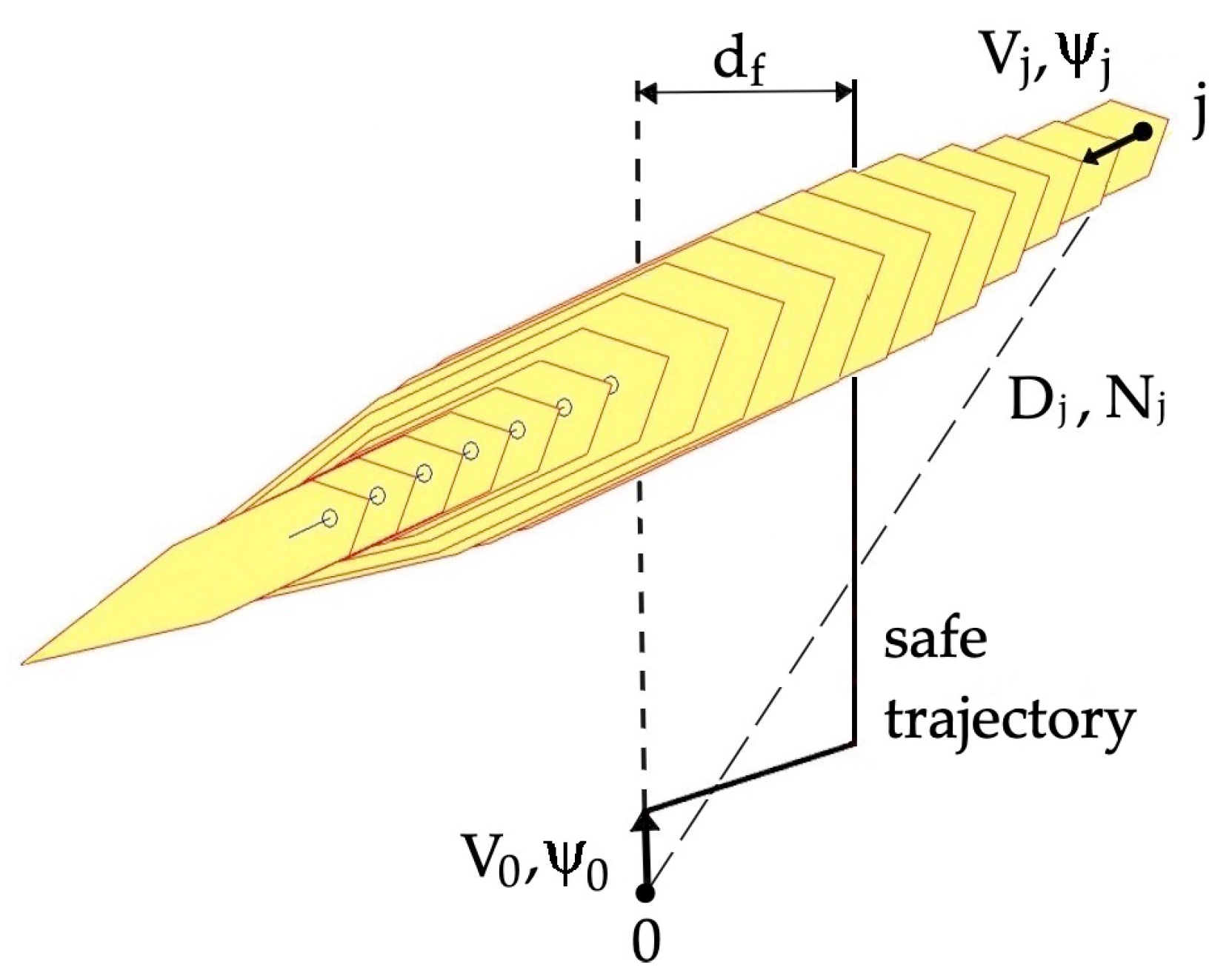
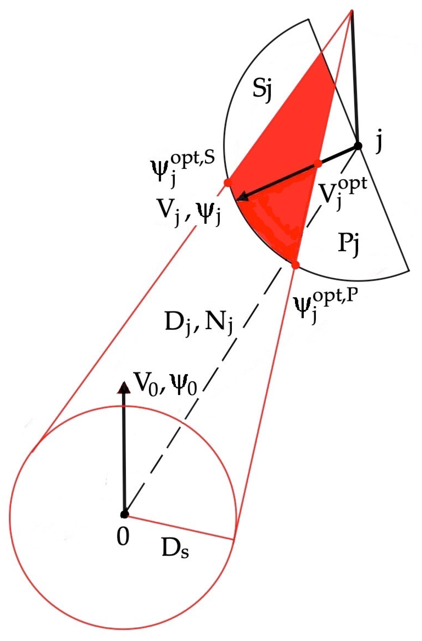
2.1. Algorithm of Optimal Control OPT

First, in order to assess the effects of the applied computational intelligence, the OPT optimal control algorithm was formulated as a reference; this reference did not contain elements of artificial intelligence.

It is assumed that the encountered objects j move with a constant course ψ_j and speed V_j. The basis for the synthesis of individual safe multi-object control algorithms involves first determining the sets of course and/or speed changes that ensure the safe passing of the objects; these sets are presented in Figure 2.

Object 0, moving with speed V₀ and course ψ₀ at a distance D_j and bearing N_j in relation to the encountered object j moving with speed V_j and course ψ_j, should pass it at a safe distance D_s. To achieve this, there are infinitely many possibilities of changing the course and speed from the set of permissible maneuvers to the port side of the P0 or to the starboard side of the S0; from this set, an optimal solution should be selected that ensures the maximum projection of the velocity vector in the given direction of movement of the object and leads to the smallest path losses during the safe avoidance of encountered objects [28].

The optimization criterion is the lowest path loss during the safe passing of all j objects; this is achieved with the maximum projection of the object’s velocity vector V₀ in the given direction x of its movement to the nearest turning point on the previously calculated path:

$$C_{OPT}=\underset{u_0\in \left(P0,S0\right)}{\max }{V}_{0x}\to \min s_0\to \min t_0$$

(1)

The minimum time criterion (1) leads to the achievement of a safe passing distance D_s, first by changing the course of object 0 to the value ${\psi }_0^{opt,P0}$ to the port side, or ${\psi }_0^{opt,S0}$ to the starboard side in a manner which adequately meets the requirements of the right of way. If this is not possible, the algorithm chooses to reduce the speed to the $V_0^{opt}$ value. Simplex linear programming is used to optimize this control task, which limits the possible solutions in the P0 and S0 linear sets:

$$a_{i}x+b_{i}y\le c_i i=1, \dots , I$$

(2)

finds the optimal solution to ensure the minimum control quality index (1).

In this way, the following OPT algorithm for the optimal control of object 0 in relation to a larger number of passing objects j is obtained, as in Figure 3, Algorithm 1.

Algorithm 1: Optimal Multi-Object Control Algorithm

BEGIN 1. Read Data: Nj, Dj, ψj, Vj, Ds 2. Step: k:=1 3. Object: j:=1 4. Determining limitations sets P0 and S0 in the form (2) 5. Calculation of the optimal: courses ${\mathsf{\psi }}_0^{opt,P}, {\mathsf{\psi }}_0^{opt,S}$ and speed   $V_0^{opt}$ according to criterion (1)   IF not j = J THEN (j:=j + 1 and GOTO 4)   ELSE k:=K   IF not  k = K THEN (k:=k + 1 and GOTO 3)   ELSE   Plotting the optimal and safe trajectory of object 0 END

2.2. Algorithm of Artificial Neural Network AI-NN

To consider the degree of danger of the movement of the passing objects j in each step k in the calculation of the safe trajectory of object 0, they are assigned a hexagonal domain, the size of which is shaped by a previously trained artificial neural network (Figure 4).

A neural network was used here to estimate the risk of a collision with object j. The estimate is a three-layer one-way artificial neural network with six neurons in the input layer, three neurons in the hidden layer, and one neuron in the output layer. The neurons in the input and hidden layers use a hyperbolic tangent activation function, and the output layer neuron has a sigmoidal unipolar activation function [29].

The determination of the optimal trajectory of object 0 from among the many possible safe trajectories that do not violate the moving neural areas of possible collisions with objects j is treated as a multi-stage decision-making process. The Bellman dynamic programming method was used to solve it, with a time-optimal optimization criterion:

$$C_{NN}^{AI}=\underset{u\in \left({\psi }_0,V_0\right)}{\min }C\left(x, u, t\right)\to \min t$$

(3)

In this way, the following artificial neural network AI-NN algorithm for the optimal and safe control of object 0 in relation to a larger number of passing objects j is obtained, as in Figure 5, Algorithm 2.

Algorithm 2: Artificial Neural Network Algorithm

BEGIN 1. Read Data: Nj, Dj, ψj, Vj, Ds 2. Step: k:=1 3. Object: j:=1 4. Determining the size of neural domain of object j   IF not j = J THEN (j:=j + 1 and GOTO 4)   ELSE Node: n:=1 6. Choosing the minimum-time of object 0 path in Bellman  dynamic programming   IF not n = N THEN (n:= n + 1 and GOTO 6)   ELSE k:=K   IF not  k = K THEN (k:=k + 1 and GOTO 3)   ELSE   Plotting the time-optimal and safe trajectory of object 0 END

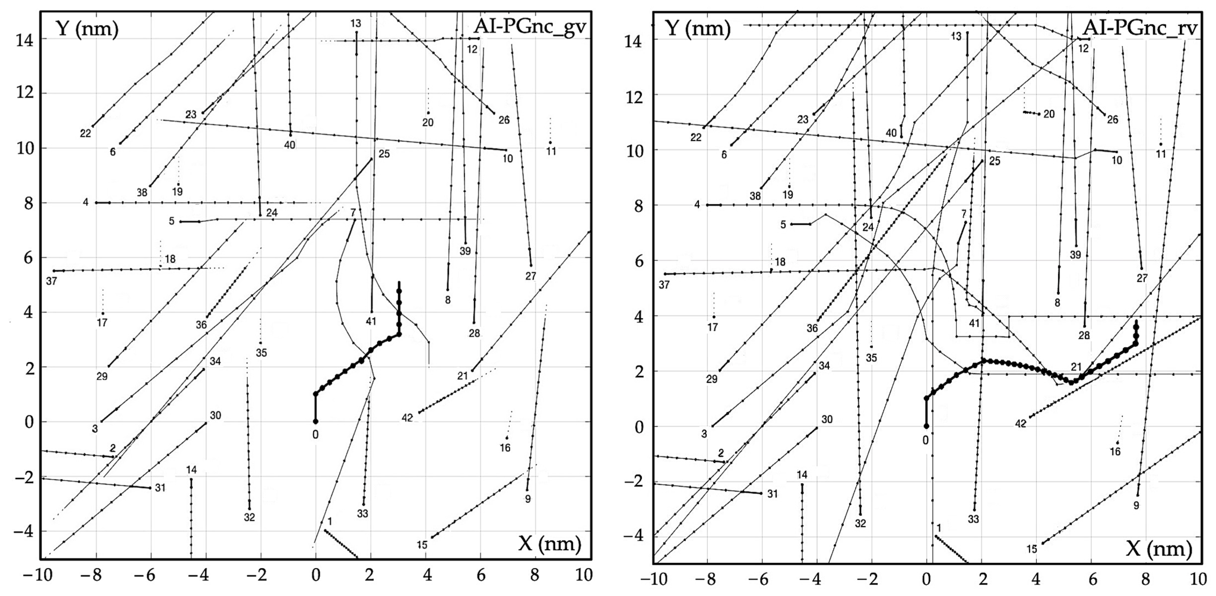
2.3. Algorithm of Positional Game AI-PG

In real navigation situations, objects may change course or speed to comply with the rules of the right of way, or they may act differently for various subjective reasons, which can lead to a collision. This creates a cooperative or non-cooperative game situation. If we transfer this process of object movement to the positions of objects, then we are dealing with a model of a multi-object positional game [30].

Then, for each object j, the sets of admissible strategies Pj and Sj to maintain the safe passing distance D_s are determined, as shown in Figure 6.

Object j moving with speed V_j and course ψ_j at distance D_j and bearing N_j in relation to object 0 may cooperate to avoid a collision or not cooperate; following a subjective error in the assessment of the situation, this can even lead to a collision.

For example, in the navigation situation shown in Figure 6, in the case of a cooperative game, object j will choose the course ψ_j^opt,S, while in a non-cooperative game it will choose the course ψ_j^opt,P.

Each computational step of the safe trajectory of object 0 consists of three stages:

• The determination of the optimal control of object 0 in relation to each object j ($\underset{u_0^j\in \left(P0,S0\right)}{\mathrm{m}\mathrm{a}\mathrm{x}}$);
• The determination of the optimal cooperative control (AI-PGc algorithm) or non-cooperative control (AI-PGnc algorithm) of individual objects j ($\underset{u_j\in \left(Pj,Sj\right)}{\mathrm{m}\mathrm{a}\mathrm{x}/\mathrm{m}\mathrm{i}\mathrm{n}}$);
• The determination of the optimal control of object 0 in relation to all objects j ($\underset{u_0\in \left(P0,S0\right)}{\mathrm{m}\mathrm{a}\mathrm{x}}$).

Then, the optimization criterion for object 0 in the cooperative position game will take the following form:

$$C_{PGc}^{AI}=\underset{u_0\in \left(P0,S0\right)}{\max }\underset{u_j\in \left(\mathit{Pj},\mathit{Sj}\right)}{\max }\underset{u_0^j\in \left(P0,S0\right)}{\max }{V}_{0x}\to \min s_0\to \min t_0$$

(4)

and in a non-cooperative game, it will take the following form:

$$C_{PGnc}^{AI}=\underset{u_0\in \left(P0,S0\right)}{\max }\underset{u_j\in \left(\mathit{Pj},\mathit{Sj}\right)}{\min }\underset{u_0^j\in \left(P0,S0\right)}{\max }{V}_{0x}\to \min s_0\to \min t_0$$

(5)

Then, an AI-PG positional game algorithm was developed to ensure optimal and safe control of object 0 in relation to a larger number of cooperative or non-cooperative j objects, as in Figure 7, Algorithm 3.

Algorithm 3: Positional Game Algorithm

BEGIN 1. Read Data: Nj, Dj, ψj, Vj, Ds 2. Step: k:=1 3. Object: j:=1 4. Determining optimal maneuvers of object 0: ${\mathsf{\psi }}_0^{opt,P}, {\mathsf{\psi }}_0^{opt,S},V_0^{opt}$   in relation to each object j 5. Triple programming 6. Algorithm AI-PGc max max max 7. Choosing cooperative maneuvers of object j: ${\mathsf{\psi }}_j^{opt,P}, {\mathsf{\psi }}_j^{opt,S},V_j^{opt}$ 8. Algorithm AI-PGnc max min max 9. Choosing non-cooperative maneuvers of object j: ${\mathsf{\psi }}_j^{opt,P}, {\mathsf{\psi }}_j^{opt,S},V_j^{opt}$   IF not j = J THEN (j:= j + 1 and GOTO 4)   ELSE Determining optimal maneuvers of object 0: ${\mathsf{\psi }}_0^{opt,P}, {\mathsf{\psi }}_0^{opt,S},V_0^{opt}$      in relation to each object j   IF not k = K THEN (k:= k + 1 and GOTO 3) ELSE Plotting the optimal and safe trajectory of object 0 END

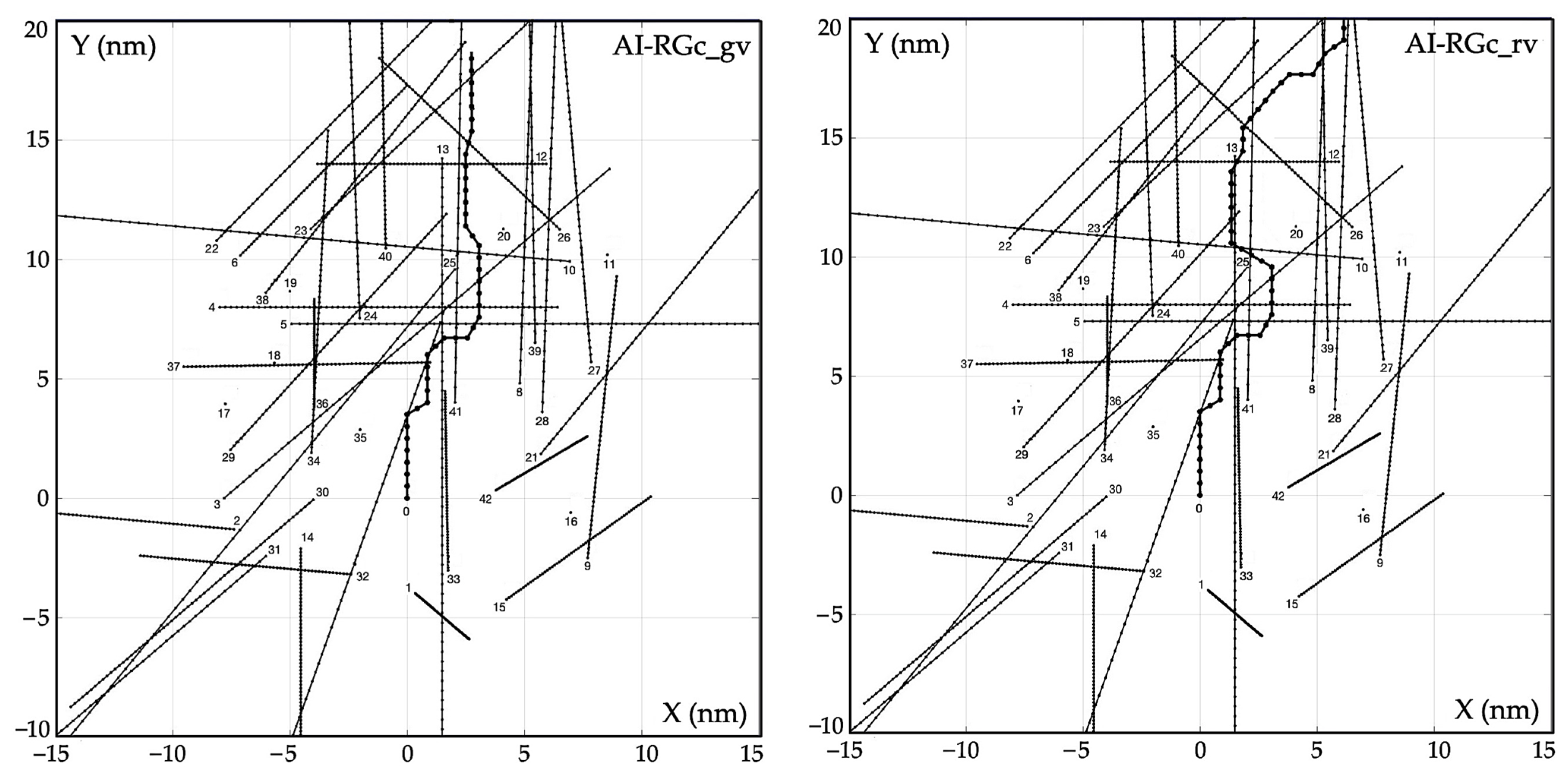
2.4. Algorithm of Risk Game AI-RG

Taking the risk of collision into account leads to the formulation of a multi-object matrix game model. The collision risk r_j is formulated as a function of the minimum distance D_j^min and time T_j^min until object j is passed by object 0 and the distance D_j between them:

$$r_j=f\left(D_j^{min}, T_j^{min}, D_j\right) 0\le r_j\le 1$$

(6)

In addition to the previously mentioned parameters of the objects’ proximity, the value of the collision risk depends primarily on their course and speed change maneuvers, i.e., the game control strategies (Figure 8).

A collision-risk matrix is formed, in which the number of rows corresponds to the number of maneuvering strategies of object 0, and the number of columns corresponds to the maneuvering strategies of individual objects j [31].

Thus, the optimization criterion in a cooperative matrix game will take the following form:

$$C_{RGc}^{AI}=\underset{u_0\in \left({\psi }_0,V_0\right)}{\min }\underset{u_j\in \left({\psi }_j,V_j\right)}{\min }{r}_j$$

(7)

and in a non-cooperative matrix game, the form is as follows:

$$C_{RGnc}^{AI}=\underset{u_0\in \left({\psi }_0,V_0\right)}{\min }\underset{u_j\in \left({\psi }_j,V_j\right)}{\max }{r}_j$$

(8)

The AI-RG algorithm for calculating the optimal and safe path of object 0 in relation to a larger number of cooperating or non-cooperating objects j is based on the matrix game model of the control process, as in Figure 9, Algorithm 4.

Algorithm 4: Risk Game Algorithm

BEGIN 1. Read Data: Nj, Dj, ψj, Vj, Ds 2. Step: k:=1 3. Object: j:=1 4. Calculation of optimal collision risk $r_j$    IF not j = J THEN (j:=j + 1 and GOTO 4) 6. Creation of collision risk matrix 7. Dual linear programming 9. Algorithm AI-RGc min min 10. Algorithm AI-RGnc min max   IF not  k = K THEN (k:= k + 1 and GOTO 3)   ELSE Plotting the optimal and safe trajectory of object 0 END

The algorithms presented above for the safe control of autonomous multi-objects are optimal OPT, neural network AI-NN, positional game AI-PG, and risk game AI-RG; they were implemented as computer programs in the MATLAB 2023 version software. In the current version, the programs have the ability to calculate the optimal path and the safe path of object 0 in relation to 100 other encountered objects.

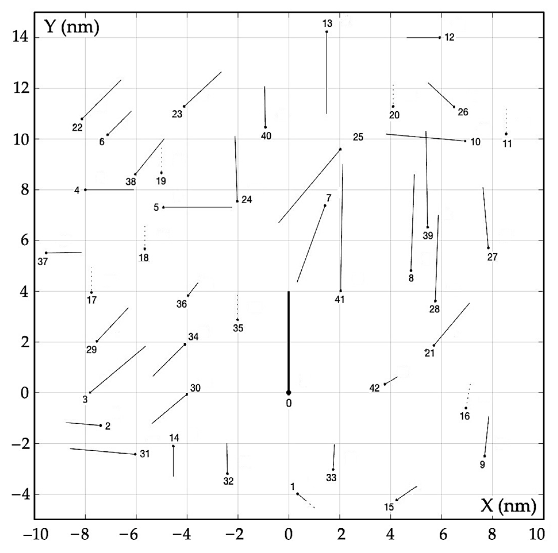
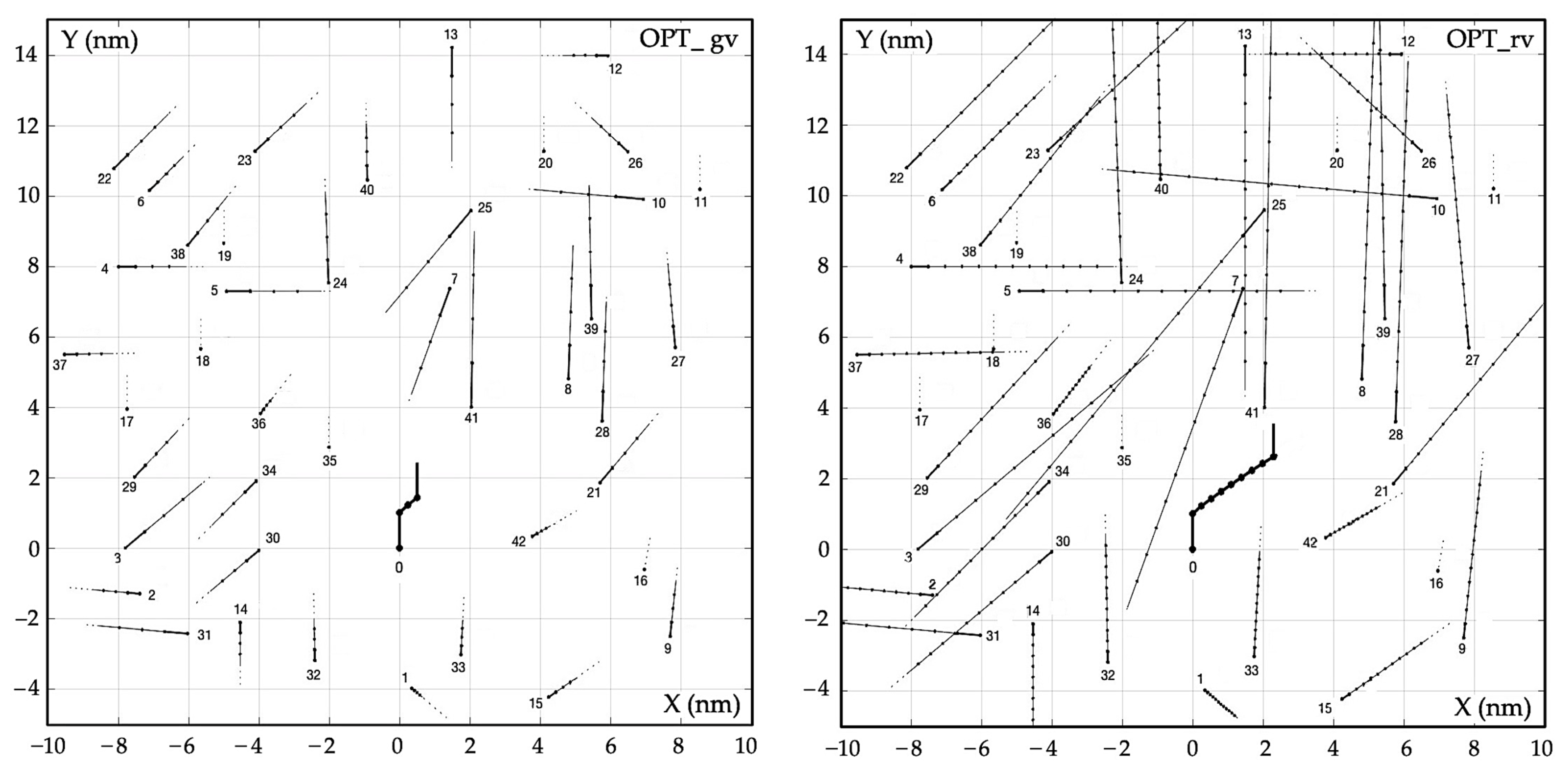
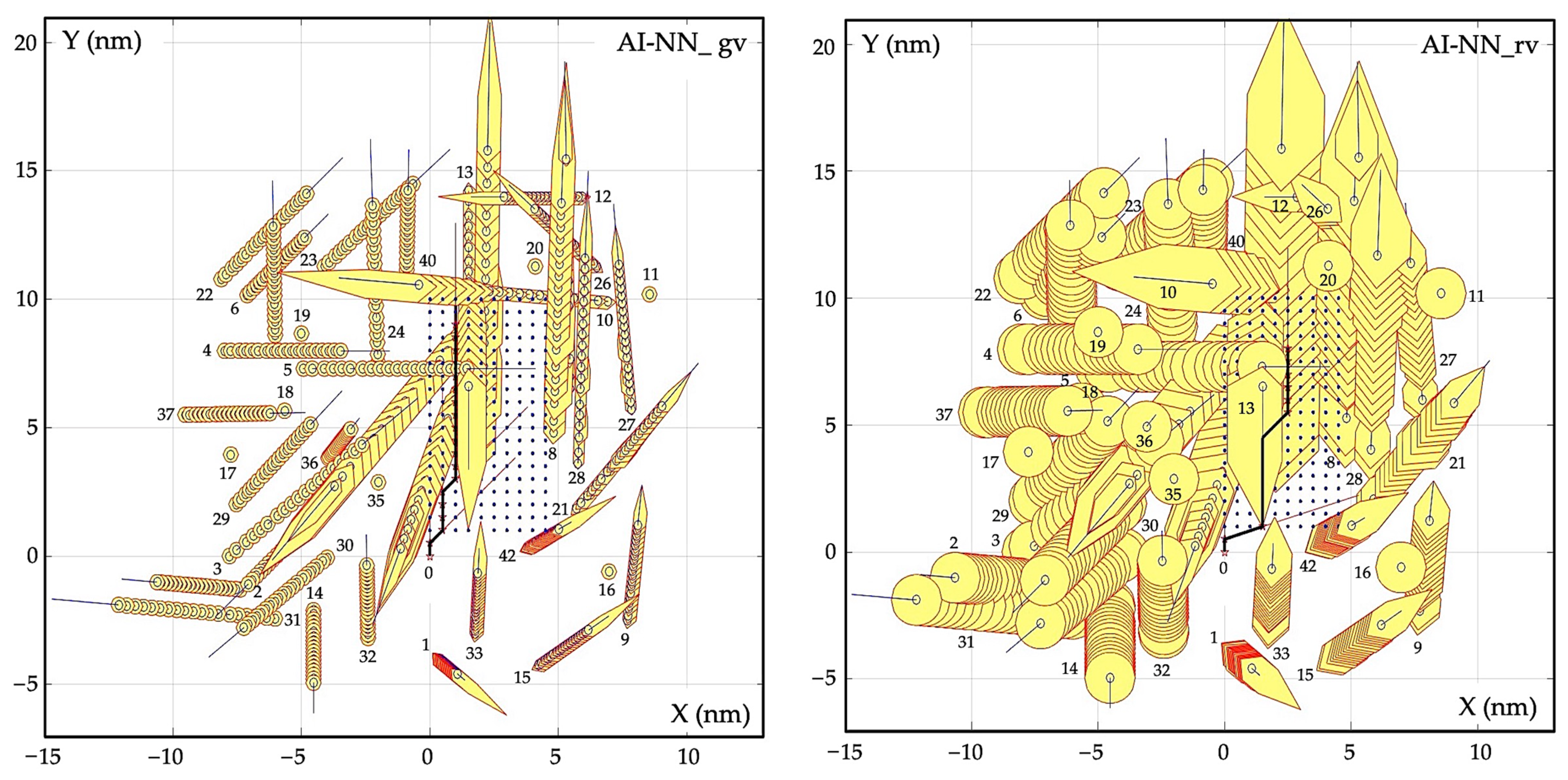
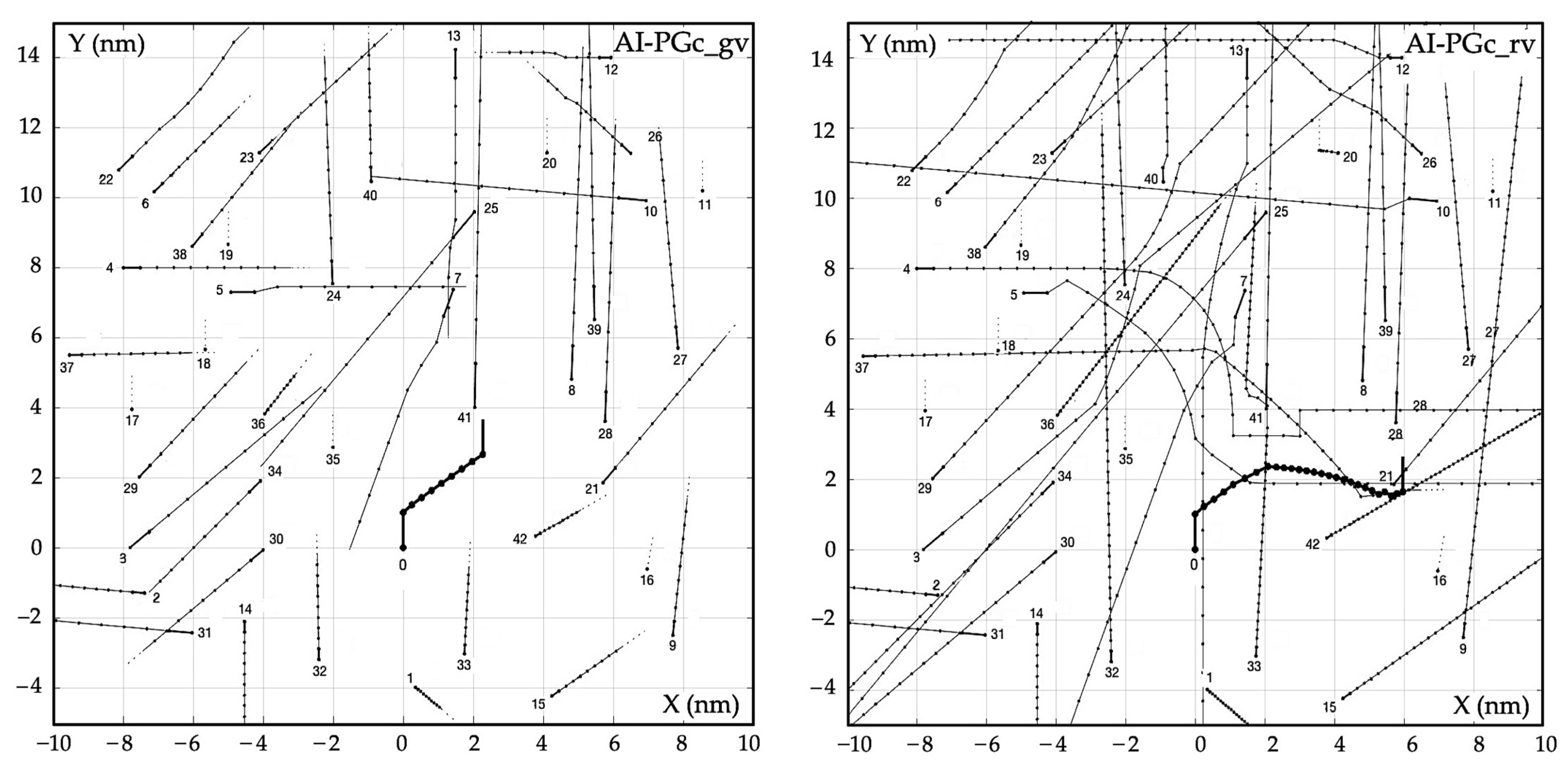
3. Experimental Comparative Analysis of Algorithms

The qualitative assessment of the individual computational intelligence algorithms AI-NN, AI-PG, and AI-RG was compared to the OPT algorithm without computational intelligence. The computer simulation was performed in MATLAB/Simulink 2023 version software. Data from the navigation situation recorded on a research and training vessel in the English Channel were used; in this situation, object 0 passed by 42 encountered objects. The data describing this situation are presented in

Table 1. Values, measured in the ARPA anti-collision system, of the state variables of the process of controlling the movement of object 0 and j = 42 passing objects.

Object j	Distance Dj (nm)	Bearing Nj (deg)	Speed Vj (kn)	Course ψj (deg)
0	-	-	20.0	0
1	4.0	175	2.0	130
2	7.5	260	6.9	275
3	7.8	270	14.3	50
4	11.3	315	9.6	90
5	8.8	326	13.5	90
6	12.4	325	6.7	45
7	7.5	11	16.0	200
8	8.8	45	19.0	2
9	8.1	108	7.9	6
10	12.1	35	15.7	275
11	13.3	40	0	0
12	15.2	23	6.5	270
13	14.3	6	16.2	180
14	5.0	245	6.0	180
15	6.0	135	5.0	55
16	7.0	95	0	0
17	8.7	297	0	0
18	8.0	315	0	0
19	10.0	330	0	0
20	12.0	20	0	0
21	6.0	72	11.0	40
22	13.5	323	11.0	45
23	12.0	340	10.0	47
24	7.8	345	13.0	358
25	9.8	12	19.0	220
26	13.0	30	7.0	313
27	9.7	54	12.0	355
28	6.8	58	17.0	2
29	7.8	285	9.0	43
30	4.0	269	9.0	230
31	6.5	248	13.0	275
32	4.0	217	6.0	359
33	3.5	150	5.0	3
34	4.5	295	9.0	225
35	3.5	325	0	0
36	5.5	314	3.0	38
37	11.0	300	7.0	89
38	10.5	325	9.0	39
39	8.5	40	19.0	359
40	10.5	355	8.0	359
41	4.5	27	25.0	1
42	3.8	85	3.0	60

.

The data were recorded in the Automatic Radar Plotting Aids (ARPA) anti-collision system and by the on-board log and gyrocompass.

The simulated navigation situation is depicted in Figure 10 in the form of twelve-minute velocity vectors of object 0 and passing objects j.

First, the algorithm OPT for determining the optimal path of object 0 was simulated without the use of computational intelligence (Figure 11), in conditions of good visibility (gv) and in conditions of restricted visibility (rv).

The advantage of the OPT method is the quick determination of a simple, safe object trajectory, while the disadvantage is that it does not take into account the maneuverability of other objects.

Then, the AI-NN algorithm for determining the optimal path of object 0 was simulated using computational intelligence in the form of an artificial neural network and Bellman dynamic programming (Figure 12) in conditions of good visibility (gv) and in conditions of restricted visibility (rv).

The advantage of the AI-NN method is that it takes into account the risk of collision when determining the safe trajectory of an object, while the disadvantage is that it does not take into account the possibility of maneuvering other objects.

A computer simulation of the cooperative and non-cooperative AI-GP positional game algorithm are presented in Figure 13 and Figure 14, respectively, in conditions of good and restricted visibility.

The advantage of the AI-PG method is that takes into account the possibility of cooperative and non-cooperative maneuvering of other objects, while the disadvantage is the longer computation time.

However, Figure 15 and Figure 16 show the results of the computer simulation of the AI-RG algorithm of the cooperative and non-cooperative matrix games, in conditions of good and restricted visibility.

The advantage of the AI-RG method is that it takes into account the possibility of cooperative and non-cooperative maneuvering of other objects, while the disadvantage is the more complicated course of the object’s safe trajectory.

The main task of the computational intelligence algorithms was to determine the optimal path of object 0 in order to ensure the safe passing of objects j. The optimization criterion included the integral component as the length of the path needed for object 0 to safely pass all objects j, with the final component being the final deviation d_f of the trajectory from the initial direction of movement.

The simulation tests of the algorithms within the full range of environmental impact, as represented by the safe passing distance D_s, allowed for the comparison of the algorithms containing various elements of artificial intelligence. As a result, the characteristics of the final deviation d_f of the safe path as a function of the safe distance D_s were obtained for the individual algorithms, which are presented in Figure 17.

A comparison of the computational intelligence algorithms AI-NN, AI-PG, and AI-RG was made with the OPT algorithm, which does not take into account either the subjective assessment of the situation involving approaching objects or the possible game nature of the process of passing objects. The use of the AI-RGnc and AI-PGnc algorithms takes into account the non-cooperative game course of the process of the safe passing of objects and leads to the largest deviation in the final path d_f, which is more than 4–5-times greater than the value for the OPT algorithm. However, the AI-RGc and AI-PGc cooperative game algorithms reduce the d_f deviation to 3-times the deviation of the OPT algorithm. The AI-RG risk game algorithm is 25% more sensitive than the AI-PG positional game algorithm. The algorithm AI-NN, which takes into account only the subjective assessment of the proximity of objects, has a final path d_f deviation that is 20% higher than that of the OPT algorithm.

4. Conclusions

The conducted synthesis of computational intelligence algorithms that support safe control in situations in which many autonomous objects are passed allows for the following final conclusions:

• The object-domain neural network model supported by dynamic programming allows for the elements of the subjective assessment of the navigation situation to be taken into account;
• The positional game model supported by triple linear programming enables the cooperative and non-cooperative safe control of a group of many encountered objects;
• The collision-risk matrix game model is supported by dual linear programming and provides a solution to the problem of safe multi-object cooperative and non-cooperative control.

The computer simulation of computational intelligence algorithms enabled their comparative assessment with the following scope:

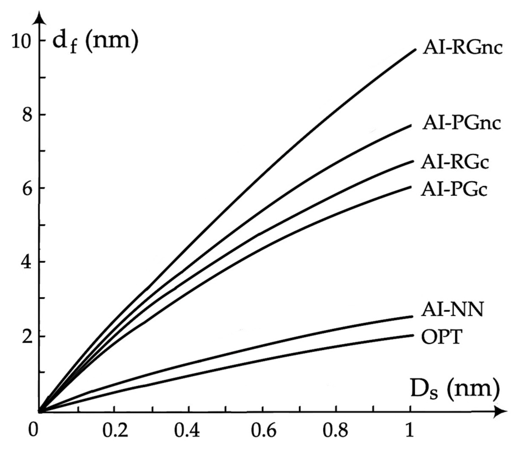
• The use of cooperative game algorithms reduces the final path deviation from 10 to 30% compared to non-cooperative game algorithms;
• The use of an artificial neural network in the AI-NN algorithm allows for an adequate representation of subjectivity in the assessment of the navigation situation, resulting in an increase in the final path deviation by only 10% compared to the OPT algorithm without artificial intelligence elements;
• In the situation in which object 0 passed only one object 1, the characteristics of the final path d_f deviation of the AI-RGc and AI-PGc algorithms would be below the characteristics of the NN and OPT algorithms due to the lack of other objects interacting with each other and indirectly with object 0.

The assessment of the empirical validation of safe control of autonomous multi-objects consists of:

• Use of real situation data from radar, log, and gyrocompass;
• Adequate selection of simulation parameters in the form of the values of the safe passing distance and the maneuver advance time needed for calculations and making a maneuvering decision.

The value of the final deviation of the object’s safe trajectory from its initial value was used as a metric for the comparative assessment of individual computational intelligence algorithms.

Further research on the use of computational intelligence methods to improve multi-objective control algorithms should proceed in the following directions:

• To take into account the uncertainty of the process model, the fuzzy-neural control method can be used;
• In order to achieve lower computational complexity, the use of particle swarm methods can be considered, for example in the form of the ant algorithm;
• In order to adapt to the real tasks of navigation of objects moving in unrestricted and restricted areas, it is necessary to provide the determination of a safe trajectory with the final condition in the form of a given final position or a given final course.

References

1. Engel, E.A.; Kovalev, I.V.; Engel, N.E.; Brezitskaya, V.V.; Prohorovich, G.A. Intelligent control system of autonomous objects. In Proceedings of the IOP Conference Series: Materials Science and Engineering, V International Workshop on Mathematical Models and their Applications, Krasnoyarsk, Russia, 7–9 November 2016; Volume 173. [Google Scholar]
2. Bathla, G.; Bhadane, K.; Singh, R.K.; Kumar, R.; Aluvalu, R.; Krishnamurthi, R.; Kumar, A.; Thakur, R.N.; Basheer, S. Autonomous Vehicles and Intelligent Automation: Applications, Challenges and Opportunities. Hindawi Mob. Inf. Syst. 2022, 2022, 7632892. [Google Scholar] [CrossRef]
3. Macrae, C. Learning from the Failure of Autonomous and Intelligent Systems: Accidents, Safety, and Sociotechnical Sources of Risk. Risk Anal. 2022, 42, 1893–2124. [Google Scholar] [CrossRef] [PubMed]
4. Tselentis, D.I.; Papadimitriou, E.; Gelder, P. The usefulness of artificial intelligence for safety assessment of different transport modes. Accid. Anal. Prev. 2023, 186, 107034. [Google Scholar] [CrossRef] [PubMed]
5. Xin, P. Multi-Objects Tracking Based on 3D Lidar and Bi-Directional Recurrent Neural Networks under Autonomous Driving. Ph.D. Thesis, School of Graduate Studies Electronic, Rutgers University, New Brunswick, NJ, USA, 18 January 2020. [Google Scholar] [CrossRef]
6. Razmjooei, H.; Shafiei, M.H.; Palli, G.; Arefi, M.M. Non-linear Finite-Time Tracking Control of Uncertain Robotic Manipulators Using Time-Varying Disturbance Observer-Based Sliding Mode Method. J. Intell. Robot. Syst. 2022, 104, 36. [Google Scholar] [CrossRef]
7. Lee, J.; Laskey, M.; Fox, R.; Goldberg, K. Constraint Estimation and Derivative-Free Recovery for Robot Learning from Demonstrations. arXiv 2018, arXiv:1801.10321. [Google Scholar]
8. Azar, A.T.; Koubaa, A. Artificial Intelligence for Robotics and Autonomous Systems Applications, 1st ed.; Springer: Berlin/Heidelberg, Germany, 2023; ISBN 978-3031287145. [Google Scholar]
9. Soori, M.; Arezoo, B.; Dastres, R. Artificial intelligence, machine learning and deep learning in advanced robotics, a review. Cogn. Robot. 2023, 3, 54–70. [Google Scholar] [CrossRef]
10. Schwarting, W.; Alonso-Mora, J.; Rus, D. Planning and Decision-Making for Autonomous Vehicles. Annu. Rev. Control. Robot. Auton. Syst. 2018, 1, 187–210. [Google Scholar] [CrossRef]
11. Ma, Y.; Wang, Z.; Yang, H.; Yang, L. Artificial intelligence applications in the development of autonomous vehicles: A survey. IEEE/CAA J. Autom. Sin. 2020, 7, 315–329. [Google Scholar] [CrossRef]
12. Priyanka, G.; Rajanika, D.; Dharavi, C.; Lakshika, B.; Neha, B. Role of Artificial Intelligence in Autonomous Vehicle. In Proceedings of the International Conference on Innovative Computing & Communication (ICICC), Delhi, India, 20–21 February 2021. [Google Scholar]
13. Alabdulkreem, E.; Alzahrani, J.S.; Nemri, N.; Alharbi, O.; Mohamed, A.; Marzouk, R.; Hilal, A.M. Computational Intelligence with Wild Horse Optimization Based Object Recognition and Classification Model for Autonomous Driving Systems. Appl. Sci. 2022, 12, 6249. [Google Scholar] [CrossRef]
14. Naz, N.; Ehsan, M.K.; Amirzada, M.R.; Ali, M.Y.; Qureshi, M.A. Intelligence of Autonomous Vehicles: A Concise Revisit. J. Sens. 2022, 2022, 2690164. [Google Scholar] [CrossRef]
15. Ming, G. Exploration of the intelligent control system of autonomous vehicles based on edge computing. PLoS ONE 2023, 18, e0281294. [Google Scholar] [CrossRef]
16. Sana, F.; Azad, N.L.; Raahemifar, K. Autonomous Vehicle Decision-Making and Control in Complex and Unconventional Scenarios—A Review. Machines 2023, 11, 676. [Google Scholar] [CrossRef]
17. Perera, L.P. Autonomous Ship Navigation Under Deep Learning and the Challenges in COLREGs. In Proceedings of the 37th International Conference on Ocean, Offshore and Arctic Engineering, Madrid, Spain, 17–22 June 2018. [Google Scholar]
18. Martelli, M.; Virdis, A.; Gotta, A.; Cassarà, P.; Di Summa, M. An Outlook on the Future Marine Traffic Management System for Autonomous Ships. IEEE Access 2021, 9, 157316–157328. [Google Scholar] [CrossRef]
19. Veitch, E.; Alsos, O.A. A systematic review of human-AI interaction in autonomous ship systems. Saf. Sci. 2022, 152, 105778. [Google Scholar] [CrossRef]
20. Guan, W.; Cui, Z.; Zhang, X. Intelligent Smart Marine Autonomous Surface Ship Decision System Based on Improved PPO Algorithm. Sensors 2022, 22, 5732. [Google Scholar] [CrossRef]
21. Johansen, T.; Blindheim, S.; Torben, T.R.; Utne, I.B.; Johansen, T.A.; Sørensen, A.J. Development and testing of a risk-based control system for autonomous ships. Reliab. Eng. Syst. Saf. 2023, 234, 109195. [Google Scholar] [CrossRef]
22. Yussupova, N.I.; Gonchar, L.E.; Rembold, U. Path Planning Algorithm of a Lot of Mobil Autonomous Objects in Unknown Constrained Environment. In Proceedings of the ISARC’99 International Symposium on Automation and Robotics in Construction, Madrid, Spain, 22–24 September 1999; pp. 403–407. [Google Scholar] [CrossRef]
23. Arnold, R.D.; Yamaguchi, H.; Tanaka, T. Search and rescue with autonomous flying robots through behavior-based cooperative intelligence. Int. J. Humanit. Action 2018, 3, 18. [Google Scholar] [CrossRef]
24. Kotenko, I.; Stankevitch, L. The control of teams of autonomous objects in the time-constrained environments. In Proceedings of the 2002 IEEE International Conference on Artificial Intelligence Systems (ICAIS 2002), Divnomorskoe, Russia, 5–10 September 2002; pp. 158–163. [Google Scholar] [CrossRef]
25. Li, S.; Wang, Y.; Zhou, Y.; Jia, Y.; Shi, H.; Yang, F.; Zhang, C. Multi-UAV Cooperative Air Combat Decision-Making Based on Multi-Agent Double-Soft Actor-Critic. Aerospace 2023, 10, 574. [Google Scholar] [CrossRef]
26. Muzahid, A.J.M.; Kamarulzaman, S.F.; Rahman, M.A.; Murad, S.A.; Kamal, M.A.S.; Alenezi, A.H. Multiple vehicle cooperation and collision avoidance in automated vehicles: Survey and an AI-enabled conceptual framework. Sci. Rep. 2023, 13, 603. [Google Scholar] [CrossRef] [PubMed]
27. Dey, S.; Xu, H. Intelligent Distributed Swarm Control for Large-Scale Multi-UAV Systems: A Hierarchical Learning Approach. Electronics 2023, 12, 89. [Google Scholar] [CrossRef]
28. Thie, P.R.; Keough, G.E. An Introduction to Linear Programming and Game Theory; Wiley: Hoboken, NJ, USA, 2008; ISBN 978-0-470-23286-6. [Google Scholar]
29. Lew, A.; Mauch, H. Dynamic Programming—A Computational Tool; Springer: Berlin/Heidelberg, Germany, 2007; ISBN 978-3-540-37014-7. [Google Scholar]
30. Faigle, U. Mathematical Game Theory, 1st ed.; World Scientific: Singapore, 2022; ISBN 978-981-1246-70-8. [Google Scholar]
31. Nisan, N.; Roughgarden, T.; Tardos, E.; Vazirani, V. Algorithmic Game Theory; Cambridge University Press: Cambridge, UK, 2007; ISBN 978-0-521-87282-9. [Google Scholar]
Figure 1. Computational intelligence algorithms in a multi-object anti-collision control system: xr(t) are real state variables; xm(t) are measured state variables; p(X,Y,t) is the optimal and safe object trajectory.
Electronics 13 00780 g001
Figure 2. Determining the set P0 with a change in course to the port side and set S0 with a change in course to the starboard side or a reduction in speed of object 0 to maintain a safe passing distance Ds from object j.
Electronics 13 00780 g002
Figure 3. Diagram of OPT optimal multi-object control.
Electronics 13 00780 g003
Figure 4. Illustration of the dangerous approach area of objects 0 and j in the form of a neural hexagonal domain: df is the final deviation of object 0 safe trajectory from the given direction of movement.
Electronics 13 00780 g004
Figure 5. Diagram of AI-NN artificial neural network optimal control.
Electronics 13 00780 g005
Figure 6. Determining the set Pj with a change in course to the port side and the set Sj with a change in course to the starboard side or a reduction in speed of object j to maintain a safe passing distance Ds from object 0.
Electronics 13 00780 g006
Figure 7. Diagram of AI-NPG positional game control.
Electronics 13 00780 g007
Figure 8. Maneuvering strategies (ψ0, V0) of object 0 and (ψj, Vj) of object j in the matrix game.
Electronics 13 00780 g008
Figure 9. Diagram of AI-RG risk game control.
Electronics 13 00780 g009
Figure 10. Illustration of the navigational situation of the object’s movement in relation to 42 other objects passed in the form of twelve-minute velocity vectors.
Electronics 13 00780 g010
Figure 11. The optimal trajectories of the object 0, without artificial intelligence, during safe passing of 42 other encountered objects j: (OPT_gv) in good visibility, when Ds = 0.3 nm; (OPT_rv) in restricted visibility, when Ds = 1 nm.
Electronics 13 00780 g011
Figure 12. Optimal object 0 trajectories, using an artificial neural network, while safely passing 42 other encountered objects j: (AI-NN_gv) in good visibility, when Ds = 0.3 nm; (AI-NN_rv) in restricted visibility, when Ds = 1 nm.
Electronics 13 00780 g012
Figure 13. Optimal object 0 trajectories, using a cooperative positional game, while safely passing 42 other encountered objects j: (AI-PGc_gv) in good visibility, when Ds = 0.3 nm; (AI-PGc_rv) in restricted visibility, when Ds = 1 nm.
Electronics 13 00780 g013
Figure 14. Optimal object 0 trajectories, using a non-cooperative positional game, while safely passing 42 other encountered objects j: (AI-PGnc_gv) in good visibility, when Ds = 0.3 nm; (AI-PGnc_rv) in restricted visibility, when Ds = 1 nm.
Electronics 13 00780 g014
Figure 15. Optimal object 0 trajectories, using a cooperative risk game, while safely passing 42 other encountered objects: (AI-RGc_gv) in good visibility, when Ds = 0.3 nm; (AI-RGc_rv) in restricted visibility, when Ds = 1 nm.
Electronics 13 00780 g015
Figure 16. Optimal object 0 trajectories, using a cooperative risk game, while safely passing 42 other encountered objects: (AI-RGnc_gv) in good visibility, when Ds = 0.3 nm; (AI-RGnc_rv) in restricted visibility, when Ds = 1 nm.
Electronics 13 00780 g016
Figure 17. Dependence of the final deviation df of object safe trajectory as function of the safe distance Ds of passing objects for AI algorithms: OPT optimal without AI; AI-NN neural network; AI-PGc cooperative positional game; AI-PGnc non-cooperative positional game; AI-RGc cooperative risk game; AI-RGnc non-cooperative risk game.
Electronics 13 00780 g017