Article

Sum Rate Optimization for Multi-IRS-Aided Multi-BS Communication System Based on Multi-Agent

School of Information and Electronics Engineering, Beijing Institute of Technology, Beijing 100081, China
*
Author to whom correspondence should be addressed.
Electronics 2024, 13(4), 735; https://doi.org/10.3390/electronics13040735
Submission received: 29 December 2023 / Revised: 6 February 2024 / Accepted: 8 February 2024 / Published: 11 February 2024
(This article belongs to the Section Networks)

Abstract

:
Intelligent reflecting surface (IRS) is a revolutionizing technology for improving the spectral and energy efficiency of future wireless networks. In this paper, we consider a downlink large-scale system empowered by multi-IRS to aid communication between the multiple base stations (BSs) and multiple user equipment (UEs). We target maximizing the sum rate by jointly optimizing the UE association, the transmit powers of BSs, and the configurations of the IRS beamforming. Due to the applicability restrictions of conventional optimization methods and their high complexity with large-scale networks in dynamic environments, deep reinforcement (DRL) learning is adopted as an alternative approach to finding optimal solutions. First, we model the optimization problem as a multi-agent Markov decision problem (MAMDP). Then, because large-scale wireless networks are naturally complex and changeable, and because many entities interact and affect how the whole system works, it is important to use a multi-agent approach to understand the complex dependencies and relationships between the different parts. In order to solve the problem, we propose a cooperative multi-agent deep reinforcement learning (MADRL)-based algorithm that works for both continuous and discrete IRS phase shifts. Simulation results validate that the proposed algorithm surpasses iterative optimization benchmarks regarding both sum rate performance and convergence.

1. Introduction

In light of the escalating need for enhanced data rates, improved energy and spectrum efficiency, and pervasive network access in the upcoming network generations [1], researchers have suggested numerous enhanced solutions encompassing various technologies. Among these, the intelligent reflecting surface (IRS) has emerged as a highly appealing and attractive technology that reconfigures the wireless propagation environment via software-controlled reflections [2]. In particular, an IRS is made up of many passive reflecting elements, and each one can change the amplitude and phase angles of the signals it receives on its own [3]. The IRS can create an extra communication path between the BSs and the UEs, which keeps communication from getting stuck and improves signal reception at the intended UEs and attenuating it at the non-intended UEs [4]. Moreover, due to its inherent properties and notable benefits in the aspects of spectral and energy efficacy, along with its economically viable deployment, the IRS is anticipated to surpass alternative technologies like backscatters and relays [5], making it a superior technology.
Numerous recent works have employed traditional optimization techniques for the joint optimization design within wireless networks, aided by the IRS. Specifically, in the study [4], the semidefinite (SDR)-based relaxation and alternating techniques were utilized to address the BS and IRS beamforming. Expanding on this joint design concept, the authors in [6] introduced a difference-of-convex approach within an IRS-aided system, overcoming the SDR limitations and efficiently handling the problem. Similarly, the work [7] concurrently configured the power allocation and IRS phases, employing gradient descent, fractional programming, and alternating maximization-based methods. The study [8] delved into optimizing the system’s weighted sum rate, employing an alternating approach-based Lagrangian transform. Additionally, certain works explored systems assisted by multi-IRS. In the study [9], Riemannian manifold and Lagrangian techniques were employed to configure the IRS phase shifts and transmit powers. The above works focused on a single BS scenario and ignored the interference from other BSs.
For the joint optimization problem in the multi-BS scenario, the UE association is important; hence, some works investigated joint optimization by including association design. Specifically, the researchers in [10] jointly designed passive beamforming and UE association in IRS-aided heterogeneous networks, where fixed point iteration and priority-based swapping algorithms were proposed. In [11], the researchers analyzed the average SINR for multiple-UE in a distributed IRS-assisted system. They used the successive refinement algorithm to find the best IRS–UE association coefficients and the best IRS configuration to serve the UEs that were connected to them. The proposed strategy maintained the association between the IRS and the UE for long periods, which minimized performance degradation and channel estimation overhead. In [12], an alternating-based approach was employed to optimize both the UE association and the passive beamforming of the assisting IRS for rate maximization. The work in [13] addressed the joint association problem in a multi-IRS-aided downlink system, where the association design between the BSs, UEs, and IRSs was designed to maximize the UEs’ utility via both optimal and sub-optimal presented solutions. In [14], the authors addressed the IRS–UE association problem to find the best balance of passive beamforming gains between various BS–UE links. Furthermore, the authors derived an average SINR (ASAINR) expression for each UE to formulate the ASAINR balancing problem, solving the IRS–UE association and power control. Here, all involved channels were assumed to be Rayleigh-fading in the analysis. The work [15] investigated an IRS-assisted multi-BS multi-UE millimeter wave downlink communication system. The authors formulated a strategy to maximize the sum rate by concurrently optimizing association design, power allocation, and IRS passive beamforming. They introduced an iterative algorithm grounded in alternating optimization, sequential fractional programming, and forward-reverse auction mechanisms to tackle this formulated problem. The study conducted in [16] examined a mmWave cellular network assisted by an IRS. In this configuration, an IRS was deployed to improve the signals to the UEs within each cell. Moreover, the UE association was optimized by a matching game approach to balance the BS loads and increase the network utility.
Although the aforementioned conventional optimization-based methods in various approaches and algorithms have shown satisfactory performance, the system complexity often hinders their practical implementation [7]. Consequently, researchers have turned their focus towards machine learning (ML) techniques, which have proven to be effective at overcoming the challenges faced by traditional methods and reducing optimization complexity in implementing IRS-aided systems [2,17]. Among the ML approaches, deep reinforcement learning (DRL) is commonly applied to solve complex dynamic problems in IRS-aided systems due to its exceptional ability to learn the hidden patterns in the data. Within the works of optimizing IRS reflection phases, a study by the authors [18] introduced a DRL-based algorithm. This algorithm aimed to predict IRS reflection phases while minimizing the training overhead, in contrast to the supervised-based approach presented in [19]. In the study [20], an approach based on DRL was introduced for IRS reflection. This approach aimed for throughput maximization in an imperfect channel state information (CSI) scenario. In the context of the joint beamforming design, the study presented in [21] developed a DRL model. The overarching objectives were to enhance the system’s sum rate while maintaining a low level of complexity. The study outlined in [22] revolved around a secure wireless communication system incorporating an IRS. Enhancement of the system’s rate was achieved via the setup of both BS beamforming and IRS reflecting beamforming over various qualities of service (QoSs). The work in [23] formulated the energy efficiency maximization problem constrained to UEs’ data rates by jointly setting up the transmit powers, IRS configuration design, and deployment. To solve this joint problem, the authors adopted a long, short-term memory-based echo state network algorithm and a double-deep Q-network. Additionally, the authors of [24,25] optimized the designed ML-based algorithms for multi-IRS-aided communication system s. Specifically, the proposed GRNN-based and DDPG-based algorithms were presented for static and dynamic UE scenarios.
The above-mentioned works predominantly center around the single-agent paradigm, emphasizing the optimization and deployment of IRS-aided systems through individual agent strategies. However, when it comes to addressing challenges in IRS-aided systems, the single-agent paradigm encounters limitations in effectively navigating the complexities, grappling with intricate interdependencies, and adapting to the dynamic nature of wireless communication networks; hence, researchers are increasingly turning to the multi-agent framework. The shift to multi-agent systems becomes crucial in IRS-rich environments, where the collaborative coordination of multi-IRS holds the potential for significant improvements. Given the dynamic nature of wireless communication networks and the intricate interdependencies between IRSs and BSs, adopting multi-agent approaches offers distinct advantages. The deployment of a multi-agent approach facilitates collaborative decision-making, enabling a more holistic exploration of the solution space for refining the optimization of efficient IRS-aided communication systems. This, in turn, prompts some researchers to leverage the multi-agent paradigm [26,27,28,29,30]. Specifically, in [30], researchers presented a multi-agent-based deep Q-network approach that optimized the powers of the BSs, considering discrete power levels. There is a scarcity of literature dedicated to multi-agent algorithms in IRS-assisted systems [31,32]. In [31], the considered problem of power allocation and subcarrier assignment was formulated and solved by a multi-agent-based approach, while in [32], a multi-agent reinforcement learning-based buffer was proposed for aiding relay selection in an IRS-aided system. Precisely, the agents were trained to optimize the IRS reflection phases and relay selection to achieve maximum throughput.
While the existing literature has made significant strides in enhancing communication systems through the integration of IRS with ML, it is crucial to address certain limitations in the current research landscape. Many researchers have focused on optimizing IRS-aided communication in small-scale network scenarios. However, the practical deployment of communication systems often involves large-scale networks with multiple interacting elements. Existing studies have commonly built and trained their ML-based models based on fixed associations designed between systems nodes or discretizing their variables to defined levels. This approach might be inappropriate or not relevant for the deployed systems. The need for better spectral efficiency in communication networks is growing all the time. This makes studying the sum rate maximization problem even more important, since it directly relates to the main goal of improving system performance in large networks with multiple IRSs. Thus, in our work, we study the sum rate maximization problem for a large-scale system with multiple IRSs, where the phase of the IRS can be either discrete or continuous. A MADRL-based algorithm is proposed to solve the joint optimization of the transmit powers of the BSs, the reflection beamforming of the IRSs, and the design of BS–IRS–UE associations. The main contribution of this paper can be outlined as follows:
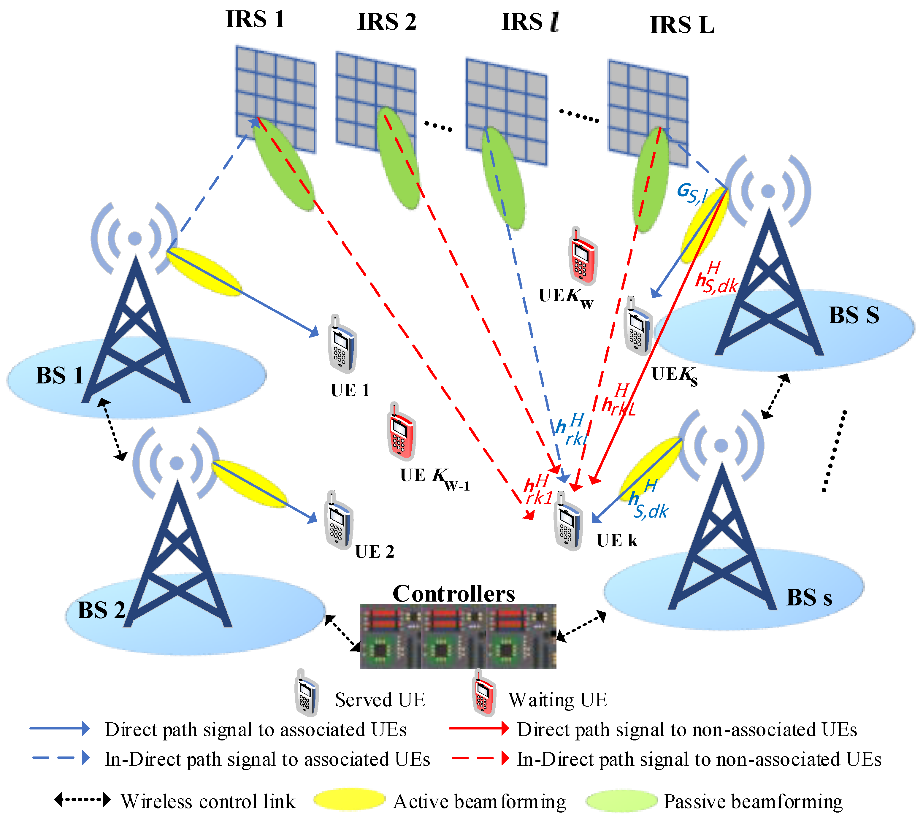
  • We develop a large-scale communication system with multi-BS assisted by multi-IRS to serve multi-UE. We formulate a comprehensive optimization problem aimed at maximizing the data rates of served UEs. The joint optimization encompasses BSs’ transmit powers, IRSs’ passive beamforming, and the design of BS–UE–IRS associations, all subject to the system and UEs’ QoS requirements.
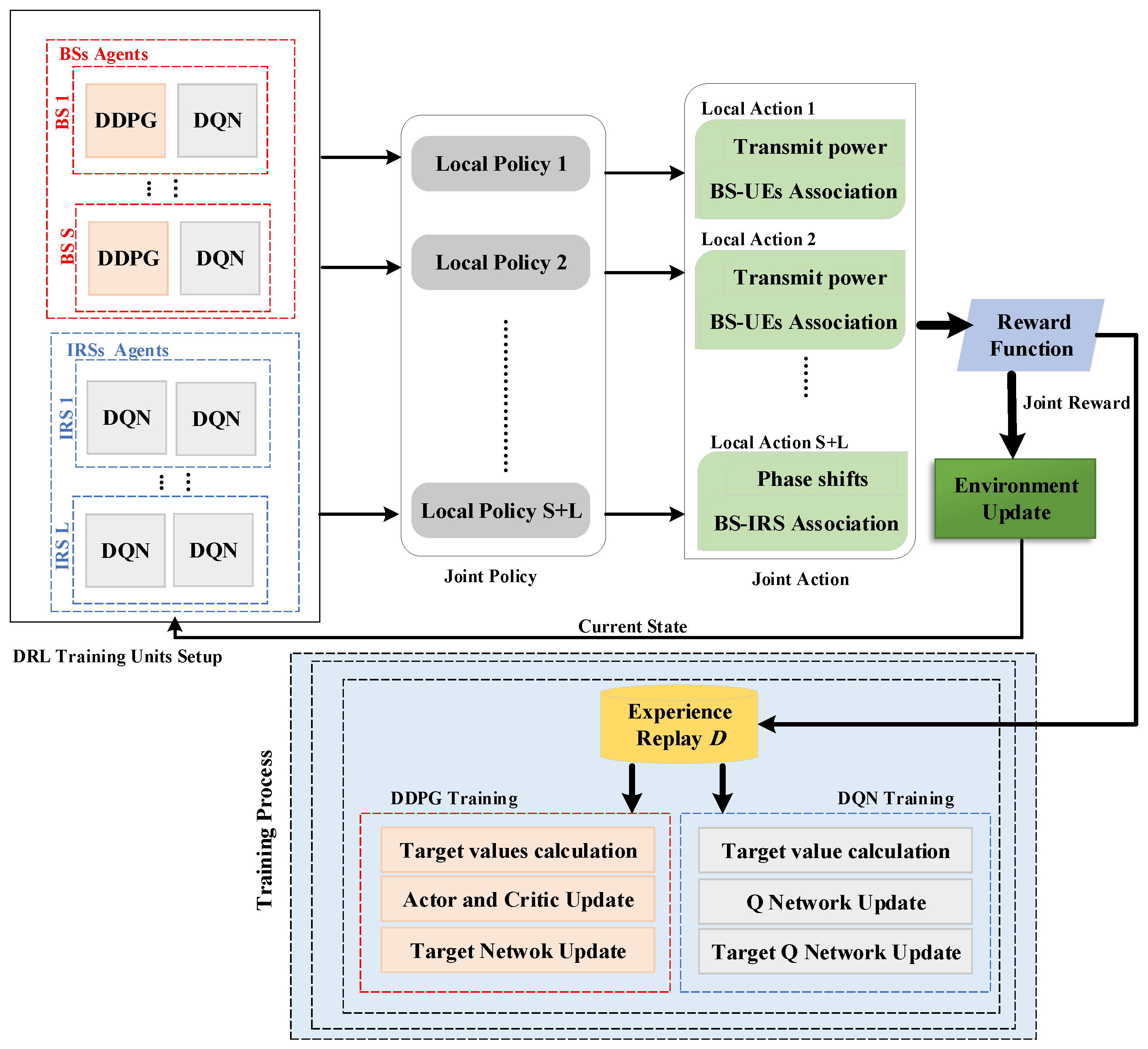
  • Addressing the inherent non-convexity of the original optimization problem, we propose a MADRL-based algorithm under continuous and discrete phases of the IRS scenarios. The optimization problem is modeled as an MAMDF, where the agents are designed by integrating DDPG and DQN algorithms to learn a joint policy. This approach enables the system to dynamically adapt to changing environmental conditions and maximize the long-term total system utility.
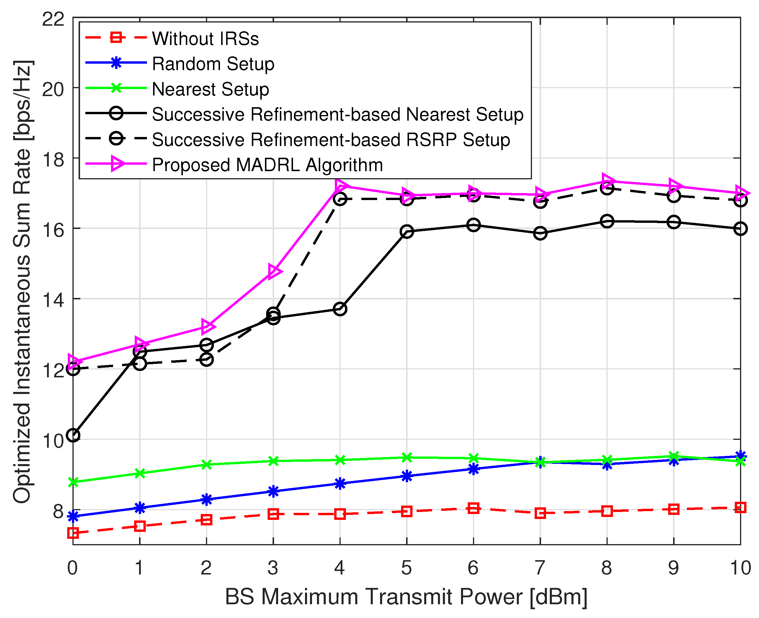
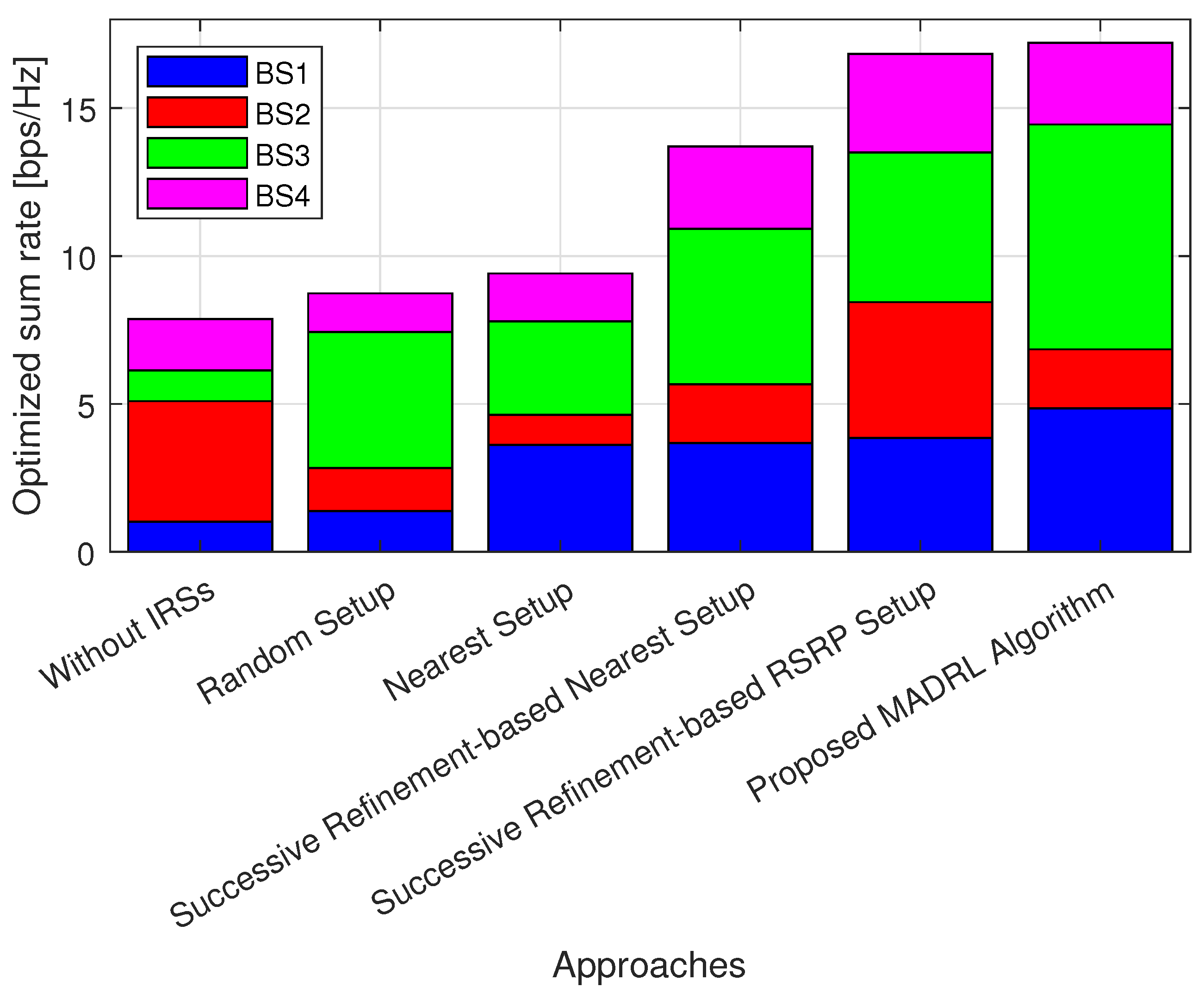
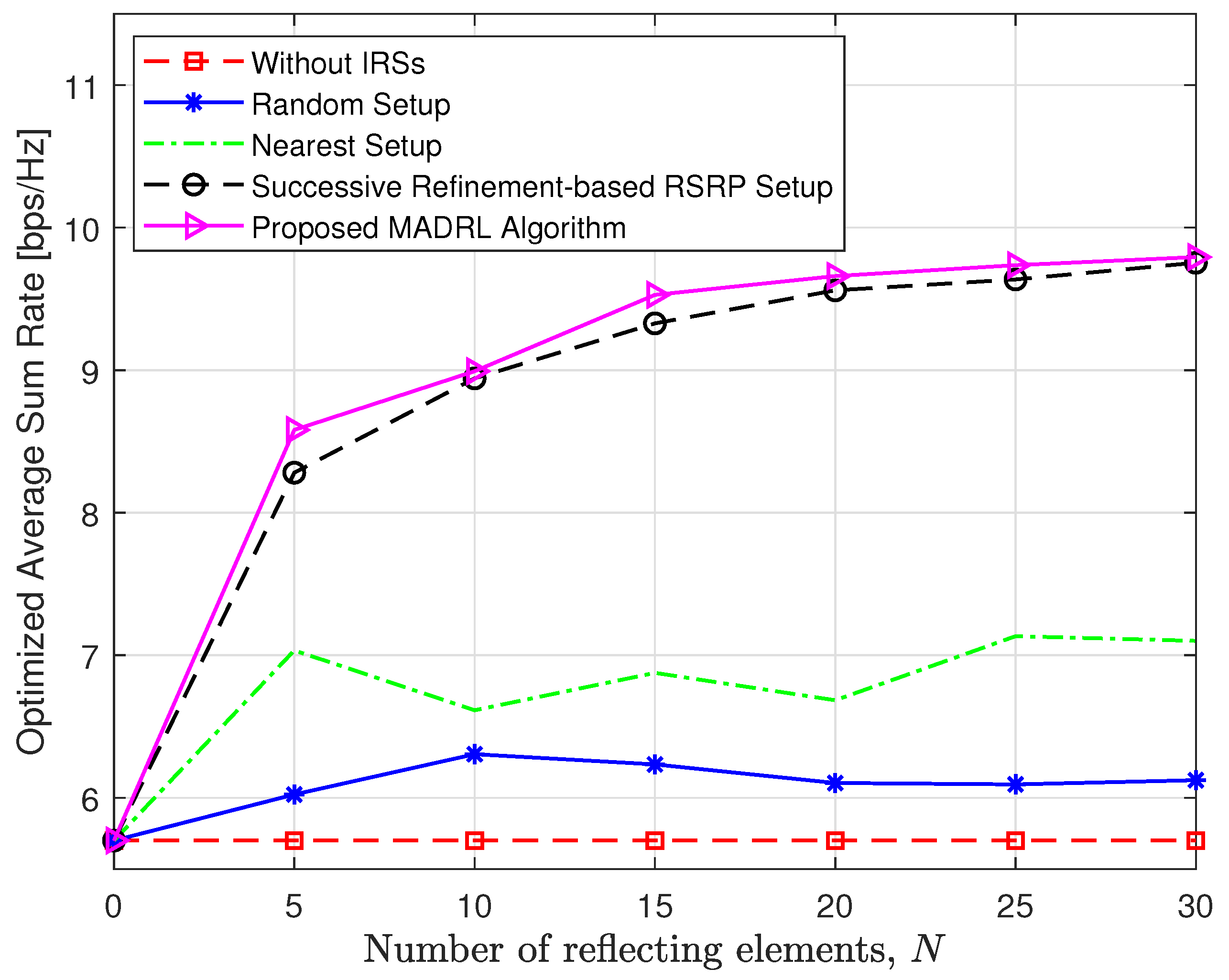
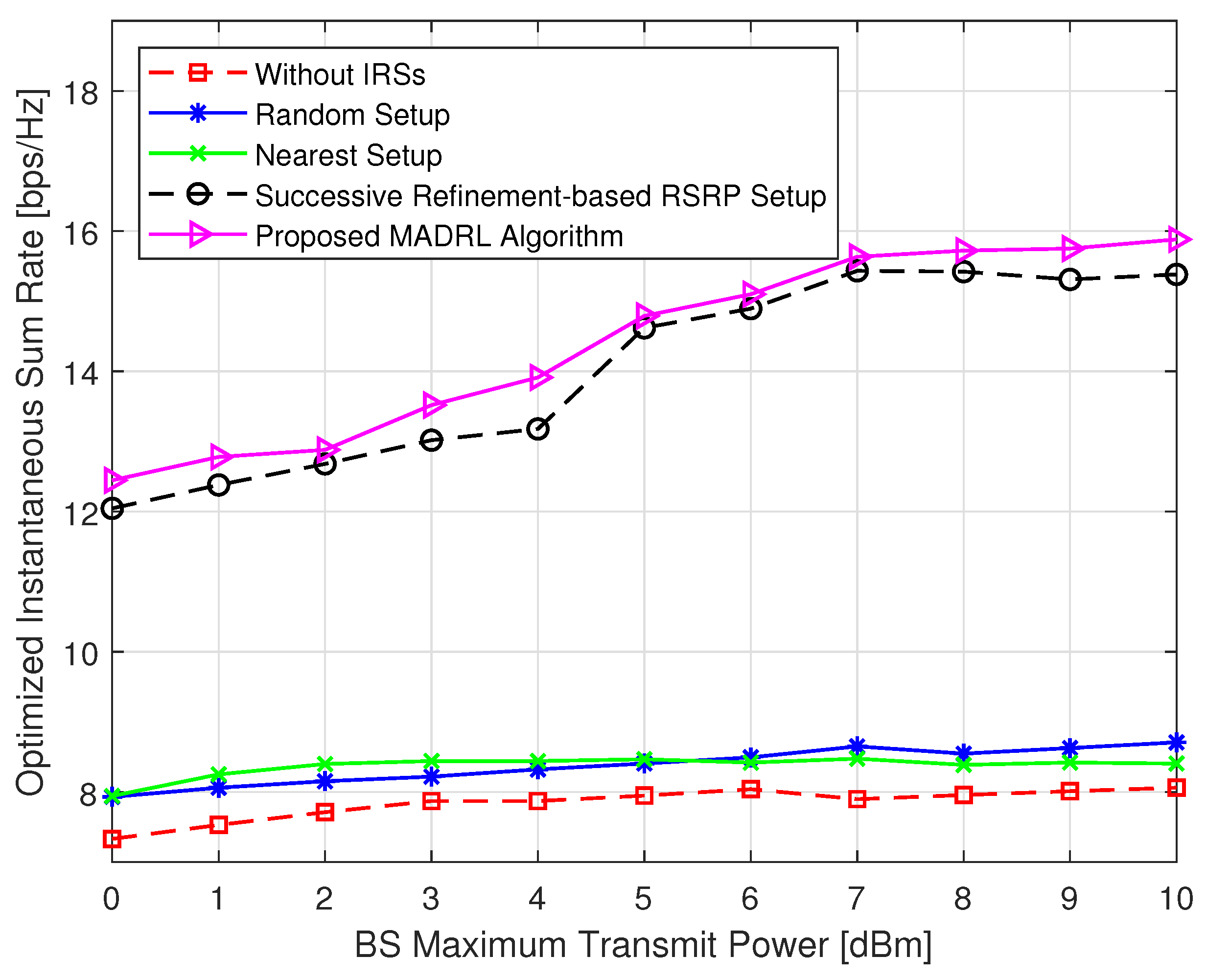
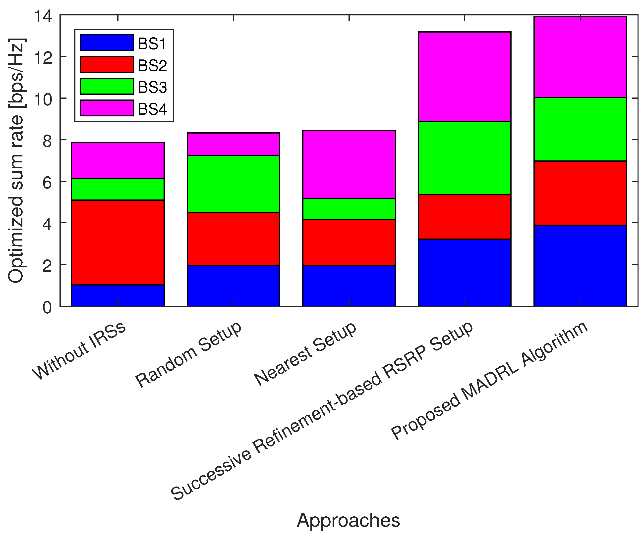
  • We analyze the convergence, computational complexity, and implementation efficiency of the proposed MADRL-based algorithm, integrated with the DRL algorithms. Our numerical results not only showcase the superior performance of our algorithm over benchmark schemes (e.g., the successive refinement-based approach), but also demonstrate its efficiency in terms of implementation runtime, thus validating its practical feasibility. Moreover, the achieved rate in the IRS-aided system exhibits substantial improvements as the number of reflecting elements increases, highlighting the scalability and effectiveness of the proposed approach.
The rest of this paper is structured as follows: Section 2 outlines the system model. Section 3 presents the formulated optimization problem. Section 4 details the proposed MADRL-based algorithm for continuous and discrete phases of the IRS configurations. Following that, Section 5 presents the simulation results. Finally, Section 6 provides a summary of the work.
Notation: Italicized letters represent scalars, while boldface is used for vectors and matrices. The . T and ( . ) H superscripts indicate transpose and Hermitian operations, respectively, while C signifies the complex domain. The notation CN μ , σ 2 denotes a circularly symmetric complex Gaussian (CSCG) distribution with mean μ and variance σ 2 . The notations . , . , . , and E [ . ] represent the Euclidean norm, absolute value, floor, and expectation, respectively. Moreover, Mod(.) represents the modulo operation; diag ( x ) denotes a diagonal matrix constructed with the elements of the vector x as its diagonal entries; log ( . ) denotes the logarithm function; f represents the gradient of f; and the order of complexity is denoted by O ( . ) .

2. System Model

As shown in Figure 1, we consider a downlink large-scale system assisted by multi-IRS to aid the communication between the multiple BSs and multiple UEs. Let the sets of multi-BS, multi-UE, and multi-IRS be denoted as S = { 1 , , S } , K = { 1 , , K } , and L = { 1 , , L } , respectively. At each time instance, the set of UEs can be divided into K s serving UEs and K w waiting UEs, with sets K s = { 1 , , K s } , and K w = { 1 , , K w } , respectively, where K s K w = K . Each BS is equipped with M transmit antennas, and each UE is equipped with a single antenna. Each IRS is a 2D surface composed of N = N H N V reflecting elements arranged in a rectangular grid. Here, N H represents the number of elements per row, and N V represents the number of elements per column. In addition, a wireless controller connects to the BS to configure the elements of the IRS [33]. Let the binary variables ρ k , s , k K , s S , represent the association indicator between the k-th UE and the s-th BS, where ρ k , s = 1 indicates that the k-th UE is associated with the s-th BS; otherwise, ρ k , s = 0 . It is assumed that each UE can be served from a maximum of one BS and, in turn, each BS is restricted to serving only one UE at any given time instant. The binary variables, λ l , s , l L , s S , denote the association indicator between the l-th IRS and the s-th BS, where λ l , s = 1 indicates that the l-IRS is associated with the s-th BS; otherwise, λ l , s = 0 . Furthermore, it is assumed that each IRS can be associated with only one BS at a given time instant. Accordingly, we can define the constraints of BS–UE–IRS associations at each node as follows:
s S ρ k , s 1 , k K ( UE association ) , k K ρ k , s 1 , s S ( BS association ) , s S λ l , s = 1 , l L ( IRS association ) .
We assume quasi-static, flat-fading channels. Specifically, the direct channel is denoted as h s , d k H C 1 × M , which represents the channel from the s-th BS to the k-th UE, while the indirect channels, G s , l C N × M and h r k l H C 1 × N , represent the channels from the s-th BS to the l-th IRS and from the l-th IRS to the k-th UE, respectively. As for the channel models, the BS–UE channels are modeled as Rayleigh fading, h s , d k H = PL s , k h ˜ s , d k H , where PL s , k is the s-th BS-k-th UE channel path loss, and h ˜ s , d k H follows CN ( 0 , 1 ) . The IRSs are positioned to maintain line-of-sight (LOS) connections between the BSs and the UEs. Consequently, the channels for BS–IRS and IRS–UE follow Rician fading, G s , l = PL s , l ( ε 1 + ε G ˜ s , l ( LOS ) + 1 1 + ε G ˜ s , l ( NLOS ) ) and h r k l H = PL k , l ( ε 1 + ε h ˜ r k l H ( LOS ) + 1 1 + ε h ˜ r k l H ( NLOS ) ) , respectively. Here, PL s , l and PL k , l are the path losses of the s-th BS to the l-th IRS channel and the l-th IRS to the k-th UE channel, respectively, and ε is the Rician factor. The NLOS components, G ˜ s , l NLOS and h ˜ r k l H ( NLOS ) , exhibit a distribution following CN ( 0 , 1 ) . The LOS elements are formulated as per [34], that is, G ˜ s , l LOS = a IRS ( ϑ s , l , ψ s , l ) a BS ( ϑ s , ψ s ) H and h ˜ r k l H ( LOS ) = a IRS ( ϑ l , k , ψ l , k ) H . Here, a IRS and a BS are the steering vectors for IRS and BS, respectively. The symbols ϑ and ψ represent the azimuth and elevation angles. For the l-th IRS steering vector, the n-th element can be calculated as [ a IRS ( ϑ l , k , ψ l , k ) ] n = e j 2 π d l λ c { i 1 ( n ) sin ( ϑ l , k ) cos ( ψ l , k ) + i 2 ( n ) sin ( ψ l , k ) } , where λ c denotes the carrier wavelength, d l represents the distance between adjacent elements of the l-th IRS, i 1 ( n ) = mod ( n 1 , N H ) , and i 2 ( n ) = ( n 1 ) / N H . Let the BSs, IRSs, and UEs coordinates be denoted as ( x s , y s , z s ) , ( x l , y l , z l ) , and ( x k , y k , z k ) . Accordingly, we set sin ψ l , k = ( z k z l ) / d k l and sin ( ϑ l , k ) cos ( ψ l , k ) = ( y k y l ) / d k l . Here, d k l represents the distance between the k-th UE and the l-th IRS. Also, a BS ( ϑ s , ψ s ) = [ 1 , , e j 2 π ( M 1 ) d s λ c cos ( ϑ 1 ) cos ( ψ 1 ) ] , where d s is the distance between adjacent antennas at the s-th BS. We set cos ( ϑ s ) cos ( ψ s ) = ( x l x s ) / d s l , where d s l represents the separating distance between the the s-th BS and the l-th IRS. Likewise, the steering vector a IRS ( ϑ s , l , ψ s , l ) can be computed, with sin ( ϑ s , l ) cos ( ψ s , l ) = ( y s y l ) / d s l , and sin ( ψ s , l ) = ( z s z l ) / d s l . Note that reciprocity between downlink and uplink channels is assumed.
At the transmitting side, each BS transmits its signal with a beamforming vector to serve its associated UE. Hence, the transmitted signal by the s-th BS takes the form of:
x s = p s w s s s ,
where p s is the transmit power, w s C M × 1 denotes the beamforming vector, and the transmit signal, denoted as s s , is characterized by random variables with a mean of zero and a variance of E s s 2 = 1 , which holds for all UEs. We assume each BS applies the maximum ratio transmission (MRT) precoding based on both direct and indirect channels with its served UE for active beamforming design, i.e.,
w s = H k H H k H ,
where H k = h s , d k H + l L h r k l H Θ l G s , l indicates the overall channel from the s-th BS to its served k-th UE; hence, E x s 2 = p s , i.e., p s 0 .  
At the reflecting side, the l-th IRS adjusts the received signals from all BSs and subsequently reflects them. In particular, each n-th element of the l-th IRS reflects the incident signal, x ^ s , n , multiplied by a complex factor of reflection. Therefore, the mathematically defined expression for the adjusted reflected signal at the l-th IRS by the n-th element, resulting from the incident signal from the s-th BS, is as follows:
y ^ s , l , n = β l , n e j θ l , n x ^ s , n , s , l , n ,
where β l , n 0 , 1 and θ l , n F l = [ 0 , 2 π ) represent the amplitude and angle for the n-th element of the l-th IRS, respectively, and F l denotes the set of phase-shift values at each element. Note that in practical implementation, it is considered that each n-th element n-th of the l-th IRS is limited to a finite set of discrete values. Therefore, for discrete phase shifts in the l-th IRS, the angle of the n-th element is determined as θ l , n F l = 0 , 2 π 2 b , , 2 π ( 2 b 1 ) 2 b , where b denotes the number of bits used to determine the number of phase shift levels at each element. As such, the l-th IRS maps from the s-th BS incident signal vector to a corresponding reflected signal vector using the reflection beamforming matrix Θ l , which is the main characteristic for each IRS. Therefore, the reflected signal at the l-th IRS due to the s-th BS incident signal is:
y ^ s , l = Θ l x s ^ , s , l ,
where x s ^ = [ x ^ s , 1 , , x ^ s , N ] T , and Θ l = diag ( β l , 1 e j θ l , 1 , , β l , N e j θ l , N ) C N × N and y ^ s , l = [ y ^ s , l , 1 , , y ^ s , l , N ] T . We further set β l , n = 1 , l , n in this system for maximizing the reflected signal by the IRSs [2,4].
At the receiving side, the k-th served UE K s receives its desired signal both from its associated BS via the direct path as well as the indirect paths from the reflections and the scattering of the associated and non-associated IRSs, respectively. Considering the substantial path loss, only the first signal reflected by the IRSs is taken into account, while the others are ignored. Hence, the desired signal received at the k-th UE from the s-th BS is calculated as follows:   
y k , s = h s , d k H p s w s s s + l L h r k l H Θ l G s , l p s w s s s = h s , d k H p s w s s s + l L λ l , s h r k l H Θ l G s , l p s w s s s Associated IRSs + l L ( 1 λ l , s ) h r k l H Θ l G s , l p s w s s s Non - associated IRSs , k K s .
Meanwhile, the k-th UE is affected by co-channel interference from the S 1 non-associated BSs that serve the other K 1 UEs through direct and indirect links via all deployed IRSs. Thus, the total interference signal affecting the k-th UE is expressed as:
I ¨ k = i S , i s h i , d k H p i w i s i + i S , i s l L h r k l H Θ l G i , l p i w i s i Inter-cell interference (co-channel interference)   I k + n k Noise , k K s ,
where n k is modeled as CN 0 , σ k 2 , k K . Therefore, the signal-to-interference-plus-noise ratio (SINR) observed at the k-th UE, associated with the s-th BS, is formulated as:
SIN R k , s = y k , s 2 I k 2 + σ k 2 , k K s .
Then, the achievable rate of the k-th UE, expressed in bps/Hz, is determined as:
R k , s = s S ρ k , s log 2 ( 1 + SINR k , s ) , k K s .
Accordingly, we define the system utility as the sum rate of all served UEs by:
R sum = k K s R k , s = k K s S ρ k , s log 2 ( 1 + SIN R k , s ) .

3. Formulation of the Optimization Problem

The target of this work is the maximization of the system utility by maximizing the sum rate of the served UEs while still guaranteeing their rate constraints by jointly optimizing BS–UE associations ρ k , s , BS–IRS associations λ l , s , IRSs beamforming matrices { Θ l } l = 1 L , and BSs power control P . Therefore, we formulate the optimization problem as:
( P 1 ) : max ρ k , s , λ l , s , { Θ l } l = 1 L , P R sum
s . t . R k , s R min , k K s , s S ,
s S ρ k , s 1 , k K ,
k K ρ k , s 1 , s S ,
s S λ l , s = 1 , l L ,
θ l , n F l , l , n ,
0 p s p max , s S ,
ρ k , s { 0 , 1 } , λ l , s { 0 , 1 } , l L , s S , k K .
Note that (P1) is a challenging mixed-integer nonlinear programming (MINLP) problem due to its non-convex nature and the coupling between the objective function and constraints. The inclusion of binary variables ρ k , s and λ l , s introduces combinatorial aspects and NP-hardness. Generally, to optimally solve this problem, a relaxation conversion can be applied to transform the original non-convex problem into a convex formulation. To be specific, applying convex relaxation to the objective involves using the concave envelope, e.g., the exponential function, to approximate the logarithmic function. For the constraints, the problem has two types of non-convex constraints: the discrete constraints of passive beamforming and the binary constraints of association matrices. The discrete constraints can be relaxed by applying the semidefinite programming (SDP) technique by allowing continuous phase shifts. Meanwhile, the binary constraints can be replaced with continuous variables constrained between 0 and 1. Then, use a penalty function to enforce the binary nature. A convex optimization solver capable of handling mixed-integer and continuous variables, such as CVX [35], can solve the resulting convex-relaxed optimization problem. Based on our large-scale system, solving large-scale mixed-integer convex problems can be computationally demanding, especially with SDP relaxations, which can lead to computationally expensive solutions. However, with the discrete phase shift configuration and fixing BSs’ power, or when relaxed to discrete counterparts, the optimization can be solved optimally by enumerating all feasible possible combinations. Nevertheless, this approach incurs high complexity, which becomes prohibitive with a large number of BSs, UEs, and IRSs. Note that in case of the continuous configurations to the IRSs and considering constraint (11d), the phases can be determined by the instantaneous CSI, as the direct and indirect channels are aligned in phase to serve the associated UE [4]. Thus, the n-th phase shift of the l-th IRS is calculated as:
θ l , n = h r k l , n ( g s , l , n H h s , d k ) ,
where h r k l , n is the n-th element of h r k l H and g s , l , n H is the n-th row vector in G s , l . Additionally, some strategies and algorithms have been applied to find sub-optimal solutions to association matrices with given other optimization variables. Specifically, the maximum reference signal received power (RSRP) association-based method is commonly used for designing BS–UE associations [36]. Let ρ s = [ ρ 1 , s , ρ 2 , s , , ρ k , s ] represent the solution for BS–UE associations and the received powers from the s-th BS to UEs are denoted as P s r = [ P 1 , s r , P 1 , s r , , P k , s r ] , where P k , s r = y k , s 2 . Accordingly, each BS s -th BS serves k -th UE, with k = argmin i P i , s r . This rule needs a prior design for phase shifts of the IRS elements to determine the total received signals at the UEs from the indirect paths. Furthermore, sub-optimal solutions for BS–IRS associations can be obtained with convergent results using the successive refinement algorithm [14]. This iterative algorithm updates the associated BS for each deployed IRS successively, while keeping the associations of all other IRSs fixed until no further improvement in the defined performance can be achieved. Specifically, consider the BS-IRS association solution as λ l = [ λ l , 1 , λ l , 2 , , λ l , S ] , l L . For a given design of BS-IRS association, represented by { λ l } for all L IRSs, let R sum ( λ l ) denote the corresponding maximum sum rate. During algorithm iteration, each l -th IRS optimizes λ l successively, while the associated BSs for all other IRSs, denoted as { λ l } l l , are fixed to maximize R sum ( λ l ; { λ l } l l ) . Enumerating the S BSs for the l -th IRS efficiently obtains the optimal solution to l . Subsequently, the associated BS for the l -th IRS is updated, and this process continues for the next IRS. Thus, this algorithm is a timely strategy since it needs to solve many iterations until there is no further improvement in its performance.
The challenges within our large-scale system stem from intricate interactions and dependencies among diverse entities, including BSs, UEs, and IRSs. These entities are intricately linked through associations, beamforming, and power control decisions, introducing complexity to the optimization of resources. Associations dictate which UEs are served by specific BSs and IRSs, while the beamforming matrices of IRSs impact signal propagation characteristics. The mobility of UEs and the non-convex nature of the optimization problem add to the complexity. Facilitating enhanced coordination and adaptability becomes crucial for efficient resource utilization and interference minimization amid dynamic network conditions. Enhanced coordination ensures harmony among network entities, while adaptability permits dynamic adjustments to configurations and strategies. To tackle these challenges, we propose the MADRL approach. In MADRL, each agent, representing a network entity, autonomously learns and refines its decision-making policy through collaborative learning. This approach not only ensures fair resource allocation, minimum rate requirements, and efficient power usage, but also enhances the overall adaptability and coordination of the network in dynamic conditions.

4. Proposed MADRL-Based Algorithm

In this section, we present the proposed MADRL-based algorithm. We begin by reformulating the optimization problem in the form of an MMDP. Subsequently, we detail the proposed algorithm, considering two configurations of the IRS. Finally, an analysis of the algorithm’s convergence and complexity is provided.

4.1. MAMDP Formulation of the Optimization Problem

To apply MADRL, the initial step involves transforming the optimization problem into an MAMDP format. The MAMDP typically comprises five essential elements for each agent: agent i, state s t i , action a t i , reward function r t i , and policy π t i [37].
Given our studied system and formulated optimization problem, the behavior of all BSs and IRSs is modeled as a MADRL MMDP, which involves a set of agents (i.e., BSs and IRSs): G = { S L } . Thus, we have a total of states sets { S j } j = 1 S + L , actions { A j } j = 1 S + L , and rewards { R j } j = 1 S + L . Under the MAMDRL, at each time step t, each agent receives an immediate observation or state s t i S i from the environment, where S i represents the potential set of states for agent i. In response to this state, each agent chooses an action a t i A i , where A i denotes the set of possible actions for agent i. Subsequently, the environment updates the states to the next states s t + 1 i and supplies a performance metric reward r t i for that state–action pair ( s t i , a t i ) . The mapping from states to actions, governed by each agent’s local policy π t i ( s t i , a t i ) , signifies the probability of selecting action a t i for the current state s t i . Over time, each agent strives to learn an optimal policy by maximizing cumulative rewards in the collaborative multi-agent environment. All the agents operate independently in a shared environment and then form joint action a t = { a t 1 , a t 2 , , a t S + L } A , where A = { A 1 , A 2 , , A S + L } . The subsequent state s t + 1 is updated from the current s t = { s t 1 , s t 2 , , s t S + L } providing the joint rewards r t = { r t 1 , r t 2 , , r t S + L } R to the joint state–action pairs. Accordingly, the joint optimal policy π t ( s t , a t ) = { π t 1 ( s t 1 , a t 1 ) , π t 2 ( s t 2 , a t 2 ) , , π t S + L ( s t S + L , a t S + L ) } is formed, which can maximize the long-term rewards received. The states, actions, rewards, and policies of our proposed MADRL-based approaches are described below.
  • States: For each BS agent j S , we define its state as the current active beamforming at time step t, ( w j ) t , the previous transmit power at time step t 1 , ( p j ) t 1 , the previous BS–UE associations vector at time step t 1 , ( { ρ k , j } k = 1 K ) t 1 , the previous BS-IRSs associations vector at time step t 1 , ( { λ l , j } l = 1 L ) t 1 , and the current position to the served UE, ( { ( x k , y k , z k ) } ) t , k K s , which is mathematically given by:
    s t j = ( w j ) t , ( p j ) t 1 , ( { ρ k , j } k = 1 K ) t 1 , ( { λ l , j } l = 1 L ) t 1 , ( { ( x k , y k , z k ) } ) t S ,
    whose dimension is 2 M + K + L + 4 . The term ( w j ) t , determined by the CSI, serves as a surrogate for the CSI in s t j at time t to capture variations in wireless channel conditions. Note that directly integrating the channel estimates among all system nodes into the local observation may not be feasible due to the impracticality of handling high-dimensional feedback, while for each IRS agent l L , we define its state as the previous passive beamforming vector at time step t 1 , ( θ l ) t 1 , which is defined as:
    s t l = { ( θ l ) t 1 } S ,
    whose dimension is 2 N .
  • Actions: For each BS agent j S , its action includes the transmit power, ( p j ) t , BS–UE association vector, ( { ρ k , j } k = 1 K ) t , and BS-IRSs associations vector, ( { λ l , j } l = 1 L ) t . However, in order to handle constraint (11e) and reduce the action space of the BS–IRS associations from L · S to L, we shift the BS-IRSs associations as a subfunction to IRS agents, where each IRS has to choose one BS. Moreover, in order to reduce the infeasible BS–UE association actions and handle constraints (11c) and (11d) during training, a centralized DRL element for all BS–UE associations is trained at one BS, and then a copy is delivered to all BSs. Consequently, the action of each BS agent j is denoted by:
    a t j = { ( p j ) t , ( ρ k , j ) t } A ,
    where ( ρ k , j ) t is the index of the served k-th UE by the s-th BS. Correspondingly, the dimension is simply 2, and the action space of BS–UE associations equals K, while for each IRS agent l L , we define its action as the current passive beamforming, ( θ l ) t , and BS-IRS association index element, ( λ l , j ) t , where λ l , j is the index of the chosen j-th BS for l-th IRS. For example, if at time step t, the agent IRS l chose to associate with the fourth BS, then ( λ l , 4 ) t = 1 in the BS–IRS associations matrix. The action of each IRS agent l is denoted by:
    a t l = { ( θ l ) t , ( λ l , j ) t } A .
    which outputs a dimension of 2 N + 1 and an action space of BSs-IRS associations of S.
  • Rewards: As the objective function of the optimization problem is to maximize the sum rate of served UEs, establishing a connection between the reward and the objective function drives the realization of the MMDP goal to augment long-term rewards. Noting that each agent with a separate reward may behave selfishly, therefore hindering the global optimal solution. Thus, we assume all agents have the same reward after the joint action is performed. The environment sets the instant reward for all cooperative agents in this framework as the total sum rate achieved. Note that all the constraints in (P1) are handled above, except the constraint (11b), which considers the minimum QoS requirements constraints. If the resulting joint action fails to satisfy the minimum data rates of the UEs, agents are penalized to encourage them to modify inappropriate actions. The reward function includes a penalty value, which is represented by the difference between the minimum achieved rate and the specified constraint rate. Thus, the agents will receive a negative penalty if the minimum QoS is not satisfied for the UEs. Otherwise, all agents will receive positive rewards represented by the total utility achieved. Here, we set such a penalty value instead of zero to limit the sparsity of the rewards and reflect how far the agents are from achieving the minimum QoS. Therefore, each agent i G can receive an instant reward, determined as follows:
    r t i = ( R sum ) t , if ( R k , s ) t R min , k K s , s S , | ( R k min ) t R min | , if ( R k , s ) t < R min , k K s , s S ,
    where R k min represents the minimum achieved data rate of all the served UEs at the t-th time step.
  • Policies: In the proposed MADRL framework, effective collaboration hinges on creating an optimal joint policy, denoted as π t ( s t , a t ) . This joint policy plays a pivotal role in guiding collective decision-making among agents, directing them to choose actions that enhance cumulative rewards in the dynamic multi-agent environment. The process of learning and contributing to this joint policy is iterative and adaptive for each agent. In response to ever-changing environmental states, agents continually adjust their local policies by evaluating the outcomes of their actions based on observed states. Reinforcement signals aid this learning process, guiding agents toward actions that maximize system utility over the long term through reward-based feedback. Further sections will provide a closer look at how agents refine their local policies, contributing to the overall success of the collaborative MADRL framework.

4.2. The Implementation of the Proposed MADRL-Based Algorithm

In this subsection, the proposed MADRL-based algorithm frameworks are described in detail to solve the optimization problem under continuous and discrete phases of the IRSs. These proposed algorithms mainly consist of two phases, namely training and implementation. Each phase will be detailed below.

4.2.1. MADRL-Based Algorithm under Continuous Phases Case

Note that conventional one-agent-DRL-based approaches can be applied to solve the problem (P1) by exploring all possible actions. However, in this work, the problem has huge state and action spaces with both continuous and discrete optimization variables, posing challenges for applying a one-agent-based approach. Accordingly, we propose a cooperative MADRL-based framework to handle the challenges and solve the problem efficiently, where the multi-agent-based approach can work together to reduce the state and action spaces. Since the joint action includes both discrete and continuous actions, we apply different DRL algorithms to train the agents.
As shown in Figure 2, for each BS agent, we apply two DRL units: deep deterministic policy gradient (DDPG) to optimize transmit power allocation, ( p j ) t , j S , and deep Q-network (DQN) to optimize BS–UE associations vector, ( { ρ k , j } k = 1 K ) t . For each IRS agent, we apply two DRL units: DDPG for continuous phases, i.e., ( θ l ) t and DQN for BSs-IRS associations vector, i.e., ( { λ l , j } l = 1 L ) t . Note that, according to our system design, we have a closed form (12) to obtain continuous phases by knowing the associations’ designs; thus, we do not need DDPG units for the phases at the IRSs in the continuous case. In addition, we implement a centralized DDPG unit that copies the local action to each BS for controlling their transmit powers. Additionally, all the DRL algorithms are connected to replay memory to store all trained experiences, where a central control is employed to control the local and joint experiences.
The DQN algorithm integrates deep neural networks (DNNs) with Q-learning, where the DNNs are used to approximate the Q-function, replacing the tabular representation for the Q-value function. DQN consists of two networks, i.e., one is the main neural network called Q network with parameters θ q , which estimates the Q-value for the current state and action pair. The other is a target Q network with parameters θ q . Note that θ q and θ q have identical structures, but θ q is used to estimate the Q-values of the next step state–action pair. Furthermore, the DQN algorithm stores all acquired experiences in the integrated replay memory. Figure 3a illustrates the architecture of the DQN algorithm. Meanwhile, the DDPG algorithm follows the DPG theorem, which learns a Q-function and a policy simultaneously. It can deal with continuous action spaces, addressing the restriction of the DQN network to discrete action spaces only. As illustrated in Figure 3b, DDPG consists of four networks, i.e., the actor-network with parameters θ μ , the target actor-network with θ μ , the critic-network with parameters θ q , and the target critic-network with θ q . Specifically, the DDPG algorithm trains the actor network to select the best actions given the current state, while the performance critic network estimates Q-value performance. Similar to DQN, the target networks mirror the structure of the training networks but have distinct parameters, and they utilize experience replay memory.
Given the structure of the DRL algorithms outlined above, we employ the proposed algorithm to solve (P1), as outlined in Algorithm 1. In the beginning, the integrated networks for all DDPG and DQN units are initialized, and all training hyper-parameters are set. Assuming the agents’ interactions within the environment are segmented into I episodes, each comprising a finite number of T steps. Then, at the start of every training episode, the algorithm resets the environment with different locations for the UEs and their corresponding channel gains. Subsequently, all channels linking network nodes are computed. We apply Additionally, random initialization is applied to the transmit powers, beamforming vectors, and association matrices. Accordingly, the state s t is defined and provided as input stimulation. The agents then provide feedback on the decisions of local actions related to the integrated DRL units at each agent to form the joint action. Then, the BSs’ transmit powers, BSs’ active beamforming, IRSs’ passive beamforming, and BS–IRS–UE association matrices are formulated. Thereby, the current joint reward is computed, and the subsequent state s t + 1 is defined. This information is stored as the joint experience { s t , a t , r t , s t + 1 } to create the integrated buffer. This algorithm requires a minimum of N B experiences to initiate network updates and learning. Consequently, the preceding steps are reiterated N B times to establish the initial mini-batch, but this occurs exclusively in the first episode. Following the creation of N B experiences, the algorithm proceeds to the training phase. Note that the flow chart of Algorithm 1 is figured in Figure 4 to provide a visual representation of the algorithmic steps and facilitate better understanding.
At each time step t, the algorithm extracts local states, actions, and rewards from the chosen N B samples. Specifically, during the learning process, the action value function of each agent j is updated according to the Bellman equation as follows:   
Q j ( s t j , a t j ) Q j ( s t j , a t j ) + α r t j + γ max a j Q j ( s t + 1 j , a j ) Q j ( s t j , a t j ) ,
where α denotes the learning rate. Therefore, each agent j obtains the optimal value function by solving:
Q * j ( s t j , a t j ) = E s t + 1 j r t j + γ max a j Q * j ( s t + 1 j , a t j ) | s t j , a t j ,
where ( s t + 1 j , a t + 1 j ) represents the next state–action pair for agent j.
With the DQN algorithm structure, each agent j with a current state s t j selects its action a t j using ϵ -greedy exploration. The agent either chooses a random action with a probability of ϵ or selects an action for which the value function Q is greatest with a probability of 1 ϵ .
a t j = random action , with probability ϵ , argmax a t j A j Q ( s t j , a t j ) , with probability 1 ϵ .
Since the association designs and IRS reflection phases are shared by the system nodes, fully distributed operation for the agents without environment state sharing may be infeasible for a large-sized network. In our cooperative multi-agent framework, we adopt independent learning with state and reward sharing, where all agents form a joint action and calculate the reward in (17). With this joint response, a new state s t + 1 is formed, and a new experience { s t , a t , r t , s t + 1 } is added to the reply. A random sample of size N B is chosen from the replay to update the weights of the Q-network. Consequently, the target value function Q is given by:
y t j = r t j , if s t + 1 j is terminal state , r t j + γ max a t + 1 j A j Q ( s t + 1 j , a t + 1 j ; θ q ) , otherwise .
By using gradient descent, the Q network of agent j can be trained by minimizing the following DQN loss function, expressed as:
L ( θ q ) = ( y t j Q ( s t j , a t j ; θ q ) ) 2 .
Next, a smoothing update is applied to the target critic parameters, gradually adjusting them to track the changes in the critic network. This process helps stabilize the learning and prevent rapid fluctuations in the target values, as follows:
θ q τ DQN θ q + ( 1 τ DQN ) θ q ,
where τ DQN 1 represents the target smooth factor for the DQN algorithm. Subsequently, adjust the probability threshold ϵ for selecting a random action according to the decay rate α decay . At the end of each training step, if ϵ exceeds the minimum value ϵ min , it is adjusted as follows:
ϵ = ϵ ( 1 α decay ) .
Note that ϵ is maintained from the end of one episode to the beginning of the next one, resulting in a gradual, uniform decrease over multiple episodes until it reaches ϵ min .
Algorithm 1 The proposed MADRL-based algorithm.
1:
Initialize the power allocation DDPG units for all the BSs agents, including actor-network μ ( s ; θ μ ) , target actor network μ ( s ; θ μ ) , critic network Q ( s , a ; θ q 1 ) , target critic network Q ( s , a ; θ q 1 ) with parameters θ μ = θ μ and θ q 1 = θ q 1 .
2:
Initialize the BS–UE associations DQN units, including Q-network Q ( s , a ; θ q 2 ) , target Q-network Q ( s , a ; θ q 2 ) with parameters θ q 2 = θ q 2 .
3:
Initialize the passive beamforming DQN units for all the IRS agents, including Q-network Q ( s , a ; θ q 3 ) , target Q-network Q ( s , a ; θ q 3 ) with parameters θ q 3 = θ q 3 .
4:
Initialize the BS–IRS associations DQN units, including Q-network Q ( s , a ; θ q 4 ) , target Q-network Q ( s , a ; θ q 4 ) with parameters θ q 4 = θ q 4 .
5:
Initialize the learning rates α DQN and α DDPG , discount factor γ , target smooth factors τ DQN and τ DDPG mini-batch size N B and an empty experience replay D.
6:
for episode i = 1 , 2 , , I  do
7:
     Reset the environment and acquire ( x k , y k , z k ) , { h s , d k H } , { G s , l } , and { H r l } , s , l , k .
8:
     Initialize { p s } s = 1 S , { w s } s = 1 S , { Θ l } l = 1 L , { ρ k , s } and { λ l , s } , s , l , k .
9:
     Form initial state s 1 to all agents.
10:
   for step t = 1 , 2 , T  do
11:
     for agent j = 1 , 2 , , S + L  do
12:
        if  j S  then
13:
          Power allocation DDPG unit selects transmit power, i.e., ( p j ) t .
14:
          BS–UE association DQN unit selects ( ρ k , j ) t .
15:
          Form the action a t j of the BS j as (15).
16:
        end if
17:
        if  j L  then
18:
          Passive beamforming DQN unit selects ( θ l ) t .
19:
          BSs-IRS association DQN units select ( λ l , j ) t .
20:
          Form the action a t l of the IRS l as (16).
21:
        end if
22:
     end for
23:
     Form the joint action a t by all agents.
24:
     Form the BSs transmit powers ( { p s } s = 1 S ) t , the BSs active beamforming ( { w s } s = 1 S ) t , IRSs passive beamforming ( { Θ l } l = 1 L ) t and BS–IRS–UE associated matrices, i.e., ρ t , λ t .
25:
     Calculate the current joint reward r t using (17).
26:
     Form the next joint state s t + 1 for all agents.
27:
     Fill the buffer D by the experience { s t , a t , r t , s t + 1 } .
28:
     for agent j = 1 , 2 , , S + L  do
29:
        if update then
30:
          Select from the buffer a N B experiences { s i , a i , r i , s i + 1 } .
31:
          if  j S  then
32:
             Calculate the target values of the DDPG units according to (26).
33:
             Calculate the target values of the DQN units according to (21).
34:
             Update every U steps: θ μ according to (28), θ q 1 according to (27), θ μ according to (29), and θ q 1 according to (30).
35:
             Update θ q 2 according to (22), update θ q 2 according to (23).
36:
          end if
37:
          if  j L  then
38:
             Set the value function target of DQN units as (21).
39:
             Update θ q 3 according to (22), update θ q 3 according to (23).
40:
             Update θ q 4 according to (22), update θ q 4 according to (23).
41:
          end if
42:
        end if
43:
     end for
44:
     Assign the updated state as s t + 1 .
45:
   end for
46:
end for
The DDPG algorithm is employed for optimizing the transmit power of the BSs. In contrast to DQN, which employs an ϵ -greedy strategy, DDPG applies the DPG theorem to update the network parameters, estimating the current action from the current state. The action is evaluated using the deterministic policy of the actor network. To ensure effective exploration in the continuous action space during the DDPG training process, an exploration policy is formed by incorporating a defined noise into the DDPG action, as follows:
a t j = μ ( s t j ; θ μ ) + N t ,
where N t is the deployed noise model. Accordingly, the target value function for each agent j is calculated as follows:
y t j = r t j , if s t + 1 j is a terminal state , r t j + γ Q ( s t + 1 j , μ ( s t + 1 j ; θ μ ) ; θ q ) , otherwise .
During training, the algorithm updates the critic network through the minimization of the critic loss function based on the selected mini-batch samples, as follows:
L ( θ q ) = 1 N B t = 1 N B ( y t j Q ( s t j , a t j ; θ q ) ) 2 .
Following these, a policy gradient function is applied to update the actor network, involving the calculation of the derivative of the policy’s performance J with respect to θ μ , as computed below:
θ μ J = 1 N B t = 1 N B a j Q ( s t j , μ ( s t j ; θ μ ) ; θ q ) G a t | θ μ μ ( s t j ; θ μ ) G μ t ,
where G μ t and G a t denote the gradient of the actor output and the critic output concerning the actor parameters and the actor action, respectively. Next, a smoothing mechanism is adopted to update the target networks, expressed as follows:
θ μ τ DDPG θ μ + ( 1 τ DDPG ) θ μ ,
θ q τ DDPG θ q + ( 1 τ DDPG ) θ q ,
where τ DDPG 1 is the smooth factor for the target networks in the DDPG algorithm.

4.2.2. MADRL-Based Algorithm under Discrete Phases Case

Due to the practical implementation and hardware constraints, the n-th element of the l-th IRS generally takes a finite set of discrete values. Considering the discrete case of IRS phase shifts, we propose a cooperative MADRL-based framework under the discrete case in this subsection. The BS agents are similar to the case with continuous cases, where each BS agent j S , adopts a DDPG unit for power allocation, ( p j ) t , and a DQN unit for BS–UE associations, ( { ρ k , j } k = 1 K ) t . However, for the IRS agents, each IRS agent l L , adopts two DQN units, i.e., one to handle the discrete phase shift actions, i.e., ( θ l ) t , and the other for the BSs-IRS associations vector, i.e., ( { λ l , j } l = 1 L ) t , as shown in Figure 2.
During the implementation stage, the cooperative agents observe the environmental state and make decisions regarding the powers of the BSs, phases of the IRSs, and the configuration of associations based on the trained models. After that, they observe the updated state and make another decision. In this setting, we assume that the locations of the UEs are accessible to the BSs agents and then shared with IRSs agents; for example, predicting the location information involves processing the signals and channels during the uplink communication, including path loss coefficients, the angle of arrival (AoA), the angle of departure (AoD), and the time of arrival (ToA) [38]. The proposed MADRL-based algorithm integrates the contents of Section 4.2.1 and Section 4.2.2, and is summarized in Algorithm 1.

4.3. Analysis of the Proposed MADRL-Based Algorithm

In this subsection, we analyze the convergence and computational complexity of the proposed cooperative MADRL-based algorithm under continuous and discrete phases. Then, the implementation complexity is compared to benchmark schemes.

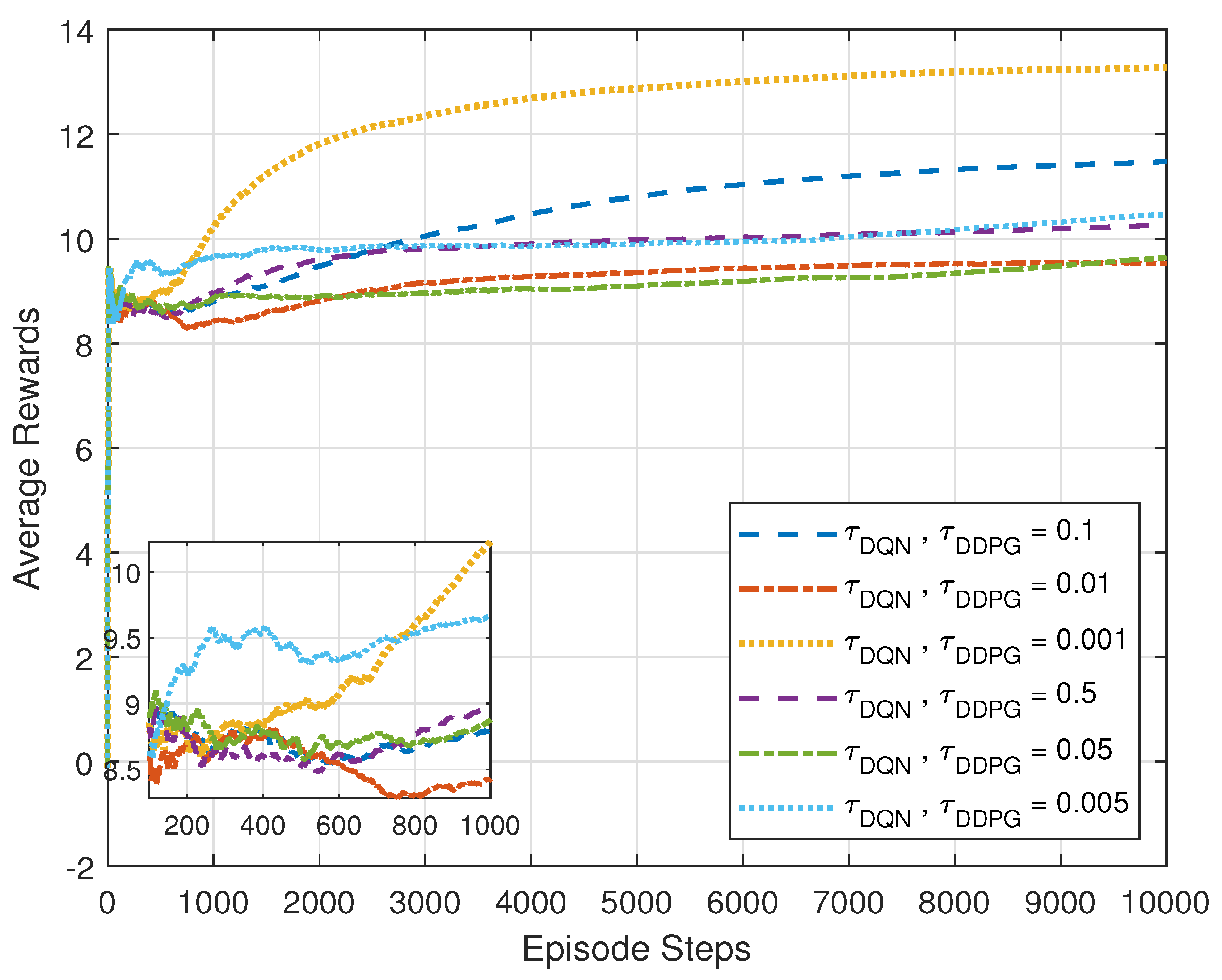
4.3.1. Convergence Analysis

The proposed cooperative MADRL-based algorithm integrates DQN and DDPG algorithms, which learn policies independently. Therefore, the convergence of the proposed algorithm relies on the convergence of the DDPG and DQN algorithms. Initially, we analyze the convergence of traditional Q-learning-based algorithms, as the DQN and DDPG algorithms are considered evolutionary extensions of Q-learning algorithms. According to [39], the Q-learning-based algorithm converges to the optimal Q-function when the learning rate guarantees 0 α t 1 , t α t = , and t α t 2 < . Moreover, consider I m as the m-dimensional unit hyper-cube [ 0 , 1 ] m , and φ ( t ) is a continuous function that is bounded, non-constant, and monotonically increasing. Additionally, C ( I m ) denotes the space of continuous functions on I m . For any provided function f C ( I m ) and ϵ > 0 , there exists a F ( x ) = i = 1 N v i φ ( w i T x + b i ) with real vector w i R m , ( i = 1 , , N ) , real constants v i , b i R , and integer N to obtain an approximation of the function f s realization. Note that f is independent of φ and guarantees | F ( x ) f ( x ) | < ϵ , x I m . In essence, functions represented by the form F ( x ) are densely distributed within C ( I m ) . Following the Stone–Weierstrass theorem [40], a large neural network and the proper choice of initial conditions can be used to get close to any non-linear continuous function. Thus, it can be concluded that the DQN algorithms converge to optimal solutions by a large-size neural network and appropriately tuned free parameters and initial parameters. For the DDPG algorithm, as it applies a deterministic policy gradient theory, it shows convergence to sub-optimal solutions [41]. In summary, the proposed cooperative MADRL-based algorithm is guaranteed to converge under both continuous and discrete phases.

4.3.2. Computational Complexity Analysis

The computational complexity of the proposed algorithm can be split into two primary parts: forward propagation and backpropagation for action selection and training models [31], respectively.
  • Action selection complexity: Let | S in | denote the input dimension, n represent the number of nodes in the hidden layer, and | A | indicate the output dimension. Specifically, | A | denotes the size of the action space A j in the DQN algorithms and the dimension of the continuous action a j in the DDPG algorithms [28]. The complexity of a single decision for one three-layer DNN is approximately:
    O ( | S in | · n + | A | · n + n ) .
    In our system, we have S BSs and L IRSs acting as agents, all sharing the same state. Thus, the states, actions, and related complexities under continuous and discrete cases can be defined as follows:
    | S in | = ( S + L ) · ( 2 M + K + L + 4 + 2 N ) ,
    | A | = S · ( 1 + K ) + L · ( S ) , if continuous phases , S · ( 1 + K ) + L · ( B N L + S ) , if discrete phases ,
    Complexity O ( ( S · ( 2 M + 2 K + L + 2 N + 5 ) + L · ( 2 M + K + L + 2 N + 4 + S ) + 1 ) · n ) , if continuous phases , O ( ( S · ( 2 M + 2 K + L + 2 N + 5 ) + L · ( 2 M + K + L + 2 N + B N L + S + 4 ) + 1 ) · n ) , if discrete phases ,
    where B represents the quantization level with B = 2 b .
  • Training process complexity: The computational complexity of backpropagation in the DQN and DDPG algorithms for fully connected DNN (FC-DNN) per training step is approximated as:
    O ( | S in | · | A | · n ) ,
    where | A | is determined based on the types of actions. Thus, the training complexity of all DNNs is approximated as:
    Complexity O ( I · T · N B · ( S + L ) · | S in | · | A | · n ) , for backpropagation , O ( I · T · N B · ( S + L ) · ( | S in | + | A | + 1 ) · n ) , for action selection .
    Here, the total complexity is approximated as the backpropagation training complexity, which has a higher order than the action selection complexity.

4.3.3. Implementation Complexity Analysis

Although the training stage requires a significant amount of time for the agents, it is conducted offline using a high-performance computational server, thereby enhancing overall time efficiency. In contrast, the implementation stage is carried out online with parallel processing, emphasizing a time-saving approach during this phase of the process. Specifically, in the implementation stage, each agent operates independently in parallel, enabling the execution of individual actions without dependence on other agents. Additionally, the DRL elements within each agent function concurrently to contribute to the final joint action of that particular agent. Consequently, the overall implementation time of the entire MADRL algorithm is contingent upon the time taken by the DRL unit that consumes the maximum time.
Actually, the implementation run time of the DQN units in the proposed algorithm is more time-consuming than that of the DDPG units. The reason for this lies in the exploration strategy employed by DQN, where the epsilon-greedy strategy is used. During implementation, this exploration strategy may result in increased computation as the agent evaluates multiple Q-values for different actions, taking into account the exploration probability. In contrast, DDPG, being a deterministic policy gradient method, directly outputs a specific action without stochastic exploration during implementation. This deterministic nature simplifies the implementation process and can potentially lead to faster inference times. It is worth noting that we can reduce the complexity of the DQN units by dividing the function of each DQN into multiple parallel DQNs, for example, each DQN for each element or some elements. This approach to optimization could be explored in future work. Thus, we can compute the implementation complexity of the proposed algorithms under continuous and discrete phases as follows:
Complexity O ( ( 2 M + 2 K + L + 2 N + 5 ) · n ) , if continuous phases , O ( ( 2 M + K + L + 2 N + B N L + S + 5 ) · n ) , if discrete phases .
It seems that the complexity of the proposed algorithms is a polynomial function of L , N , M , K , B , and n. Thus, we can represent the implementation complexity of the proposed algorithm as O ( P ( L , N , M , K , n ) ) and O ( P ( L , N , M , K , B , S , n ) ) , under continuous and discrete cases, respectively. In Table 1, we compare the computational complexities of the prior arts with our proposed one. From the table, it shows that the prior approaches have an exponential complexity, which is higher than the polynomial complexity of the proposed approach. Here, I t denotes the number of reached iterations until convergence of successive algorithm is met.
In Table 2 and Table 3, we assess the proposed average implementation run time MADRL-based algorithm under both continuous and discrete phases in comparison to the successive refinement algorithm for different numbers of reflecting elements under both continuous and discrete phase configurations, respectively. The average implementation run time is calculated from online predictions and averaged through 100 random initializations. These results are conducted on a server-grade machine featuring an Intel(R) Xeon(R) Silver 4110 CPU with a clock speed of 2.10 GHz and equipped with 16 GB of RAM. Specifically, under continuous phases, the overall implementation time of the entire MADRL algorithm is contingent upon the time taken by the DQN units for BS–UE associations at the BS agents, which consumes the maximum time. Meanwhile, under discrete phases, the overall implementation time of the entire MADRL algorithm is contingent upon the time taken by the DQN units to configure the discrete phases at the IRS agents. Additionally, it is observed that the complexity of the proposed algorithm under the discrete case is higher than in the continuous case, primarily due to the increasing number of elements, which amplifies the complexity of the DQN units. However, when compared to iterative approaches, the proposed algorithm demonstrates efficiency in run-time. As indicated in the tables, the proposed MADRL-based algorithm has a lower average prediction run time than the successive refinement algorithm, which necessitates solving many sub-iterations alternately until the solution converges.

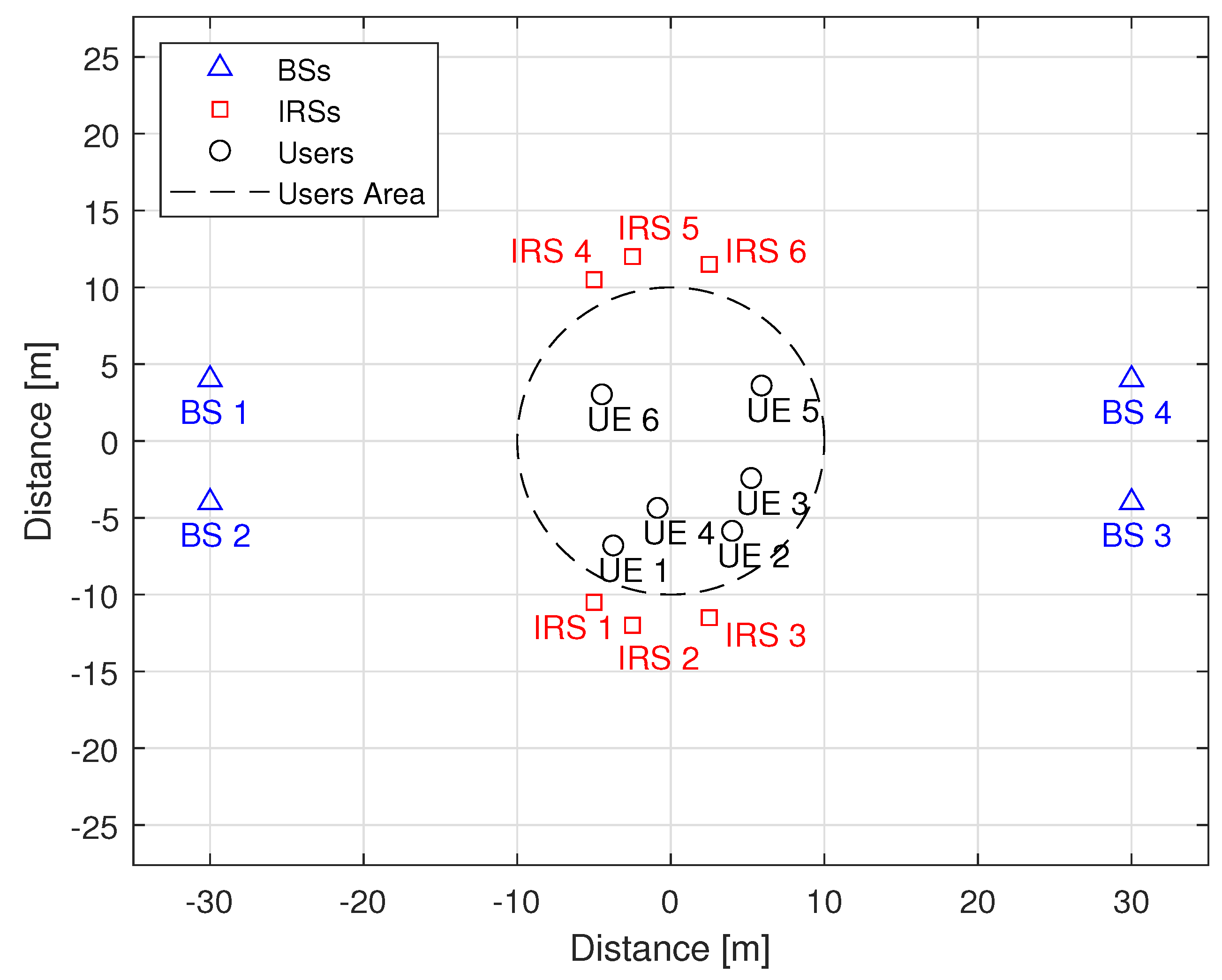
5. Simulation Results

In this section, we present the numerical results for the proposed algorithm under the continuous phases scenario and the discrete phases scenario. For the system parameters regarding the network deployment, we follow the latest relevant works in [14]. Figure 5 depicts the 2D deployment of the studied system, where four BSs are positioned by coordinates ( x s , y s , z s ) at (−30,4,5) [m], (−30,−4,5) [m], (30,−4,5) [m], and (30,4,5) [m], respectively. Additionally, six IRSs are positioned by coordinates denoted by ( x l , y l , z l ) as follows: (−5,−10.5,5) [m], (−2.5,−12,5) [m], (2.5,−11.5,5) [m], (−5,−10.5,5) [m], (−2.5,−12,5) [m], and (2.5,11.5,5) [m], respectively. These IRSs share the same BS height. A total of six UEs are distributed randomly along the circumference of a circle. Specifically, the circle is centered at (0,0) with a diameter of D = 20 [m] and positioned in front of the IRSs. We assume the UEs change their positions at the beginning of each episode. Following a random walk, each UE has a moving angle g k ( 0 g k 2 π ) and a moving speed v k ( 0 v k 1 ) [m/s] within the confined region, as depicted in Figure 5. In the simulations, we set 2 d l = 2 d s = λ c , N H = 1 for odd N, N H = 2 for even N, and increase N V at the IRSs. The path losses in the channels are expressed by the models 32.6 + 36.7 log 10 ( d direct ) [dB] [8] and 35.6 + 22 log 10 ( d indirect ) [dB] [8], respectively. Here, d direct represents the distance between the s-th BS and the k-th UE in the direct link, while d indirect signifies the corresponding distance between nodes in indirect links, namely the s-th BS to the l-th IRS or the l-th IRS to the k-th UE. Other simulation parameters include ε = 10, noise power σ k 2 = 80 [dBm] and R min = 1 [bps].
In the proposed cooperative MADRL framework, all DRL units, including DDPG and DQN units, are structured from FC-DNNs. Each network is composed of five layers, i.e., one input layer, one output layer, and two hidden layers, with a normalization layer in between to expedite convergence and reduce training time. The dimensions of the networks are contingent on the sizes of states and actions. We configure the hidden layer to be suitable for our studied system setup [21]. This configuration strikes a balance between model complexity and performance, as confirmed through empirical testing. In addition, Tanh and Relu models are applied as activation functions, chosen for their facilitation of gradient descent and backpropagation. To explore the action set in the DDPG algorithm, we introduce a complex Gaussian noise with zero mean and variance, i.e., σ 2 . Denote T s as the sampling time; accordingly, σ 2 · T s typically satisfy ( 1 % to 10 % ) of the range of the DDPG action. The remaining hyper-parameters are listed in Table 4. Part of these parameters is aligned with [21,31], while others are chosen through extensive trials.
To demonstrate the performance of the proposed algorithm, we compare it with benchmark schemes. The scenarios and benchmark schemes under consideration include:
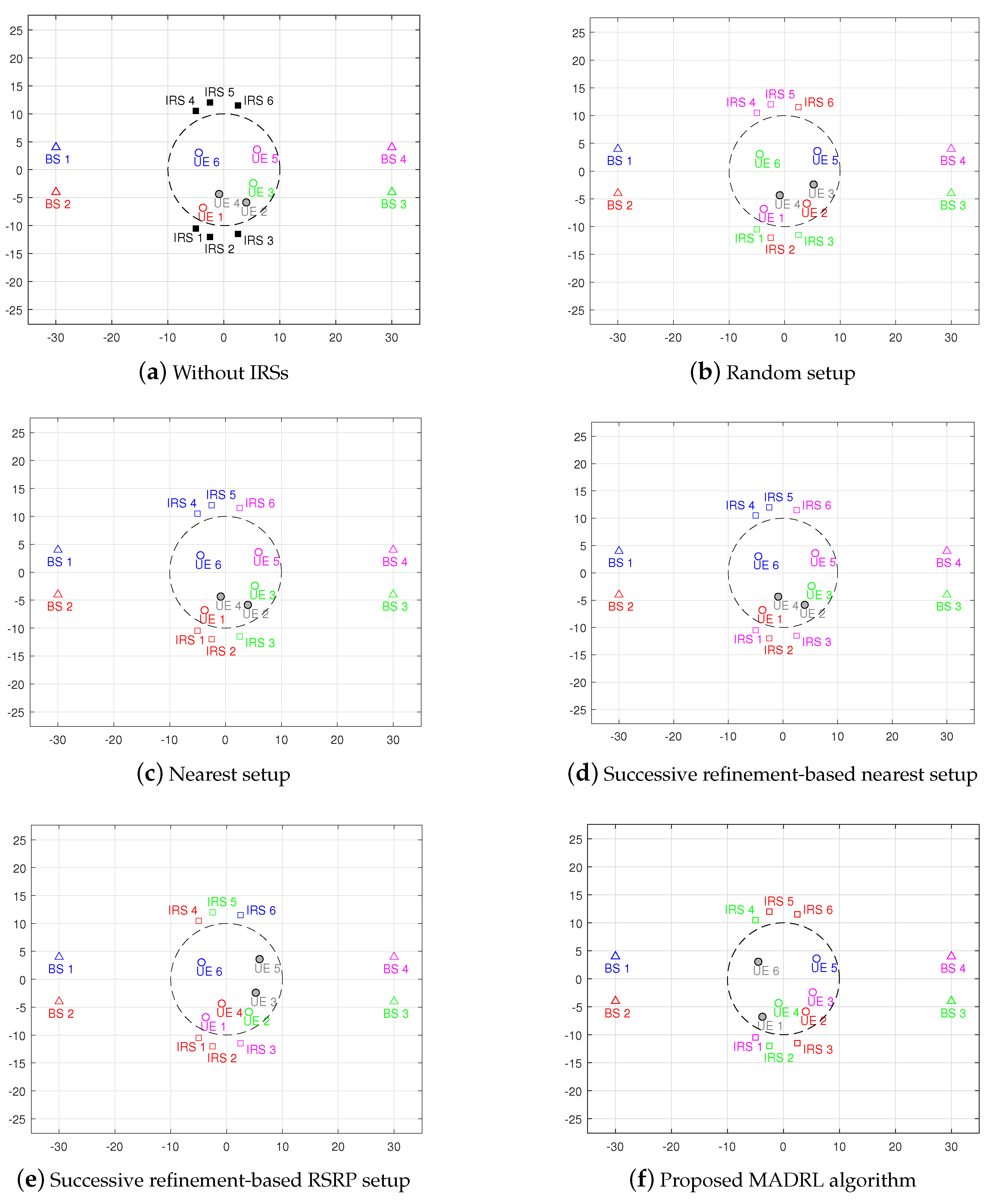
  • Without IRSs: conventional system without IRSs aid, i.e., switch off all the deployed IRSs and no related associations.
  • Random setup: system with the BS–IRS–UE associations are set up randomly.
  • Nearest setup: system with the BS–IRS–UE associations are set up based on the nearest association rule.
  • Successive refinement-based algorithm: system with the BS–IRS associations are set up based on the iterative successive refinement optimization algorithm [13,14].

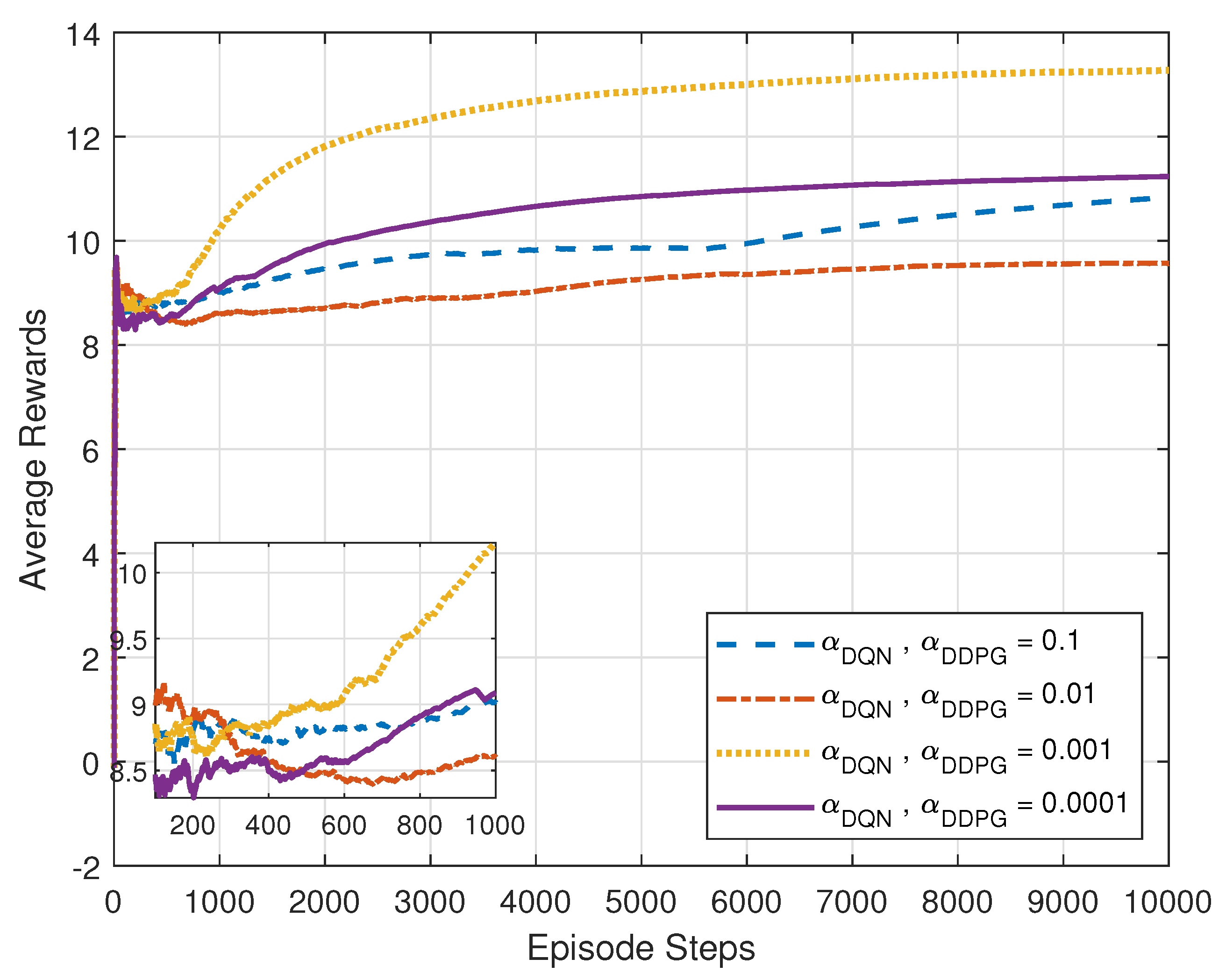
5.1. Performance Analysis of the Proposed MADRL-Based Algorithm

The proposed cooperative MADRL-based algorithm should be trained to yield high sum rates and output performance. Consequently, we monitor the network during episode steps’ training and investigate the effects of the learning rates and target smooth factors for both DQN and DDPG units. These parameters are considered critical hyper-parameters for the agents. It is important to note that we initially consider the continuous phases case to tune these parameters and then apply the tuned values to the discrete phases case.
Figure 6 plots the average reward versus the episode steps under various learning rates for the agents’ learning units. The average rewards are computed by accumulating instantaneous rewards over episode steps. It is observed that, for any given learning rate, agents initially receive low rewards. As the number of steps increases, these rewards grow until convergence to the episode occurs. This is primarily due to the fact that the relatively lower experience in the buffer during the early steps leads to a higher sample correlation and, consequently, poorer training performance for the agents. However, as experiences accumulate in the buffer, the agents collaborate to enhance the long-term rewards. Specifically, the figure illustrates that the curve attains the highest average rewards at a learning rate of 0.001. The improvement in performance resulting from the lower learning rate comes with the drawback of an extended convergence time. Additionally, it is worth noting that higher rates lead to increased oscillations, resulting in performance degradation. This implies that an optimal learning rate is necessary, as excessively low or high values may compromise both performance and convergence. Thus, we configure the learning rates for both DQN and DDPG units in all the agents to be 0.001, ensuring the optimization of long-term rewards and aligning with the main target of maximizing the system sum rate.
We also fine-tune the smoothing factor used in both DQN and DDPG units. Typically, it is necessary to set this value to less than 1 to ensure smoothness. In Figure 7, the average rewards are plotted against episode steps across various smooth factors. Observations reveal that utilizing a smooth value of 0.001 produces superior performance when compared to alternative values. Furthermore, it is observed that an increase in this value diminishes average rewards and degrades overall performance. This suggests that employing low smooth values for the agents is well-adapted for updating the target networks and converging towards optimal solutions for the studied system. Thus, we employ a smooth factor of 0.001 for both the DQN and DDPG units in all agents.
Figure 8 depicts the average total rewards achieved during total episodes with the adjusted parameters under both continuous and discrete cases. This average is determined by summing the cumulative values across all episodes. At the beginning of each episode, it is important to note that the environment undergoes a reset to assign new channel gains and UE positions. We assume a random walk for UEs, where each UE has a moving angle g k ( 0 g k 2 π ) and a moving speed v k ( 0 v k 1 ) [m/s] within the confined region, as depicted in Figure 5. The plot demonstrates that the average total achieved sum rate increases with the number of training episodes until convergence is achieved. This indicates that the agents update their policy after each episode, progressively optimizing toward the objective of maximizing the system sum rate under varying positions for UEs with different channel gains.

5.2. Performance Comparison of the Proposed MADRL-Based Algorithm under the Continuous Phases Case

In this subsection, we compare our proposed cooperative MADRL-based algorithm under the case of the continuous phases with the presented benchmark schemes regarding the optimized total sum rate of the served UEs.
Figure 9 plots the optimized sum instantaneous sum rate versus the BS maximum transmit power under different schemes, where UEs’ locations are generated from a single random realization, as illustrated in Figure 5. Note that all the benchmarks are enumerated on five discrete power levels to form a power space in the range P d = 0 , , p max .
From Figure 9, we note that our cooperative MADRL-based algorithm achieves the highest optimized sum rate compared to other benchmark schemes. This underscores the superiority of the proposed algorithm in reaching optimized values for the sum rate. The figure shows that the optimized sum rate is improved by increasing the BS maximum transmit power p max until it reaches a limit, where the power range of BS is consistent with [4,8,23,31]. Similar to a traditional network without IRSs-aid, this behavior arises from the potential increase in transmit power from the BSs, boost impacts the strength of both the desired signal and co-channel interference at the served UEs in a comparable manner. Consequently, the SINR experiences enhancement until reaching a limit as p max grows larger. In contrast, it is noted that with any given p max , well-optimizing the BS–IRS–UE associations can dramatically improve the optimized rate beyond the converged level. Contrasted with scenarios incorporating IRSs, the total achieved rate for the scenario without IRSs is the lowest because this scenario does not have the power gain due to the deployment of IRSs. In the conventional system without IRSs, the associations between BSs and UEs are set based on the nearest association rule. Then, the performance of the random setup scheme ranks as the second-worst. This indicates the importance of optimizing the BS–IRS–UE associations rather than randomly selecting them to maximize the benefits of IRS deployment. Applying the nearest association rule between system nodes enhances the sum rate compared to random associations. Moreover, when applying the successive refinement algorithm for optimizing the BS–IRS association, considering the BS–UE association based on nearest and RSRP setups, we can notice that the performance of the successive refinement algorithm-based RSRP is better than the successive refinement algorithm-based nearest. This is because, for any given configuration of IRS phases, the maximum RSRP association rule is a CSI-based association strategy that is determined by the strength of the UE received signal from both direct and indirect paths instead of distance-based association in the nearest setup. This is also well suited to the MRT active beamforming design in our system model. Concluding, we can find improved optimizations by applying the proposed algorithm, which jointly optimizes all optimization variables for maximizing the long-term sum rate.
Figure 10 plots the optimized BS–IRS–UE associations under different approaches for maximizing the sum rate at p max = 4 dBm. At each time step, the served UEs are marked by the same color as their associated BSs and IRSs, while the waiting UEs or those not served at this time step are marked in “gray”. Figure 11 shows the corresponding achieved system utility by the serving BSs. In Figure 10a, without the aid of IRSs, each BS serves the nearest UE. This has the lowest network utility compared to approaches with the IRS aid, with UE 3 and 6 identified as bottleneck users. In Figure 10b, with IRSs activated and random associations between nodes, some gains are observed, reflecting the impact of setting up the BS–IRS–UE associations to maximize the total network utility. In Figure 10c, associating the nearest IRSs to aid the transmission between the served UEs and their serving BSs enhances the rates of the bottleneck UEs in Figure 10a and increases the total sum rate.
In Figure 10d, the successive refinement algorithm-based nearest algorithm optimizes the BS–IRS association to maximize the achieved utility. The BS1–IRS association is kept the same, as it already achieved a high rate by serving UE6. To maximize the sum rate for other BSs and increase the achieved rates at their served UEs, re-association is performed, as shown in Figure 10d. For example, BS4 is associated with two extra-aiding IRSs to aid the transmission of the UE5. In Figure 10e, by re-associating the BS–UE based on RSRP instead of the nearest approach, the successive refinement algorithm demonstrates that it can increase the BSs’ sum rates. This is because RSRP considers the direct and indirect channel conditions between BSs and UEs, instead of just the distance, as in the nearest approach case. For example, BS4 serves UE1 instead of UE5, maximizing the utility of BS4. Note that the BS–UE in the RSRP-based association is determined based on the random phases for the IRSs, which may affect the optimal BS–UE with the instant CSI. Figure 10f plots the optimized BS–IRS–UE associations by applying the proposed MADRL-based algorithm, which led to maximizing the total achieved rates, as shown in Figure 11. This reflects that the agents work together over time to improve the association matrices and, as a result, fine-tuning the phases and the BSs’ power controls to maximize the overall system rate.
Figure 12 plots the optimized total average sum rate versus the number of elements per IRS in the continuous case for various schemes. Here, we average each simulated result over 100 random UE position initializations following their mobility model as described above, with a transmit power constraint of 0 dBm for each BS. The plot shows that the average achieved rate for the proposed algorithm increases with the growing number of IRS reflecting elements, surpassing the iterative successive refinement algorithm. This indicates that increasing the number of reflecting elements, along with well-optimized association design and power control, enhances the gains brought by these IRSs, thereby improving the utility of the source BSs. Furthermore, the random and nearest setup algorithms achieve comparable results and, notably, their performance degrades as N increases. This degradation is due to their static association design, which relies on the fixed locations of UEs.

5.3. Performance Comparison of the Proposed MADRL-Based Algorithm under the Discrete Phases Case

In this subsection, we compare our proposed cooperative MADRL-based algorithm under the case of the discrete phases with the considered benchmark schemes in terms of the total sum rate of the served UEs.
Figure 13 plots the optimized sum instantaneous achieved rate for the served UEs versus the BS maximum transmit power under different schemes. As shown in Figure 13, the proposed cooperative MADRL-based algorithm allows the achieved sum rate to reach high values compared with other approaches, indicating the effectiveness of the proposed algorithm. Similar to Figure 9, under the case of the discrete phases, a system not relying on assistance from IRSs results in the lowest achieved rate. Moreover, the achieved rate of applying random associations between system nodes is still constrained by the association design, which is enhanced when applying the nearest association setup algorithm. Finally, the successive refinement algorithm shows sub-optimal solutions that depend on the iterative process. In the benchmark schemes, it is important to highlight that the discrete phase shifts are determined by quantizing the continuous phase shifts obtained to their nearest values in F l . This quantization is expressed as θ l , n * = argmin θ F l θ θ l , n * , where θ l , n * is the optimal discrete phase shift of the n-th element at the l-th IRS.
Under the case of the discrete phases, Figure 14 depicts the optimized BS–IRS–UE associations under both the successive refinement and the proposed cooperative MADRL algorithm designed to maximize the sum rate. Note that we omit association figures for other approaches, since they are the same as those in Figure 10. Figure 15 illustrates the corresponding achieved sum rate by the serving BSs. As depicted, applying the proposed cooperative MADRL algorithm results in a higher achieved sum rate at the BSs. This verifies the superiority of our proposed approach over other benchmarks.
Figure 16 plots the optimized total average sum rate versus the number of elements per IRS under the case of the discrete phase for the optimizing schemes. We average each simulated result over 100 random UE position initializations, with a transmit power constraint of 0 dBm for each BS. Similar to Figure 12, it is observed that the average achieved rate for the proposed algorithm increases with the growing number of the IRSs reflecting units and exhibits the highest achieved sum rate compared to other schemes. The successive refinement algorithm shows the second-best performance. For comparison, the random and nearest setup algorithms also achieve comparable results, with minimal enhancement in their performance as N increases. This indicates that increasing the number of reflecting elements with well-optimized association design and power control enhances the gains brought by these IRSs, thereby helping the BSs improve the total sum rate.
Figure 17 plots the optimized total average sum rate versus the number of elements per IRS under different resolutions for different schemes. In this context, we specifically consider both b = 1 and b = 2 for discrete phase shifts at each IRS. Similarly, we average each simulated result over 100 random UE position initializations, with a transmit power constraint of 0 dBm for each BS. From the figure, it is observed that as N increases, the performance gap between the considered schemes widens with increasing resolutions. This trend comes from the fact that higher resolutions provide more flexibility in designing the phases of the IRSs, leading to an enhancement in the total sum rate.

6. Conclusions

In this work, we have investigated a large-scale communication system with multi-BS assisted by multi-IRS to serve multi-UE, where the joint optimization of BS power control, IRS beamforming configuration, and associations design was studied to maximize the total sum rate. The cooperative MADRL-based algorithm was proposed for joint optimization under continuous and discrete phase cases. The demonstrated capability of these approaches includes real-time predictions in various channel conditions with different UE locations, while ensuring performance meets predefined criteria. The fine-tuning was applied to the proposed models, ensuring robust stability and convergence with a focus on maximizing long-term objectives. Our simulation results revealed that the proposed algorithm outperformed the presented iterative benchmarks with regard to the sum rate.

Author Contributions

M.F.: Conceptualization, Methodology, Software, Validation, Formal analysis, and Writing—original draft; Z.F.: Supervision and Funding acquisition; J.G.: Conceptualization, Data curation, Writing—review and editing, Visualization and Project administration; M.S.A.: Investigation and Resources. All authors have read and agreed to the published version of the manuscript.

Funding

This work was supported in part by National Natural Science Foundation of China under Grant 62001029 and in part by Beijing Natural Science Foundation under Grant L202015.

Data Availability Statement

The data presented in this study are available on request from the corresponding author.

Conflicts of Interest

The authors declare no conflicts of interest.

References

  1. Saad, W.; Bennis, M.; Chen, M. A vision of 6G wireless systems: Applications, trends, technologies, and open research problems. IEEE Netw. 2019, 34, 134–142. [Google Scholar] [CrossRef]
  2. Gong, S.; Lu, X.; Hoang, D.T.; Niyato, D.; Shu, L.; Kim, D.I.; Liang, Y.C. Toward smart wireless communications via intelligent reflecting surfaces: A contemporary survey. IEEE Commun. Surv. Tutor. 2020, 22, 2283–2314. [Google Scholar] [CrossRef]
  3. Di Renzo, M.; Debbah, M.; Phan-Huy, D.T.; Zappone, A.; Alouini, M.S.; Yuen, C.; Sciancalepore, V.; Alexandropoulos, G.C.; Hoydis, J.; Gacanin, H.; et al. Smart radio environments empowered by reconfigurable AI meta-surfaces: An idea whose time has come. EURASIP J. Wirel. Commun. Netw. 2019, 2019, 129. [Google Scholar] [CrossRef]
  4. Wu, Q.; Zhang, R. Intelligent reflecting surface enhanced wireless network via joint active and passive beamforming. IEEE Trans. Wirel. Commun. 2019, 18, 5394–5409. [Google Scholar] [CrossRef]
  5. Hu, S.; Rusek, F.; Edfors, O. Beyond massive MIMO: The potential of data transmission with large intelligent surfaces. IEEE Trans. Signal Process. 2018, 66, 2746–2758. [Google Scholar] [CrossRef]
  6. Fu, M.; Zhou, Y.; Shi, Y. Intelligent reflecting surface for downlink non-orthogonal multiple access networks. In Proceedings of the 2019 IEEE Globecom Workshops (GC Wkshps), Waikoloa, HI, UA, 9–13 December 2019; IEEE: New York, NY, USA, 2019; pp. 1–6. [Google Scholar]
  7. Huang, C.; Zappone, A.; Alexandropoulos, G.C.; Debbah, M.; Yuen, C. Reconfigurable intelligent surfaces for energy efficiency in wireless communication. IEEE Trans. Wirel. Commun. 2019, 18, 4157–4170. [Google Scholar] [CrossRef]
  8. Guo, H.; Liang, Y.C.; Chen, J.; Larsson, E.G. Weighted sum-rate maximization for reconfigurable intelligent surface aided wireless networks. IEEE Trans. Wirel. Commun. 2020, 19, 3064–3076. [Google Scholar] [CrossRef]
  9. Li, Z.; Hua, M.; Wang, Q.; Song, Q. Weighted sum-rate maximization for multi-IRS aided cooperative transmission. IEEE Wirel. Commun. Lett. 2020, 9, 1620–1624. [Google Scholar] [CrossRef]
  10. Han, P.; Zhou, Z.; Wang, Z. Joint user association and passive beamforming in heterogeneous networks with reconfigurable intelligent surfaces. IEEE Commun. Lett. 2021, 25, 3041–3045. [Google Scholar] [CrossRef]
  11. Alwazani, H.; Nadeem, Q.U.A.; Chaaban, A. Performance Analysis under IRS-User Association for Distributed IRSs Assisted MISO Systems. arXiv 2021, arXiv:2111.02531. [Google Scholar]
  12. Zhao, D.; Lu, H.; Wang, Y.; Sun, H. Joint passive beamforming and user association optimization for IRS-assisted mmWave systems. In Proceedings of the GLOBECOM 2020—2020 IEEE Global Communications Conference, Taipei, Taiwan, 7–11 December 2020; IEEE: New York, NY, USA, 2020; pp. 1–6. [Google Scholar]
  13. Mei, W.; Zhang, R. Joint base station-IRS-user association in multi-IRS-aided wireless network. In Proceedings of the GLOBECOM 2020—2020 IEEE Global Communications Conference, Taipei, Taiwan, 7–11 December 2020; IEEE: New York, NY, USA, 2020; pp. 1–6. [Google Scholar]
  14. Mei, W.; Zhang, R. Performance analysis and user association optimization for wireless network aided by multiple intelligent reflecting surfaces. IEEE Trans. Commun. 2021, 69, 6296–6312. [Google Scholar] [CrossRef]
  15. Zhao, D.; Lu, H.; Wang, Y.; Sun, H.; Gui, Y. Joint power allocation and user association optimization for IRS-assisted mmWave systems. IEEE Trans. Wirel. Commun. 2021, 21, 577–590. [Google Scholar] [CrossRef]
  16. Taghavi, E.M.; Alizadeh, A.; Rajatheva, N.; Vu, M.; Latva-aho, M. User association in millimeter wave cellular networks with intelligent reflecting surfaces. In Proceedings of the 2021 IEEE 93rd Vehicular Technology Conference (VTC2021-Spring), Virtual Event, 25–28 April 2021; IEEE: New York, NY, USA, 2021; pp. 1–6. [Google Scholar]
  17. Liu, Y.; Liu, X.; Mu, X.; Hou, T.; Xu, J.; Di Renzo, M.; Al-Dhahir, N. Reconfigurable intelligent surfaces: Principles and opportunities. IEEE Commun. Surv. Tutor. 2021, 23, 1546–1577. [Google Scholar] [CrossRef]
  18. Taha, A.; Zhang, Y.; Mismar, F.B.; Alkhateeb, A. Deep reinforcement learning for intelligent reflecting surfaces: Towards standalone operation. In Proceedings of the 2020 IEEE 21st International Workshop on Signal Processing Advances in Wireless Communications (SPAWC), Atlanta, GA, USA, 26–29 May 2020; IEEE: New York, NY, USA, 2020; pp. 1–5. [Google Scholar]
  19. Taha, A.; Alrabeiah, M.; Alkhateeb, A. Enabling large intelligent surfaces with compressive sensing and deep learning. IEEE Access 2021, 9, 44304–44321. [Google Scholar] [CrossRef]
  20. Zhang, Q.; Saad, W.; Bennis, M. Millimeter wave communications with an intelligent reflector: Performance optimization and distributional reinforcement learning. IEEE Trans. Wirel. Commun. 2021, 21, 1836–1850. [Google Scholar] [CrossRef]
  21. Huang, C.; Mo, R.; Yuen, C. Reconfigurable intelligent surface assisted multiuser MISO systems exploiting deep reinforcement learning. IEEE J. Sel. Areas Commun. 2020, 38, 1839–1850. [Google Scholar] [CrossRef]
  22. Yang, H.; Xiong, Z.; Zhao, J.; Niyato, D.; Xiao, L.; Wu, Q. Deep reinforcement learning-based intelligent reflecting surface for secure wireless communications. IEEE Trans. Wirel. Commun. 2020, 20, 375–388. [Google Scholar] [CrossRef]
  23. Liu, X.; Liu, Y.; Chen, Y.; Poor, H.V. RIS enhanced massive non-orthogonal multiple access networks: Deployment and passive beamforming design. IEEE J. Sel. Areas Commun. 2020, 39, 1057–1071. [Google Scholar] [CrossRef]
  24. Fathy, M.; Fei, Z.; Guo, J.; Abood, M.S. Machine-Learning-Based Optimization for Multiple-IRS-Aided Communication System. Electronics 2023, 12, 1703. [Google Scholar] [CrossRef]
  25. Fathy, M.; Abood, M.S.; Guo, J. A Generalized Neural Network-based Optimization for Multiple IRSs-aided Communication System. In Proceedings of the 2021 IEEE 21st International Conference on Communication Technology (ICCT), Tianjin, China, 13–16 October 2021; IEEE: New York, NY, USA, 2021; pp. 480–486. [Google Scholar]
  26. Ahsan, W.; Yi, W.; Qin, Z.; Liu, Y.; Nallanathan, A. Resource allocation in uplink NOMA-IoT networks: A reinforcement-learning approach. IEEE Trans. Wirel. Commun. 2021, 20, 5083–5098. [Google Scholar] [CrossRef]
  27. Zhang, Y.; Mou, Z.; Gao, F.; Jiang, J.; Ding, R.; Han, Z. UAV-enabled secure communications by multi-agent deep reinforcement learning. IEEE Trans. Veh. Technol. 2020, 69, 11599–11611. [Google Scholar] [CrossRef]
  28. Zhong, R.; Liu, X.; Liu, Y.; Chen, Y. Multi-agent reinforcement learning in NOMA-aided UAV networks for cellular offloading. IEEE Trans. Wirel. Commun. 2021, 21, 1498–1512. [Google Scholar] [CrossRef]
  29. Omidshafiei, S.; Pazis, J.; Amato, C.; How, J.P.; Vian, J. Deep decentralized multi-task multi-agent reinforcement learning under partial observability. In Proceedings of the International Conference on Machine Learning, Sydney, Australia, 6–11 August 2017; PMLR: Baltimore, MA, USA, 2017; pp. 2681–2690. [Google Scholar]
  30. Nasir, Y.S.; Guo, D. Multi-agent deep reinforcement learning for dynamic power allocation in wireless networks. IEEE J. Sel. Areas Commun. 2019, 37, 2239–2250. [Google Scholar] [CrossRef]
  31. Chen, J.; Guo, L.; Jia, J.; Shang, J.; Wang, X. Resource allocation for IRS assisted SGF NOMA transmission: A MADRL approach. IEEE J. Sel. Areas Commun. 2022, 40, 1302–1316. [Google Scholar] [CrossRef]
  32. Huang, C.; Chen, G.; Wong, K.K. Multi-agent reinforcement learning-based buffer-aided relay selection in IRS-assisted secure cooperative networks. IEEE Trans. Inf. Forensics Secur. 2021, 16, 4101–4112. [Google Scholar] [CrossRef]
  33. Pan, C.; Ren, H.; Wang, K.; Elkashlan, M.; Nallanathan, A.; Wang, J.; Hanzo, L. Intelligent reflecting surface aided MIMO broadcasting for simultaneous wireless information and power transfer. IEEE J. Sel. Areas Commun. 2020, 38, 1719–1734. [Google Scholar] [CrossRef]
  34. Jiang, T.; Cheng, H.V.; Yu, W. Learning to reflect and to beamform for intelligent reflecting surface with implicit channel estimation. IEEE J. Sel. Areas Commun. 2021, 39, 1931–1945. [Google Scholar] [CrossRef]
  35. Grant, M.; Boyd, S. CVX: Matlab Software for Disciplined Convex Programming, Version 2.2. 2020. Available online: http://cvxr.com/cvx/ (accessed on 22 January 2024).
  36. 3GPP TR 38.901. Study on Channel Model for Frequencies from 0.5 to 100 GHz. 2017. Available online: https://portal.3gpp.org/desktopmodules/Specifications/SpecificationDetails.aspx?specificationId=3173 (accessed on 20 March 2023).
  37. Sutton, R.S.; Barto, A.G. Introduction to Reinforcement Learning; BooksRun: Philadelphia, PA, USA, 2018. [Google Scholar]
  38. Sur, S.N.; Singh, A.K.; Kandar, D.; Silva, A.; Nguyen, N.D. Intelligent Reflecting Surface Assisted Localization: Opportunities and Challenges. Electronics 2022, 11, 1411. [Google Scholar] [CrossRef]
  39. Melo, F.S. Convergence of Q-Learning: A Simple Proof; Technical Report; Institute of Systems and Robotics, 2001; pp. 1–14. Available online: https://www.academia.edu/download/55970511/ProofQlearning.pdf (accessed on 20 March 2023).
  40. Timofte, V.; Timofte, A.; Khan, L.A. Stone–Weierstrass and extension theorems in the nonlocally convex case. J. Math. Anal. Appl. 2018, 462, 1536–1554. [Google Scholar] [CrossRef]
  41. Yang, Z.; Liu, Y.; Chen, Y.; Al-Dhahir, N. Machine learning for user partitioning and phase shifters design in RIS-aided NOMA networks. IEEE Trans. Commun. 2021, 69, 7414–7428. [Google Scholar] [CrossRef]
  42. Burkard, R.; Dell’Amico, M.; Martello, S. Assignment Problems: Revised Reprint; SIAM: Philadelphia, PA, USA, 2012. [Google Scholar]
Figure 1. Architecture of multi-IRS-aided multi-BS communication system.
Electronics 13 00735 g001
Figure 2. Proposed MADRL-based frameworks under IRS configurations cases.
Electronics 13 00735 g002
Figure 3. DRL units architecture: (a) DQN unit; (b) DDPG unit.
Electronics 13 00735 g003
Figure 4. Flow chart of the proposed MADRL-based algorithm.
Electronics 13 00735 g004
Figure 5. 2D−system deployment.
Electronics 13 00735 g005
Figure 6. Average rewards versus episode steps with various learning rates.
Electronics 13 00735 g006
Figure 7. Average rewards versus episode steps with various target smoothing factors.
Electronics 13 00735 g007
Figure 8. Average rewards versus versus learning episodes.
Electronics 13 00735 g008
Figure 9. Optimized instantaneous sum rate versus BS maximum transmit power for different approaches under continuous phases.
Electronics 13 00735 g009
Figure 10. Optimized BS–IRS–User associations under continuous phases case for different approaches: (a) without IRSs; (b) random setup; (c) nearest setup; (d) successive refinement-based nearest setup; (e) successive refinement-based RSRP setup; (f) proposed MADRL algorithm.
Electronics 13 00735 g010
Figure 11. Optimized sum rate versus different approaches under continuous phases case.
Electronics 13 00735 g011
Figure 12. Optimized average sum rate versus number of reflecting elements for different approaches under continuous phases.
Electronics 13 00735 g012
Figure 13. Optimized instantaneous sum rate versus BS maximum transmit power for different approaches under discrete phases.
Electronics 13 00735 g013
Figure 14. Optimized BS–IRS–User associations under discrete phases case for different approaches: (a) successive refinement-based RSRP setup; (b) proposed MADRL algorithm.
Electronics 13 00735 g014
Figure 15. Optimized sum rate versus different approaches under discrete phases case.
Electronics 13 00735 g015
Figure 16. Optimized average sum rate versus number of reflecting elements for different approaches under discrete phases.
Electronics 13 00735 g016
Figure 17. Optimized average sum rate versus number of reflecting elements for different approaches under discrete phases with different resolutions.
Electronics 13 00735 g017
Table 1. Implementation complexity comparison.
ApproachComplexity
Exhaustive Approach O ( S K + L )
Graph-theoretic Algorithm O ( K · S 2 ) [42]
Successive Refinement Algorithm O ( I t · K · S 3 ) [13,14]
Proposed MADRL Algorithm (continuous) O ( P ( L , N , M , K , n ) )
Proposed MADRL Algorithm (discrete) O ( P ( L , N , M , K , B , S , n ) )
Table 2. Average implementation run-time (seconds) under continuous phases case.
N5101520
Algorithm
Successive Refinement Algorithm44.663778.5485120.3662153.0799
Proposed MADRL Algorithm0.43720.43800.44240.4669
Table 3. Average implementation run-time (seconds) under discrete phases case.
N5101520
Algorithm
Successive Refinement Algorithm80.854994.6200101.2413134.2253
Proposed MADRL Algorithm0.44781.250538.94291050
Table 4. Proposed MADRL framework hyper-parameters settings.
Hyper-ParameterSetting
Learning rates α DQN , α DDPG 0.001
Discount factor γ 0.95
Buffer size C200,000
Mini-batch size N B 16
Probability threshold ϵ 1
Min Probability threshold ϵ min 0.01
Decay rate α decay 0.0050
Target smooth factors τ DQN , τ DDPG 0.001
Target update frequency U1
Sampling time T s 1
Disclaimer/Publisher’s Note: The statements, opinions and data contained in all publications are solely those of the individual author(s) and contributor(s) and not of MDPI and/or the editor(s). MDPI and/or the editor(s) disclaim responsibility for any injury to people or property resulting from any ideas, methods, instructions or products referred to in the content.

