Design of Multivariable PID Control Using Iterative Linear Programming and Decoupling

Abstract

The design of multivariable process control systems is specially complicated when there are strong interactions between the different control loops, and even more with multiple time delays. This paper proposes an iterative design method of centralized proportional-integral-derivative (PID) controllers for stable linear systems. The methodology is based on the linear parameterization of equivalent loop transfer functions (ELTFs) for centralized control. These functions capture the dynamics of the other loops and, from a prior design, allow solving the design problem at each iteration with linear programming that shapes the Nyquist plot of the ELTFs in the frequency domain, which also avoids the need for approximations. Two optimizations are proposed: (I) maximizing integral gains by fulfilling linear robustness margins in each ELTF and (II) maximizing linear robustness margins by fulfilling minimum bandwidths in each loop. In both optimizations, static decoupling and decoupling at a frequency close to the bandwidth of each loop are included as constraints, which improves the decoupling performance and the procedure convergence. The effectiveness of the method is verified in three simulation examples (square and non-square) and a lab experimental process. The proposed designs achieve a similar or better response when compared to that achieved by other authors.

1. Introduction

For decades, proportional-integral-derivative (PID) controllers have been the most widespread in industrial processes, where it is estimated that they are currently present in 90% of control loops due to their efficiency and simplicity of implementation [1]. Although predictive control (MPC) is now more widespread in the industry, its bandwidth limitations mean that in the regulation layer, PID controllers are still preferred, with MPC being implemented in a higher layer [2]. PID controller tuning methods are mainly developed for single-variable loops [3,4]. However, most industrial processes are multivariable and have multiple inputs and multiple outputs (MIMOs). For the performance of these systems not to deteriorate, the possible interaction between the inputs and outputs of the process or their possible multiple time delays must be considered. These aspects render these systems more difficult to control and render the design of MIMO control systems more complicated than in the single-variable case [5]. To deal with multivariable systems, there are two main approaches: multiloop (or decentralized) control and centralized control.

In multiloop control, the MIMO system is decomposed into several single-variable loops where each output is paired with an input and a controller is designed for each loop, usually a PID controller [6,7]. The resulting control is a diagonal matrix controller. There are different methods for its design, such as detuning, the sequential loop closing method [8], optimization [9,10], direct design [6], or an iterative method based on the concept of effective open loop processes and robustness specifications in the frequency domain [11,12]. In cases with less interaction, even PID SISO design methods [13,14] can be directly used. These approaches work well for weakly coupled processes but may be inadequate for highly interacting and diagonally nondominant processes. In these cases, the centralized control approach is more advisable, which can be realized either by combining a decoupler with a diagonal controller [15] or by designing a full matrix controller from the above blocks or directly [16,17].

In the purely centralized scheme, the full matrix controller is the only block responsible for reducing the interactions and controlling the different outputs of the system. The design of these controls can be approached with non-PID elements in the controller matrix and using different methods such as decoupling control [18], optimization procedures [19], H_∝ design [20], and so on. The resulting controllers can be highly complex and even irrational; therefore, several authors have subsequently proposed to approximate the elements of these controls to the PID structure [21], thus obtaining multivariable PID control. Other methodologies have been developed to directly obtain a complete matrix of PID controllers.

There is a large body of work on multivariable PID control design [22] in both the time and frequency domain. Among the design methods in the time domain, iterative methods based on linear matrix inequalities (LMIs) stand out [23,24,25]. However, in the case of systems with multiple time delays, the design of PID controllers can become difficult; therefore, frequency domain-based techniques are often used [2]. Several methods use a matrix representation of transfer functions and attempt to obtain an approximation of equivalent transfer functions (ETFs) to design multivariable PID controls [26,27]. In [28], the approximate ETFs are derived from the effective relative gain array (RGA) of the process. In [29], ETFs were obtained from the relative normalized gain array (RNGA), which approximates the inverse of the process matrix. In [30], they are calculated from the RGA and the average residence time array. Most centralized control methods are designed for square systems, where the number of process inputs and outputs is the same. For non-square systems, the design can be complicated by the uniqueness of the transfer function matrix of the process. One option is to create the process square by adding or removing the input or output variables. Adding outputs impacts the cost of measurement instrumentation, and removing inputs changes the properties of the original system [31]. In [32], the ETF concept was extended to non-square systems and proposed multivariable PID control with optimization via particle swarm optimization. In [33], the design method based on ETFs and the RNGA was extended to non-square systems.

Methods based on transfer functions or ETFs tend to become conservative when the process size increases because they require different approximations. To avoid these approximations, some authors have used internal model control [34] or proposed an LMI-based optimization [35]. On the other hand, other authors have avoided approximations during their design by directly working with the matrix representation of the process frequency response and using frequency domain specifications. In [36], the controller was designed using the process response at low frequencies to approximate the closed-loop response to that of a reference model. The method was presented for non-square systems based on the pseudoinverse evaluation of the process transfer function matrix at a low-frequency point. In [37], the frequency response was used to retune a PID MIMO controller. Other works [2,38] proposed the design of centralized PID control based on the frequency response of the process as a convex optimization problem with LMIs.

In our previous paper [39], we proposed an iterative method to design multivariable PID controls for stable and square linear systems based on their frequency response and the concept of equivalent loop transfer function (ELTF). In that study, ELTFs enabled the calculation of the elements for each column of the controller matrix separately using a linear optimization problem if the linear margin proposed in [40] was used as a robustness specification. Such a margin ensures the minimum values of other well-known margins, such as gain margin, phase margin, or maximum sensitivity. Moreover, such a method does not require any approximation when using the frequency response representation. In this paper, we present a new iterative multivariable PID control design methodology based on the previous one, which is extended. Now, instead of designing each column of the controller matrix separately, the entire design is performed in each iteration in a single linear programming problem. For this purpose, the ELTFs are expressed as a function of all the elements of the controller matrix. Thus, a better convergence is sought. In addition to static decoupling, which reduces the interaction at low frequencies, we add the option of including a dynamic decoupling constraint in each loop at a specific frequency close to the desired bandwidth, which helps to render the resulting system diagonally nondominant without imposing such strong constraints as full dynamic decoupling. In the previous study, the optimization problem maximized the integral gains subject to given robustness values; now, the optimization is also posed to maximize the linear robustness margins of each loop while ensuring the given bandwidths. The effectiveness of the method is verified via a simulation of two square linear processes with time delays with dimensions of 2 × 2 and 3 × 3 and a non-square 2 × 3 system. The proposed methods are also tested on a real quadruple tank process. Comparison with other authors shows that the proposed methodologies achieve a similar or better performance.

The rest of the article is as follows: Section 2 presents the linear robustness margin and the concept of an ETLF in centralized control. Section 3 describes the proposed methodology, explaining the different types of linear programming according to the cost function to be maximized and the different constraints to which it may be subject. In Section 4, the proposed method is applied to different processes and compared with controllers developed by other authors. Finally, Section 5 summarizes the main conclusions.

2. Preliminaries

Figure 1 shows a centralized unitary feedback control system in which the linear multivariable process is represented by the transfer function matrix G(s) of the dimension n × m and the centralized control by the matrix K(s) of m × n dimensions. When the number of outputs and inputs of the process is the same, these matrices are square. Each element g_ij(s) of G(s) represents the transfer function between output y_i and input u_j. Each controller k_ij(s) represents the control element between the control signal u_i and the error signal e_j, which is the difference between the reference signal r_j and the controlled output y_j. The open-loop transfer matrix is denoted as L(s) = G(s)K(s) when unitary feedback is assumed. In the 2 × 2 case, the elements l_ij(s) are provided in (1), where the Laplace variable s has been omitted, as shown in Figure 1. The elements of a single column of L(s) depend on the elements of a single column of K(s). Something similar happens for higher dimensional processes. Thus, for example, the generic element l_ij(s) of the j-th column of L(s) for n × n processes are provided with (2) and depends on the elements of the j-th column of K(s).

$$L=G·K=\left(\begin{array}{cc}{g}_{11}& g_{12}\\ g_{21}& g_{22}\end{array}\right)\left(\begin{array}{cc}{k}_{11}& k_{12}\\ k_{21}& k_{22}\end{array}\right)=\left(\begin{array}{cc}{g}_{11}{k}_{11}+g_{12}{k}_{21}& g_{11}{k}_{12}+g_{12}{k}_{22}\\ g_{21}{k}_{11}+g_{22}{k}_{21}& g_{21}{k}_{12}+g_{22}{k}_{22}\end{array}\right)=\left(\begin{array}{cc}{l}_{11}& l_{12}\\ l_{21}& l_{22}\end{array}\right)$$

(1)

$$l_{ij}(s)={\displaystyle \sum _{k=1}^m{g}_{ik}(s)k_{kj}(s)}$$

(2)

The problem with these open-loop transfer functions is that they do not capture the interactions and dynamics with the other loops when they are closed. In [39], the concept of an equivalent open-loop transfer function (ELTF) for centralized control was introduced. This function represents the transfer function between an output and its error signal when the loop is open and the rest of the loops remain closed. Figure 2 shows the ELTF l₁(s) framed for the 2 × 2 case. Unlike the l_ij(s) functions in L(s), the ELTF incorporates the interactions and dynamics with the other control loops. For the case with two outputs, the expressions of the ELTFs are shown in (3). For n dimensions, the generic expression is provided in (4).

$$l_1(s)=l_{11}(s)-\frac{l_{12}(s)l_{21}(s)}{1+l_{22}(s)}\hspace{1em}\hspace{1em}{l}_2(s)=l_{22}(s)-\frac{l_{21}(s)l_{12}(s)}{1+l_{11}(s)}$$

(3)

$$l_j(s)=l_{jj}(s)-{\displaystyle \sum _{\begin{array}{l}i=1\\ i\ne j\end{array}}^n\frac{l_{ij}(s)l_{ji}(s)}{1+l_{ii}(s)}}$$

(4)

As demonstrated in [39], ELTFs can be expressed as a function of controllers in the same column, which can be designed in isolation in an iterative process if the other control columns are known. By using PID controllers with parallel structures and linear robustness margins as a design specification for the frequency response of the ELTFs, this problem was posed as linear programming for each ELTF. The linear margin L_m is shown in Figure 3, where it is determined via the straight line r intercepting the negative real axis at the point (−1 + L_m, 0) with an angle α. If the ELTF l_i(s) is stable, closed-loop stability is guaranteed if its Nyquist trace is below the r-straight line because it does not encircle the critical point −1. Using the frequency response l_i(jω), where ω is the frequency variable, this condition can be expressed with the inequation shown in (5), where ℑ() represents the imaginary part, ℜ() is the real part, and tan() is the tangent function. Furthermore, as the polar trace lies below the line r, the minimum values of other classical robustness margins, such as gain margin A_m, phase margin ϕ_m, or maximum sensitivity margin M_s, all depicted in Figure 3, are guaranteed. More details on the relationship between these classical robustness margins and the values of L_m and α can be found in [39,40]. The robustness increases with increasing values of L_m and α, with typical ranges of [0.5, 0.85] for L_m and [35°, 90°] for α. Moreover, the higher these values are, the more damped the system will be and the lower the control effort will be; however, as a trade-off, the bandwidth decreases, which tends to render the settling time of the time response longer.

$$\Im \left(l_i(j{\omega }_k)\right)-\tan \alpha \left(\Re \left(l_i(j{\omega }_k)\right)+1-L_m\right)\le 0\hspace{1em}\forall {\omega }_k$$

(5)

In addition, Figure 3 shows the line q, which is tangential to the unit circle in the third quadrant and intercepts the negative real semi-axis with an angle β. With this line, a condition can be established on l_i(jω) to ensure a lower limit ω_x at the crossover frequency ω_c, which marks the bandwidth of the loop. Such a condition is provided in the inequations in (6): the first forces the trace of l_i(jω) to be below line q for frequencies lower than ω_x, and the second forces the trace at higher frequencies to be above line q. Here, cos and sin are the sine and cosine functions, respectively.

$$\begin{array}{ll}\cos {\beta }_j\Im \left(l_j(j{\omega }_k)\right)+\sin {\beta }_j\Re \left(l_j(j{\omega }_k)\right)\le -1& \forall {\omega }_k\le {\omega }_x\\ -\cos {\beta }_j\Im \left(l_j(j{\omega }_k)\right)-\sin {\beta }_j\Re \left(l_j(j{\omega }_k)\right)>-1& \forall {\omega }_k>{\omega }_x\end{array}$$

(6)

3. Proposed Methodology

This section describes the proposed iterative method for the design of MIMO PID controllers based on the frequency response of the ELTFs and the linear margin. The proposed method performs the design of all PID controllers in each iteration and not separately by columns, as in our previous work [39]; moreover, the linear programming developed for its resolution is proposed with different cost functions and constraints.

3.1. Linear Parameterization of ELTFs

The proposed method is based on a linear parameterization of the ELTFs as a function of the PID controller parameters. Assuming a parallel PID structure in the controller matrix K(s), the controllers have the form provided in (7), where K_Pij is the proportional gain of the control element kij(s), K_Iij is the integral gain, and K_Dij is the derivative gain. These can be linearly parameterized as a function of the parameter vector ρ_ij with the above gains, as shown in (7).

$$k_{ij}(s)=K_{Pij}+\frac{K_{Iij}}{s}+K_{Dij}s=\left[1,\frac{1}{s},s\right]\left[\begin{array}{c}{K}_{Pij}\\ K_{Iij}\\ K_{Dij}\end{array}\right]=\left[1,\frac{1}{s},s\right]{\mathsf{\rho }}_{ij}$$

(7)

We defined a vector ρ with all the parameters of all the K(s) controllers ordered by rows as shown in (8) for the 2 × 2 case.

$$\mathsf{\rho }={\left(\begin{array}{cc}\begin{array}{cc}{\mathsf{\rho }}_{11}^T& {\mathsf{\rho }}_{12}^T\end{array}& \begin{array}{cc}{\mathsf{\rho }}_{21}^T& {\mathsf{\rho }}_{22}^T\end{array}\end{array}\right)}^T$$

(8)

We defined the product of a process element g_km(s) by a controller element k_ij(s), as shown in (9), where the vector φ_km(s) encompasses the process element g_km(s) and the vector [1, 1/s, s] associated with the PID element. This product was linearly parameterized with respect to the PID parameter vector ρ_ij and the three-element row vector φ_km(s). For the elements of this vector, a priori, to be positive elements, the corresponding sign was extracted. The signs of the controller elements were obtained, assuming that the centralized control matrix K(s) at low frequencies would be proportional to the inverse (or pseudoinverse) of the steady-state process matrix, i.e., G(0). In fact, the sign was extracted so that the integral gains K_Iij were positive since they were forced to be positive in the subsequent optimization. After optimization, the sign corresponding to each controller k_ij(s) was returned. The sign function is represented by sign().

$$g_{km}(s)k_{ij}(s)=sign(k_{ij})g_{km}(s)\left[1,\frac{1}{s},s\right]\left[\begin{array}{c}{K}_{Pij}\\ K_{Iij}\\ K_{Dij}\end{array}\right]=sign(k_{ij})\left[g_{km}(s),\frac{g_{km}(s)}{s},s·g_{km}(s)\right]{\mathsf{\rho }}_{ij}={\mathsf{\phi }}_{km}(s){\mathsf{\rho }}_{ij}$$

(9)

From the latter expression, expressed the elements of the matrix L(s) as a linear parameterization of the total PID parameter vector ρ with the row vectors Λ_ij(s), which captured the process dynamics corresponding to l_ij(s) and the part in s of the PID controllers. Thus, for the 2 × 2 case, provided with the vector ρ in (8), the elements of L(s) in (1) could be compactly expressed as follows in (10), where Λ_ij(s) and ρ are 12-element vectors. For 3 × 3 or higher cases, a similar procedure could be followed to finally have any element of L(s) linearly parameterized with respect to the vector ρ of the PID parameters as l_ij(s) = Λ_ij(s)ρ.

$$\begin{array}{l}L(s)=\left(\begin{array}{cc}{g}_{11}(s)k_{11}(s)+g_{12}(s)k_{21}(s)& g_{11}(s)k_{12}(s)+g_{12}(s)k_{22}(s)\\ g_{21}(s)k_{11}(s)+g_{22}(s)k_{21}(s)& g_{21}(s)k_{12}(s)+g_{22}(s)k_{22}(s)\end{array}\right)=\\ =\left(\begin{array}{cc}\left[\begin{array}{cc}\begin{array}{cc}{\mathsf{\phi }}_{11}(s)& 0_{1x3}\end{array}& \begin{array}{cc}{\mathsf{\phi }}_{12}(s)& 0_{1x3}\end{array}\end{array}\right]\mathsf{\rho }& \left[\begin{array}{cc}\begin{array}{cc}{0}_{1x3}& {\mathsf{\phi }}_{11}(s)\end{array}& \begin{array}{cc}{0}_{1x3}& {\mathsf{\phi }}_{12}(s)\end{array}\end{array}\right]\mathsf{\rho }\\ \left[\begin{array}{cc}\begin{array}{cc}{\mathsf{\phi }}_{21}(s)& 0_{1x3}\end{array}& \begin{array}{cc}{\mathsf{\phi }}_{22}(s)& 0_{1x3}\end{array}\end{array}\right]\mathsf{\rho }& \left[\begin{array}{cc}\begin{array}{cc}{0}_{1x3}& {\mathsf{\phi }}_{21}(s)\end{array}& \begin{array}{cc}{0}_{1x3}& {\mathsf{\phi }}_{22}(s)\end{array}\end{array}\right]\mathsf{\rho }\end{array}\right)=\left(\begin{array}{cc}{\Lambda }_{11}(s)\mathsf{\rho }& {\Lambda }_{12}(s)\mathsf{\rho }\\ {\Lambda }_{21}(s)\mathsf{\rho }& {\Lambda }_{22}(s)\mathsf{\rho }\end{array}\right)\end{array}$$

(10)

From these parameterizations of the open-loop elements l_ij(s), the ELTFs could be expressed as a linear parameterization of the PID parameter vector, assuming that some functions of L(s) are previously known. For example, given the generic ELTF expression l_j(s) provided in (4), in the summation terms, the denominator 1 + l_ii(s) must be assumed to be previously known from a previous design, as well as one of the two elements of the numerator product. For instance, with the expressions in (3) for the 2 × 2 case, the ELTF l₁(s) could be parameterized as shown in (11), where the functions l₂₂(s) and l₁₂(s) are assumed to be known and where Ψ_1a(s) is a 12-element row vector. In this case, the columns of Ψ_1a(s) corresponding to the parameters of k₁₂ and k₂₂ are zeros, then l₁(s) is parameterized as a function of only the parameters of the controllers in column 1 of K(s), which would be the vectors ρ₁₁ and ρ₂₁. However, l₁(s) could also be expressed as in (12) if, instead of assuming l₁₂(s) to be known, l₂₁(s) is assumed to be known. In this case, l₁(s) depends on all controllers of K(s), i.e., on all the elements of ρ. For this case, we used the nomenclature Ψ_1b(s). For l₂(s), a similar parameterization could also be performed with two options. Using these two ways of representing the ELTFs allows better convergence in the subsequently proposed iterative process.

$$\begin{array}{l}{l}_1(s)=l_{11}(s)-\frac{l_{12}(s)l_{21}(s)}{1+l_{22}(s)}=\left({\Lambda }_{11}(s)-{\Lambda }_{21}(s)\frac{l_{12}(s)}{1+l_{22}(s)}\right)\mathsf{\rho }=\\ =\left(\left[\begin{array}{cc}\begin{array}{cc}{\mathsf{\phi }}_{11}(s)& 0_{1x3}\end{array}& \begin{array}{cc}{\mathsf{\phi }}_{12}(s)& 0_{1x3}\end{array}\end{array}\right]-\left[\begin{array}{cc}\begin{array}{cc}{\mathsf{\phi }}_{21}(s)& 0_{1x3}\end{array}& \begin{array}{cc}{\mathsf{\phi }}_{22}(s)& 0_{1x3}\end{array}\end{array}\right]\frac{l_{12}(s)}{1+l_{22}(s)}\right)\mathsf{\rho }={\Psi }_{1a}(s)\mathsf{\rho }\end{array}$$

(11)

$$\begin{array}{l}{l}_1(s)=l_{11}(s)-\frac{l_{12}(s)l_{21}(s)}{1+l_{22}(s)}=\left({\Lambda }_{11}(s)-{\Lambda }_{12}(s)\frac{l_{21}(s)}{1+l_{22}(s)}\right)\mathsf{\rho }=\\ =\left(\left[\begin{array}{cc}\begin{array}{cc}{\mathsf{\phi }}_{11}(s)& 0_{1x3}\end{array}& \begin{array}{cc}{\mathsf{\phi }}_{12}(s)& 0_{1x3}\end{array}\end{array}\right]-\left[\begin{array}{cc}\begin{array}{cc}{0}_{1x3}& {\mathsf{\phi }}_{11}(s)\end{array}& \begin{array}{cc}{0}_{1x3}& {\mathsf{\phi }}_{12}\end{array}\end{array}(s)\right]\frac{l_{21}(s)}{1+l_{22}(s)}\right)\mathsf{\rho }={\Psi }_{1b}(s)\mathsf{\rho }\end{array}$$

(12)

Proceeding similarly for the higher-dimensional processes, the ELTFs could also be expressed as a linear parameterization of the PID parameter vector. Thus, for example, for the 3 × 3 case and from (4), the ELTF l₁(s) could be expressed as a function of only the controllers in the first column of K(s) with the expression in (13), where columns 2 and 3 of L(s) are assumed to be known. The function l₁(s) could also be expressed as a function of all the controllers with the expression in (14), where other elements of L(s) are assumed to be known. In these expressions, the PID parameter vector would be a column vector of size 27, and the vectors Λ_ij(s), Ψ_1a(s), and Ψ_1b(s) would be row vectors of size 27. In this study, the two linear parametrizations to express an ELTF are (a) l_i(s) = Ψ_ia(s)ρ or (b) l_i(s) = Ψ_ib(s)ρ.

$$l_1(s)=\left({\Lambda }_{11}(s)-{\Lambda }_{21}(s)\frac{l_{12}(s)}{1+l_{22}(s)}-{\Lambda }_{31}(s)\frac{l_{13}(s)}{1+l_{33}(s)}\right)\mathsf{\rho }={\Psi }_{1a}(s)\mathsf{\rho }$$

(13)

$$l_1(s)=\left({\Lambda }_{11}(s)-{\Lambda }_{12}(s)\frac{l_{21}(s)}{1+l_{22}(s)}-{\Lambda }_{13}(s)\frac{l_{31}(s)}{1+l_{33}(s)}\right)\mathsf{\rho }={\Psi }_{1b}(s)\mathsf{\rho }$$

(14)

3.2. PID Parameter Tuning via Linear Programming

The expressions of the ELTFs seen in the previous section can cause very complex and even irrational functions in the case of processes with time delays. In some design methods, this would imply approximations with the corresponding loss of information. To avoid this, we propose to directly work with the array of the frequency response of the elements of G(s), L(s) and the ELTFs. In this way, each point of the Nyquist trace of the ELTF l_i(jω_k) can be expressed as a linear function of the PID parameter vector, as seen in the previous section, and decomposed into real and imaginary parts, as shown in (15) for option a.

$$l_i(j{\mathsf{\omega }}_k,\mathsf{\rho })=\Re \left({\Psi }_{ia}(j{\mathsf{\omega }}_k)\right)\mathsf{\rho }+j\Im \left({\Psi }_{ia}(j{\mathsf{\omega }}_k)\right)\mathsf{\rho }$$

(15)

From these expressions of the ELTFs in the frequency domain using the linear robustness margin and starting from an initial L(s) matrix, the design of the MIMO PID control is proposed as a linear programming problem that determines the vector ρ with all the PID parameters. For this purpose, the objective function and the constraints must be linearly parameterized with respect to the vector ρ.

Two types of optimizations are proposed in this study: (I) an optimization that maximizes the performance of the loops subjected to certain minimum robustness values and (II) another optimization that maximizes the robustness of the loops by ensuring minimum bandwidth values in the loops. Although these optimizations are detailed below for the case of 2 × 2 processes, they are easily scalable to larger systems. Furthermore, although these optimizations are presented to obtain PID controllers in the K(s) matrix, one can easily force some elements to have a PI structure if the corresponding derivative gains K_D are constrained to be equal to zero.

3.2.1. Optimization I

This optimization aims to maximize the integral gains K_I of the PID controllers in K(s), with the ELTFs being subject to minimum robustness requirements provided with the linear margin defined by the values of L_m and α. This is intended to optimize the closed-loop performance in terms of disturbance rejection because the integrated error (IE) of the transient response is minimized when the gains K_I are maximized [41].

If the elements of the transfer matrix of the process G(s) are stable and the Nyquist plots of the ELTFs lie below the straight line representing the linear margin, a condition provided in the inequation (5), the closed-loop system is stable. Furthermore, since denominators with the form 1 + l_ii(s) appear in the ELTF expressions, as shown in (3) and (4), it is also necessary that such terms have no zeros in the right half-plane; otherwise, they would produce unstable poles in the ELTFs, which would render the linear margin constraint inapplicable. Therefore, it is also necessary to consider as a constraint that the Nyquist plots of the diagonal open-loop elements l_ii(s) of L(s) do not surround the critical point −1. Furthermore, the linear margin constraint provided in (5) is applied using the two forms (a and b) of each ELTF to improve the convergence of the method. Substituting (15) into (5), the constraint for the ELTF of loop i and option a is as follows in (16), where cot is the cotangent function:

$$\left[\cot {\alpha }_i\Im \left({\Psi }_{ia}(j{\mathsf{\omega }}_k)\right)-\Re \left({\Psi }_{ia}(j{\mathsf{\omega }}_k)\right)\right]\mathsf{\rho }\le 1-L_{mi}\hspace{1em} \forall {\mathsf{\omega }}_k$$

(16)

To ensure that the open-loop function l_ii(s) does not surround the point −1, we propose to use a constraint similar to the previous one but applied to a parallel line (with the same value of α) but intercepting at −0.8 the negative real semi-axis, which is equivalent to L_m = 0.2. A lower value of L_m, even L_m = 0, could also be used and then, the line would intersect closer to point −1; however, we consider 0.2 to be a good value to increase the robustness to modeling or computational errors in this constraint without imposing a severe limitation on the feasible search space. Such a constraint is linearly parameterized with respect to ρ as follows:

$$\left[\cot {\alpha }_i\Im \left({\Lambda }_{ii}(j{\mathsf{\omega }}_k)\right)-\Re \left({\Lambda }_{ii}(j{\mathsf{\omega }}_k)\right)\right]\mathsf{\rho }\le 0.8\hspace{1em} \forall {\mathsf{\omega }}_k$$

(17)

Another constraint that enhances convergence and improves decoupling is the imposed static decoupling, i.e., for ω = 0. This implies that the off-diagonal elements of L(j0) should be equal to zero. This constraint is applied only to the factors multiplied by the integral gains as shown in (18) for the 2 × 2 case, since these terms are the most important at low frequencies. This constraint is very useful in systems with weak diagonal dominance.

$$\{\begin{array}{c}{g}_{11}(0)K_{I12}+g_{12}(0)K_{I22}=0\\ g_{21}(0)K_{I11}+g_{22}(0)K_{I21}=0\end{array}$$

(18)

Another constraint that helps to further improve the decoupling performance and renders the resulting system diagonally dominant is to impose decoupling at a frequency ω_x close to the cutoff frequency of the bandwidth. This constraint is best used to try to improve the performance of a previous design created without this constraint and to use the crossover frequencies calculated with that design as the ω_x frequencies at which to decouple. Decoupling at frequency ω_xj, where j is the control loop, is provided in the following condition in (19), which indicates that at that frequency, the elements l_ij(jω_xj) of column j must be zero. This constraint also facilitates faster convergence as the search space is reduced.

$$l_{ij}(j{\mathsf{\omega }}_{xj},\mathsf{\rho })=0\hspace{1em}\forall j,\forall i\ne j$$

(19)

The proposed optimization I is expressed as the linear programming problem provided in (20), where the objective function and the constraints are parameterized with respect to the PID parameter vector ρ. The objective function maximizes the integral gains, which are multiplied by unity; the remaining parameters are multiplied by zero. The constraints incorporated in (20) are as follows:

(a)

Inequation for fulfilling the linear margin by each ELTF to ensure minimum robustness values. To improve the convergence of the iterative method, the two proposed expressions of the ELTFs are used: one that depends only on the controllers of the associated column (option a) and another that depends on all the control elements (option b);

(b)

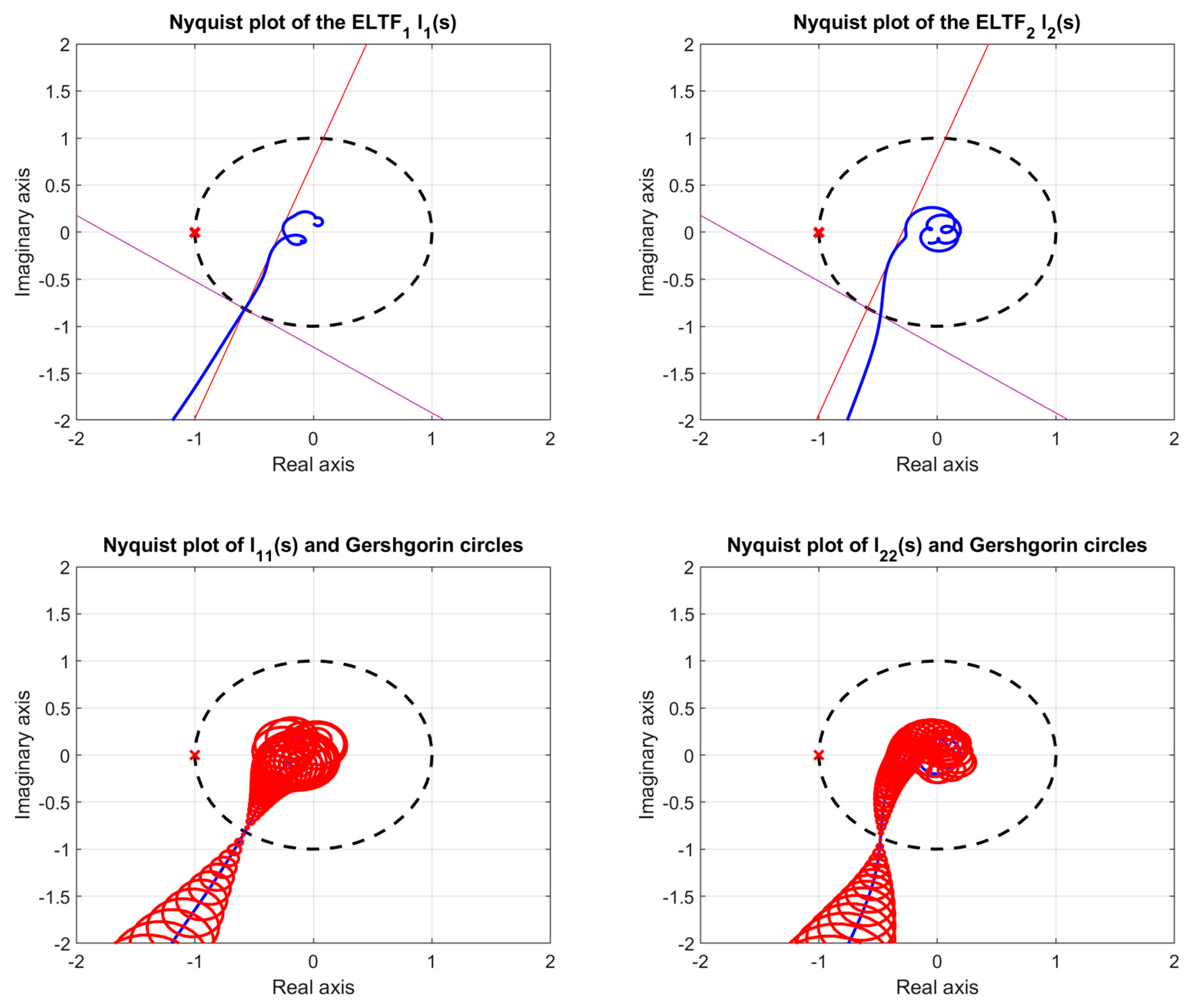
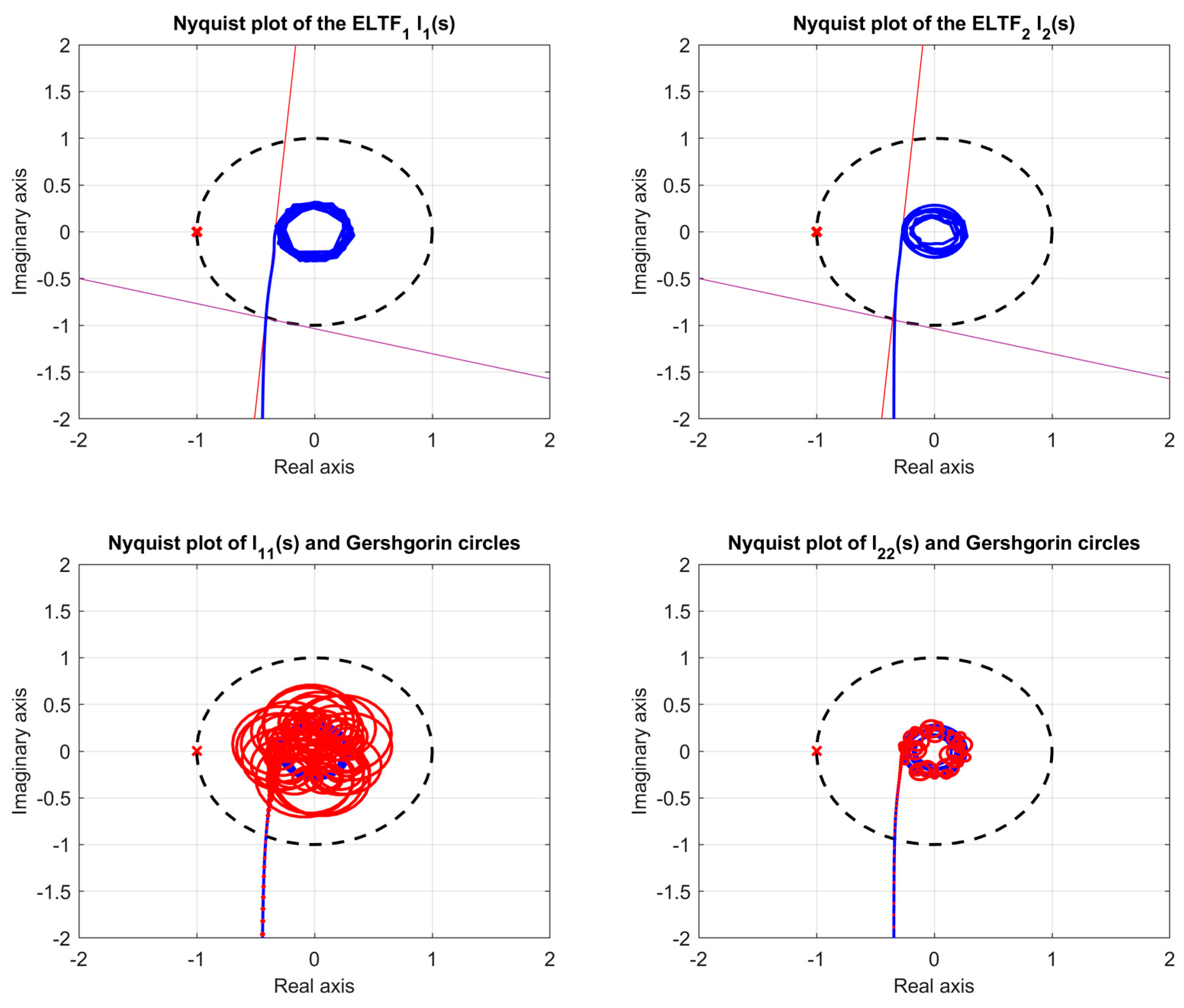
Inequation to prevent the Nyquist polar trace of the diagonal elements of the open-loop matrix L(s) from encircling the critical point. Thus, the ELTFs are stable if the elements of G(s) are stable;

(c)

Equality to achieve static decoupling. As an example, the expressions for the 2 × 2 case in (18) are parameterized with respect to ρ. Here, 0_1×3 represents a row vector of three zero elements;

(d)

Equality to achieve decoupling at the selected ω_x frequencies. The constraint in (19) is linearly parameterized with respect to ρ;

(e)

Lower (LB) and upper (UB) bounds on the design parameters. Integral gains are forced to be positive, whereas proportional and derivative gains can have any sign.

$$\begin{array}{l}\mathrm{maximize}\hspace{1em}\left[0,1,0,0,1,0,0,1,0,0,1,0\right]\mathsf{\rho }\\ \mathrm{subject} \mathrm{to}:\hspace{1em}\\ (a)\{\begin{array}{l}\left[\cot {\alpha }_i\Im \left({\Psi }_{ia}(j{\mathsf{\omega }}_k)\right)-\Re \left({\Psi }_{ia}(j{\mathsf{\omega }}_k)\right)\right]\mathsf{\rho }\le 1-L_{mi}\hspace{1em} \forall {\mathsf{\omega }}_k,\forall i\\ \left[\cot {\alpha }_i\Im \left({\Psi }_{ib}(j{\mathsf{\omega }}_k)\right)-\Re \left({\Psi }_{ib}(j{\mathsf{\omega }}_k)\right)\right]\mathsf{\rho }\le 1-L_{mi}\hspace{1em} \forall {\mathsf{\omega }}_k,\forall i \end{array}\\ (b) \left[\cot {\alpha }_i\Im \left({\Lambda }_{ii}(j{\mathsf{\omega }}_k)\right)-\Re \left({\Lambda }_{ii}(j{\mathsf{\omega }}_k)\right)\right]\mathsf{\rho }\le 0.8\hspace{1em} \forall {\mathsf{\omega }}_k,\forall i\\ (c)\{\begin{array}{c}\left[\begin{array}{cccc}\begin{array}{ccc}{0}_{1\times 3}& 0& sign(k_{12})g_{11}(0)\end{array}& 0& 0_{1\times 3}& \begin{array}{ccc}0& sign(k_{22})g_{12}(0)& 0\end{array}\end{array}\right]\mathsf{\rho }=0\\ \left[\begin{array}{cccc}\begin{array}{ccc}0& sign(k_{11})g_{21}(0)& 0\end{array}& 0_{1\times 3}& \begin{array}{ccc}0& sign(k_{21})g_{22}(0)& 0\end{array}& 0_{1\times 3}\end{array}\right]\mathsf{\rho }=0\end{array}\\ (d) {\Lambda }_{ij}(j{\mathsf{\omega }}_{xj})\mathsf{\rho }=0\hspace{1em}\forall j,\forall i\ne j\\ (e) LB\le \mathsf{\rho }\le UB\end{array}$$

(20)

3.2.2. Optimization II

The second proposed optimization attempts to maximize the linear robustness margin L_m of each loop with the ELTFs subject to minimum bandwidth requirements, which is related to the crossing frequency ω_c of the phase margin, i.e., the frequency at which the Nyquist plot crosses the unit circle. The higher the crossover frequency, the shorter the rise time and the faster the disturbance rejection.

The conditions defined in (6) are used to define the bandwidth requirements; in them, the frequency ω_x is a lower approximation of the crossover frequency ω_c. The user must specify the angle β defining the line q in Figure 3 and the desired frequency ω_x. This frequency cannot be too high; otherwise, linear programming will not find a solution. For example, in systems with a time delay, ω_x must be less than 5/t_d, t_d being the longest time delay associated with the ELTF. Substituting (15) in (6), such constraints for the ELTF of loop i can be expressed as a line parameterization of the PID parameter vector ρ as follows in (21) for the ELTF represented with option a. This indicates that the Nyquist plot of the ELTF must lie below the line q at frequencies below ω_x and above it for higher frequencies.

$$\begin{array}{l}\left[\cos {\beta }_i\Im \left({\Psi }_{ia}(j{\mathsf{\omega }}_k)\right)+\sin {\beta }_i\Re \left({\Psi }_{ia}(j{\mathsf{\omega }}_k)\right)\right]\mathsf{\rho }\le -1\hspace{1em} \forall {\mathsf{\omega }}_k\le {\mathsf{\omega }}_{xi}\\ \left[\cos {\beta }_i\Im \left({\Psi }_{ia}(j{\mathsf{\omega }}_k)\right)+\sin {\beta }_i\Re \left({\Psi }_{ia}(j{\mathsf{\omega }}_k)\right)\right]\mathsf{\rho }>-1\hspace{1em} \forall {\mathsf{\omega }}_k>{\mathsf{\omega }}_{xi}\end{array}$$

(21)

Furthermore, in this optimization, it must be considered that the distances L_m of the linear margins of robustness to be maximized in each loop must be added as a variable to the vector of decision variables. Thus, as an example, for the 2 × 2 case, the new design vector θ would be defined as shown in (22): first, the vector of the PID parameters ρ and then the two linear margins are symbolized by ℓ₁ and ℓ₂. On the latter, a lower bound of 0.3 and a maximum of 0.95 are imposed.

$$\mathsf{\theta }={\left(\begin{array}{ccc}{\mathsf{\rho }}^T& {\mathsf{\ell }}_1& {\mathsf{\ell }}_2\end{array}\right)}^T$$

(22)

In the case of 2 × 2 processes, the linear programming method defining the proposed optimization II is shown in (23), where the objective function and constraints are parameterized with respect to the new vector of the decision variables θ in (22). The objective function maximizes ℓ₁ and ℓ₂, which are the only variables multiplied by 1. Some constraints in (23) are similar to those in optimization problem I, but others change, are sometimes not advised, or are new. These constraints are as follows:

(a)

Inequations to meet the bandwidth specification ω_x in each ELTF. To improve the convergence of the iterative method, the two proposed expressions of the ELTFs are used: one that only depends on the associated column controllers (option a) and one that depends on all the control elements (option b);

(b)

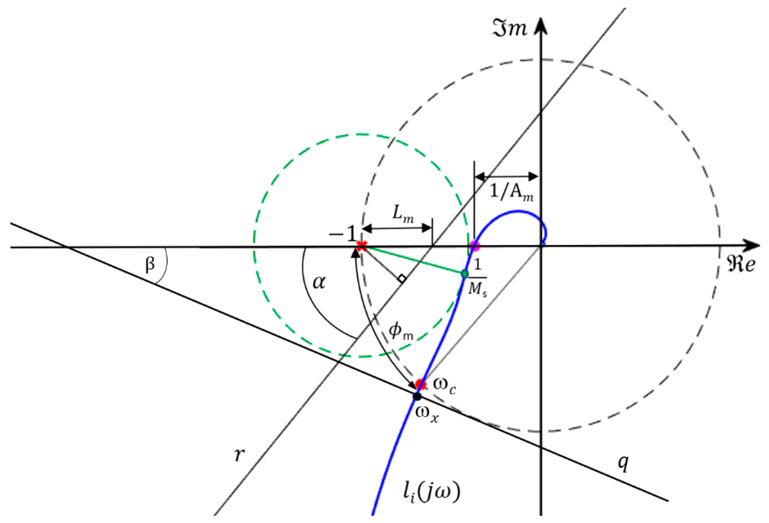
Inequation for the fulfillment of the linear margin by each ELTF similar to optimization I but with two differences: the linear margin is now a decision variable; and, in addition, this constraint is now only required for frequencies higher than ω_x. For lower frequencies, it is not required to be to the right of line r in Figure 3 since the previous constraint renders the Nyquist plot of the ELTF to be below the line q defined by β and tangent to the unit circle for frequencies below ω_x. This constraint also causes the polar trace to move away from the critical point −1;

(c)

Inequation to prevent the polar trace of the diagonal elements of the open-loop matrix L(s) from encircling the critical point. It is similar to optimization I but is parameterized with respect to θ;

(d)

Equality to achieve static decoupling. This is similar to optimization I but is parameterized with respect to θ;

(e)

Equality to achieve decoupling at frequency ω_x. This is similar to optimization I but is parameterized with respect to θ. However, it must be said that in optimization II, adding this may reduce the achievable bandwidth;

(f)

Lower (LB) and upper (UB) bounds on the design parameters.

$$\begin{array}{l}\mathrm{maximize}\hspace{1em}\left[\begin{array}{ccc}{0}_{1x12}& 1& 1\end{array}\right]\mathsf{\theta }\\ \mathrm{subject} \mathrm{to}:\hspace{1em}\\ (a)\{\begin{array}{l}\left[\begin{array}{ccc}\cos {\mathsf{\beta }}_i·\Im \left({\Psi }_{iz}(j{\mathsf{\omega }}_k)\right)+\sin {\mathsf{\beta }}_i·\Re \left({\Psi }_{iz}(j{\mathsf{\omega }}_k)\right)& 0& 0\end{array}\right]\mathsf{\theta }\le -1\hspace{1em} \forall {\mathsf{\omega }}_k\le {\mathsf{\omega }}_{xi},\forall i,\forall z=a,b\\ \left[\begin{array}{ccc}\cos {\mathsf{\beta }}_i·\Im \left({\Psi }_{iz}(j{\mathsf{\omega }}_k)\right)+\sin {\mathsf{\beta }}_i·\Re \left({\Psi }_{iz}(j{\mathsf{\omega }}_k)\right)& 0& 0\end{array}\right]\mathsf{\theta }>-1\hspace{1em} \forall {\mathsf{\omega }}_k>{\mathsf{\omega }}_{xi},\forall i,\forall z=a,b\end{array}\\ (b)\{\begin{array}{l}\left[\begin{array}{ccc}\cot {\mathsf{\alpha }}_1·\Im \left({\Psi }_{1z}(j{\mathsf{\omega }}_k)\right)-\Re \left({\Psi }_{iz}(j{\mathsf{\omega }}_k)\right)& 1& 0\end{array}\right]\mathsf{\theta }\le 1\hspace{1em} \forall {\mathsf{\omega }}_k>{\mathsf{\omega }}_{x1},\forall z=a,b\\ \left[\begin{array}{ccc}\cot {\mathsf{\alpha }}_2·\Im \left({\Psi }_{2z}(j{\mathsf{\omega }}_k)\right)-\Re \left({\Psi }_{2z}(j{\mathsf{\omega }}_k)\right)& 0& 1\end{array}\right]\mathsf{\theta }\le 1\hspace{1em}\forall {\mathsf{\omega }}_k>{\mathsf{\omega }}_{x2},\forall z=a,b\end{array}\\ (c) \left[\begin{array}{ccc}\cot {\mathsf{\alpha }}_i·\Im \left({\Lambda }_{ii}(j{\mathsf{\omega }}_k)\right)-\Re \left({\Lambda }_{ii}(j{\mathsf{\omega }}_k)\right)& 0& 0\end{array}\right]\mathsf{\theta }\le 0.8\hspace{1em} \forall {\mathsf{\omega }}_k,\forall i\\ (d)\{\begin{array}{c}\left[\begin{array}{cccc}\begin{array}{ccc}{0}_{1\times 3}& 0& sign(k_{12})·g_{11}(0)\end{array}& 0& 0_{1\times 3}& \begin{array}{ccc}0& sign(k_{22})·g_{12}(0)& \begin{array}{ccc}0& 0& 0\end{array}\end{array}\end{array}\right]\mathsf{\theta }=0\\ \left[\begin{array}{cccc}\begin{array}{ccc}0& sign(k_{11})·g_{21}(0)& 0\end{array}& 0_{1\times 3}& \begin{array}{ccc}0& sign(k_{21})·g_{22}(0)& 0\end{array}& \begin{array}{ccc}{0}_{1\times 3}& 0& 0\end{array}\end{array}\right]\mathsf{\theta }=0\end{array}\\ (e) \left[\begin{array}{ccc}{\Lambda }_{ij}(j{\mathsf{\omega }}_{xj})& 0& 0\end{array}\right]\mathsf{\theta }=0\hspace{1em}\forall j,\forall i\ne j\\ (f) LB\le \mathsf{\theta }\le UB\end{array}$$

(23)

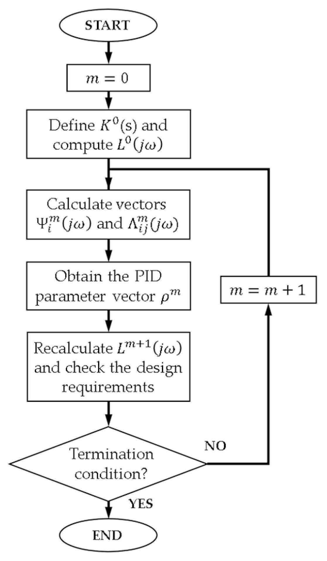
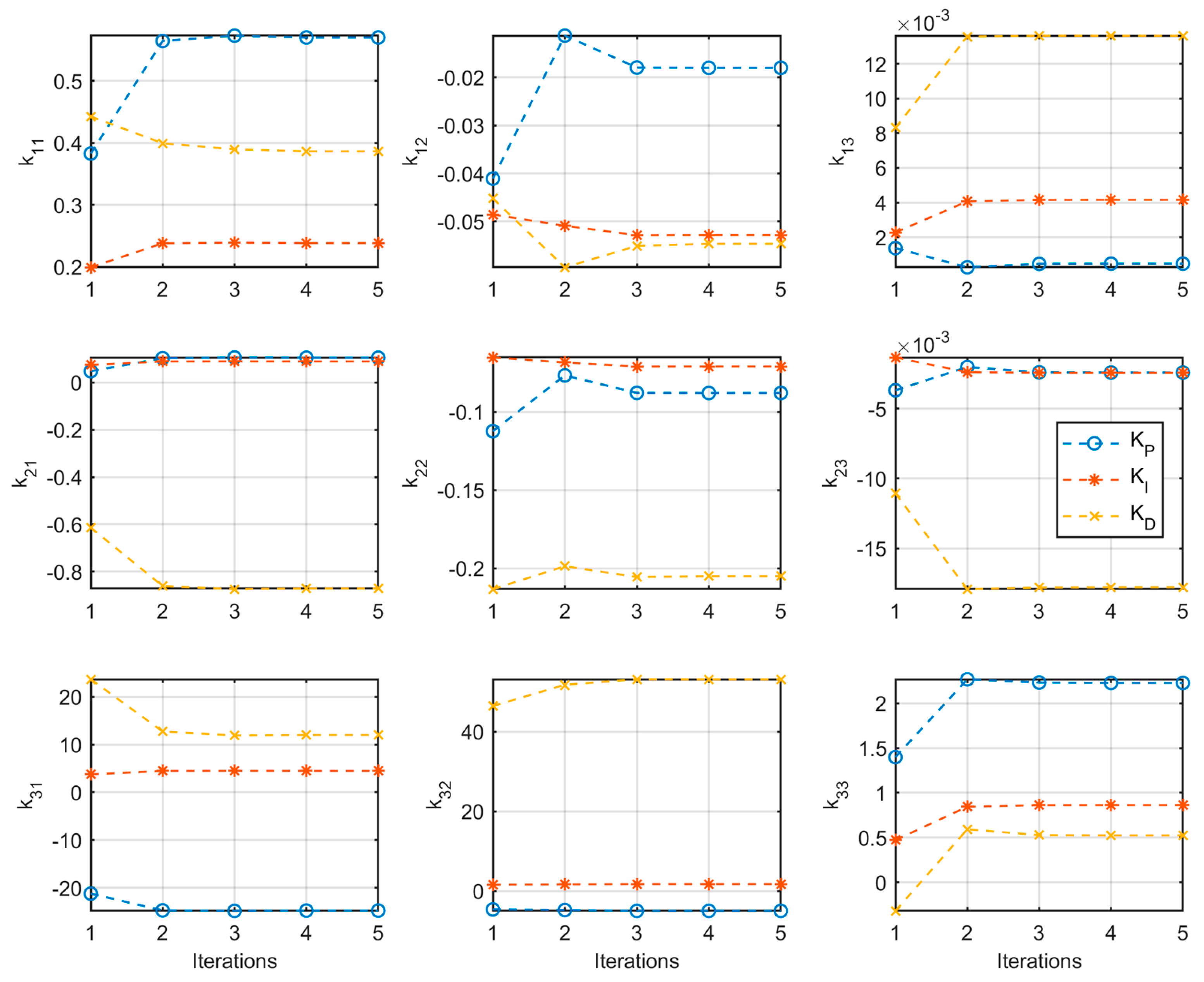
3.3. Iterative Algorithm

The optimizations proposed in the previous section are jointly performed for the ELTFs of the multivariable system to calculate the total PID parameter vector ρ. Because in some constraints some open-loop functions l_ij(s) are assumed to be known, an initial control matrix is required to calculate the open-loop matrix L(s). When the new control matrix K(s) is obtained after optimization, it is necessary to recalculate the matrix L(s), since it will have changed and recheck whether the design specifications are met. If not, iteration is necessary. Therefore, the proposed design method is iterative, and the input data are the process transfer matrix G(s), the design specifications, and an initial control matrix K⁰(s). As the output, it provides the resultant multivariable PID control.

Figure 4 shows the flowchart of the proposed iterative algorithm. First, the iteration variable m is set to 0. Next, an initial control matrix K⁰(s) is chosen, and the frequency response of the open-loop matrix L⁰(jω) is calculated before entering the iterative loop. Although the initial K⁰(s) matrix may somewhat affect the number of iterations, in the analyzed examples, practically the same final controls were obtained using different guesses. Here, we propose to use the inverse of the static gain matrix of the process, which is G(0), because of its computational simplicity and good convergence speed. In the case of non-square processes, the pseudoinverse of G(0) can be used. Then, we enter an iterative loop in which in each iteration m, the following steps are performed:

• Calculate, according to Section 3.1, the vectors Ψ_ia(jω_k), Ψ_ib(jω_k) for the ELTF of each loop and the vectors Λ_ij(jω_k) from the frequency response of the open-loop matrix known from the previous iteration L^m−1(jω);
• Obtain the PID parameter vector ρ^m using the linear programming method proposed in Section 3.2 depending on the design specifications;
• Recalculate the new open-loop matrix frequency response L^m(jω) with the new PID MIMO control matrix. With these open-loop transfer functions, we calculate the new ELTFs and check if the design requirements are met in all the loops;
• If the termination condition is fulfilled, the design is accepted and the resulting vector ρ is used to generate the multivariable PID control matrix K(s); otherwise, the iteration variable m is incremented and the process iterates again. The termination condition is satisfied if, during three consecutive iterations, the variation of the decision variables is below a user-defined tolerance. A maximum number of iterations before the process stops in the case of no convergence is also defined.

Figure 4. Flow chart of the proposed iterative procedure.

Figure 4. Flow chart of the proposed iterative procedure.

After calculating the control parameter vector ρ, the PID elements of the control matrix K(s) are implemented. When implementing the designed PID controllers, the PID structure provided in (24) is used, where u(s) is the control signal, y(s) is the controlled variable, and e(s) is the error signal. This PID structure avoids excessive spikes in the control signal caused by derivative action when there are sudden changes in the reference signal [41]. Derivative action is filtered with a first-order term to render the controllers realizable. A value of N = 20 is chosen so that the effect of the filter can be neglected in the frequency range of interest.

$$u(s)=\left(K_P+\frac{K_I}{s}\right)e(s)-\frac{K_{D}s}{\frac{\left(K_D/K_P\right)}{N}s+1}y(s)$$

(24)

4. Illustrative Examples

In this section, the effectiveness of the proposed methodology is verified in a simulation by applying it to three stable processes of different dimensions: a 2 × 2 square system, a 3 × 3 square system, and a 2 × 3 non-square system. In each example, the proposed multivariable PID control is compared with those proposed by other authors.

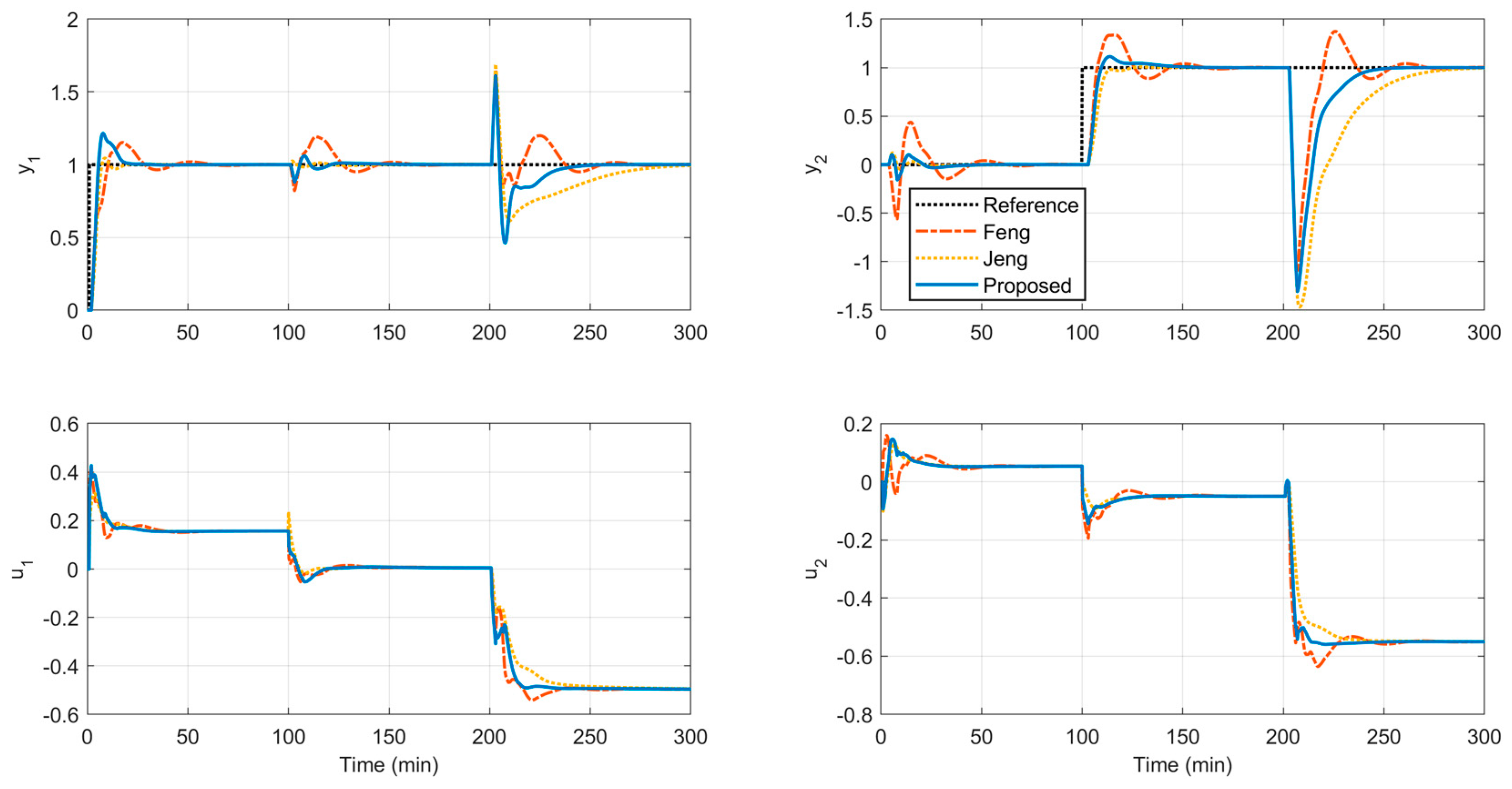
4.1. Example 1: A Wood and Berry Distillation Column

This example uses the distillation column process that is defined by the 2 × 2 transfer matrix G_WB(s) in (25) [42]. It is a classical testbench in multivariate systems because it presents significant interactions and contains multiple time delays. The time constants are expressed in minutes. From G_WB(s), a frequency response array of 1000 elements logarithmically spaced in the frequency range of [10⁻⁵, 5] rad/min is computed. To design the multivariable PID control, optimization II is used with bandwidth design specifications of 0.4 and 0.18 rad/min for loops 1 and 2, respectively. These values were chosen to obtain a response speed similar to that of other authors. In addition, values of α = 70° and β = 35° are specified for both loops, and the two decoupling constraints (d and e) shown in (23) are used.

$$G_{WB}(s)=\left(\begin{array}{cc}\frac{12.8}{16.7s+1}{e}^{-s}& \frac{-18.9}{21s+1}{e}^{-3s}\\ \frac{6.6}{10.9s+1}{e}^{-7s}& \frac{-19.4}{14.2s+1}{e}^{-3s}\end{array}\right)$$

(25)

By using the inverse of G_WB(0) as the initial controller, the proposed method obtains the multivariable PID control shown in (26) in only five iterations, as shown in Figure 5. This figure shows the progression of the PID parameters of each controller k_ij(s) and the margins L_m during the iterative procedure. Considering that the proposed procedure always involves at least three iterations to ensure convergence, in this example, the convergence is quickly achieved. This is partly due to the use of all the proposed constraints for optimization II described in Section 3.2.2. The linear margin values achieved are ℓ₁ = 0.721 and ℓ₂ = 0.704.

$$K_{PID}(s)=\left(\begin{array}{cc}0.3024+\frac{0.1237}{s}+0.2323s& -0.0561-\frac{0.0383}{s}-0.1153s\\ -0.09311+\frac{0.0421}{s}-0.0781s& -0.1086-\frac{0.02597}{s}-0.09423s\end{array}\right)$$

(26)

In the top part of Figure 6, the resulting Nyquist plots for the two ELTFs are shown along with the r and q lines associated with the design constraints. It should be recalled that, in optimization II, the linear margin constraint only applies at frequencies above ω_x.

Table 1. Robustness and performance indices in example 1.

Method	Loop	ϕm	Am	Ms	ωcp (rad/min)	IAE	TV
Proposed	1	54.67	3.99	1.48	0.403	11.88	1.83
	2	61.36	3.75	1.51	0.181	34.82	1.51
Feng	1	76.47	3.36	1.69	0.23	15.67	2.11
	2	45.21	2.22	1.95	0.21	39.96	2.06
Jeng	1	63.5	3.86	1.57	0.31	17.74	1.39
	2	66.4	2.71	1.65	0.13	56.33	1.16

lists the other classical robustness margins and crossover frequency ω_c achieved with the proposed design with those obtained by other authors. Specifically, these other controllers are the centralized PID control designed via an iterative LMI approach by Feng et al. [43] and the centralized PID control for decoupling designed by Jeng et al. via a data-based method in [21]. The proposed control achieves the highest gain margins A_m, the best sensitivity margins M_s, and the highest bandwidth in loop 1. The M_s index is calculated for the corresponding ELTF according to the expression provided in (27).

The bottom part of Figure 6 shows the Nyquist plots of the diagonal elements of the resulting L(s) matrix with the corresponding Gershgorin circles. These results show the diagonal dominance of the resulting open-loop process and how perfect decoupling has been practically achieved at the crossover frequency since the circles around ω_c are almost of zero radius.

Figure 7 shows the closed-loop time response of the proposed PID MIMO control compared with the other two above-mentioned designs. The simulations were performed using a unit step change at t = 1 min in the first reference and at t = 100 min in the second reference. In addition, at t = 200 min, there is a load disturbance consisting of a step change of amplitude 0.5 at both process inputs. From the simulation data, the integrated absolute error (IAE) and the control signal total variation (TV) of each loop are calculated in the time domain. The general expressions are shown in (27). These values are used as performance indices of the time response: the first is related to the error and the second is related to the control effort. These values are also illustrated in Table 1.

$$M_{si}=\max \left|\frac{1}{1+l_i(j\mathsf{\omega })}\right|\hspace{1em}IA{E}_i={\displaystyle \int \left|e_i(t)\right|dt}\hspace{1em}T{V}_i={\displaystyle \int \left|\frac{d{u}_i(t)}{dt}\right|}dt$$

(27)

The proposed MIMO PID control shows a settling time similar to Jeng’s control in loop 1 and somewhat higher in loop 2. Feng’s control has the highest settling time in both loops. The proposed control shows excellent decoupling performance, especially compared to Feng’s control. Jeng’s control achieves almost perfect decoupling because its design is based on full dynamic decoupling; however, this means its response to load disturbance is the slowest of them all. The proposed PID control rejects the load disturbances earlier than the others, which causes it to have the lowest IAE values in Table 1. The IAE values in loops 1 and 2 obtained with the proposed control are, respectively, 24.2% and 12.9% lower than Feng’s values and 33% and 38.2% lower than those of Jeng’s control. Moreover, this response is achieved with TV values similar to or lower than those of the other methods. The TV values of the proposed control in loops 1 and 2 are 13.3% and 26.7% lower than Feng’s values, respectively. Compared to Jeng’s control, the proposed control achieves better IAE values at the expense of an increase of approximately 30% in the TV values of both loops.

4.2. Example 2: An Ogunnaike and Ray Distillation Column

The transfer matrix of this process is provided in the 3 × 3 G_OR(s) matrix in (28) [44]. This is a process with multiple time delays and significant interactions, where the time constants are expressed in minutes. From this matrix, a frequency response array of 1000 elements in the range of [10⁻⁵, 5] rad/min is obtained. In this example, optimization I is applied with robustness specifications provided in L_m, with values of 0.85, 0.8, and 0.65, and α values equal to 85°, 80°, and 65° for loops 1, 2, and 3, respectively. In addition, the decoupling constraint d is applied at frequencies 0.16, 0.18, and 0.8 rad/min, respectively, in each loop. After five iterations, the multivariable PID control provided in (29) is obtained. Figure 8 shows the progression of the PID parameters using the inverse of the G_OR(0) matrix as the initial control matrix K⁰. Although this second example has a higher dimension than the previous example, the proposed iterative procedure quickly converges.

$$G_{OR}(s)=\left(\begin{array}{ccc}\frac{0.66}{6.7s+1}{e}^{-2.6s}& \frac{-0.61}{8.64s+1}{e}^{-3.5s}& \frac{-0.0049}{9.06s+1}{e}^{-s}\\ \frac{1.11}{3.25s+1}{e}^{-6.5s}& \frac{-2.36}{5s+1}{e}^{-3s}& \frac{-0.01}{7.09s+1}{e}^{-1.2s}\\ \frac{-34.68}{8.15s+1}{e}^{-9.2s}& \frac{46.2}{10.9s+1}{e}^{-9.4s}& \frac{0.87(11.61s+1)}{(3.89s+1)(18.8s+1)}{e}^{-s}\end{array}\right)$$

(28)

$$K_{PID}(s)=\left(\begin{array}{ccc}0.5689+\frac{0.2384}{s}+0.3863s& -0.01799-\frac{0.05284}{s}-0.05466s& 0.0004698+\frac{0.004157}{s}+0.01363s\\ 0.1051+\frac{0.08933}{s}-0.8716s& -0.08796-\frac{0.07105}{s}-0.205s& -0.00241-\frac{0.00243}{s}-0.01779s\\ -24.75+\frac{4.486}{s}+12s& -4.99+\frac{1.727}{s}+53.11s& 2.227+\frac{0.8624}{s}+0.5243s\end{array}\right)$$

(29)

The top part of Figure 9 shows the Nyquist plots of the three resulting ELTFs, where the fulfillment of the linear margin constraint is verified.

Table 2. Robustness and performance indices in example 2.

Method	Loop	ϕm	Am	Ms	ωcp (rad/min)	IAE	TV
Proposed	1	77.52	6.67	1.18	0.081	13.44	4.16
	2	73.04	5.37	1.26	0.086	22.30	2.55
	3	53.79	3.60	1.48	0.395	107.6	240.3
Silva	1	63.32	4.92	1.42	0.191	12.85	4.38
	2	55.06	7.4	1.67	0.191	32.12	2.61
	3	48.38	3.02	1.69	0.554	112.5	210.0
Ram	1	62.11	4.83	1.33	0.120	10.38	4.85
	2	71.07	2.57	1.64	0.118	23.70	3.87
	3	95.29	11.42	1.25	0.119	634.6	169.2

shows the other classical robustness indices for each loop. For comparison, the indices obtained with the controllers proposed by other authors are also shown. One of these controllers is the decentralized PID control of Silva and Barros [45], which was designed via an iterative method in the frequency domain. The other is the centralized PI control of Ram and Chidambaram [17], which is based on the combination of static decoupling and multiloop PI control. The proposed control achieves very robust margins mainly in the first two loops, where it has the largest phase margins and the lowest maximum sensitivity values; however, it has the lowest cutoff frequencies. Ram’s proposed control has the most robust design for the third loop. The bottom part of Figure 9 shows the Nyquist plots of the diagonal open-loop processes of L(s) with the Gershgorin circles. The small circles in l₁₁(s) and l₂₂(s) indicate good diagonal dominance in these loops, not so in l₃₃(s) with very large circles, which causes this loop to exhibit significant interaction.

Figure 10 shows the closed-loop time responses achieved with the proposed MIMO PID control and the controllers of the two aforementioned authors. In the simulation, there is a unit step change in references 1, 2, and 3 at t = 1 min, t = 100 min, and t = 200 min, respectively. In addition, there is a 0.5 step change in all the process inputs at t = 300 min as a load disturbance. Table 2 lists the corresponding IAE and TV values. In the reference tracking performance in loops 1 and 2, the proposed control has a slightly slower rise time than the other loops, but similar settling time and no overshoot. In loop 3, the proposed control and Ram’s controller are faster than Silva’s control. In terms of disturbance rejection, the three controllers have a similar response. In terms of decoupling performance, the proposed control outperforms the other two, because owing to the two decoupling constraints imposed in the optimization, it has the best decoupling performance. Because of this, the proposed control obtains the lowest IAE values in loops 2 and 3, where the interactions are stronger.

The IAE values in loops 2 and 3 of the proposed control are 30.6% and 4.6% lower than those of Silva, respectively, and 5.9% and 83% lower than those of Ram’s control. However, the IAE value in loop 1 is 4.6% higher than that of Silva and 29.5% higher than that of Ram. The proposed control has the lowest TV values in loops 1 and 2, which are, respectively, 5% and 2.3% lower than those of Silva and 14.2% and 34.1% lower than those of Ram. However, it achieves the highest TV value in loop 3, which is 14.4% higher than that of Silva and 42% higher than that of Ram.

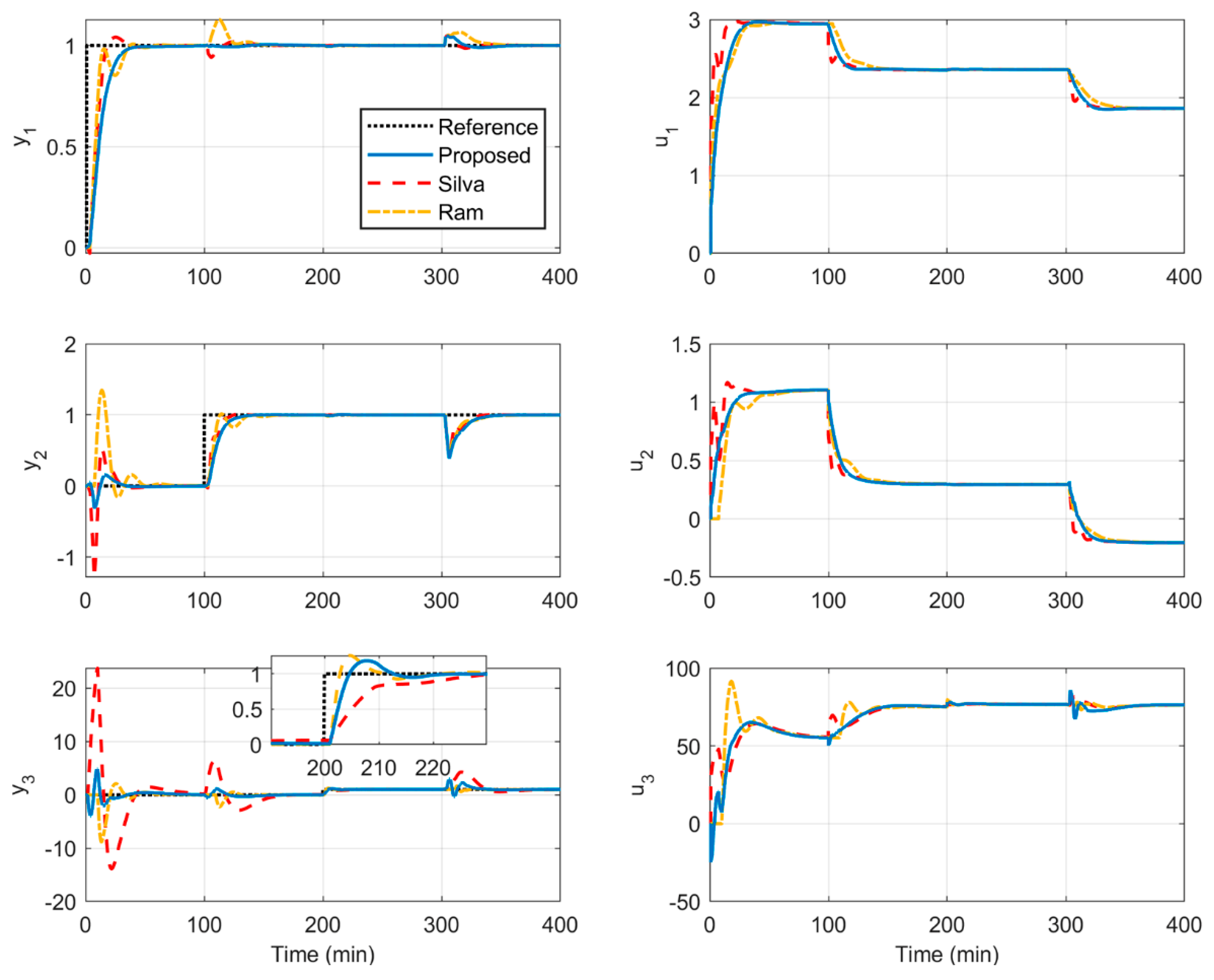
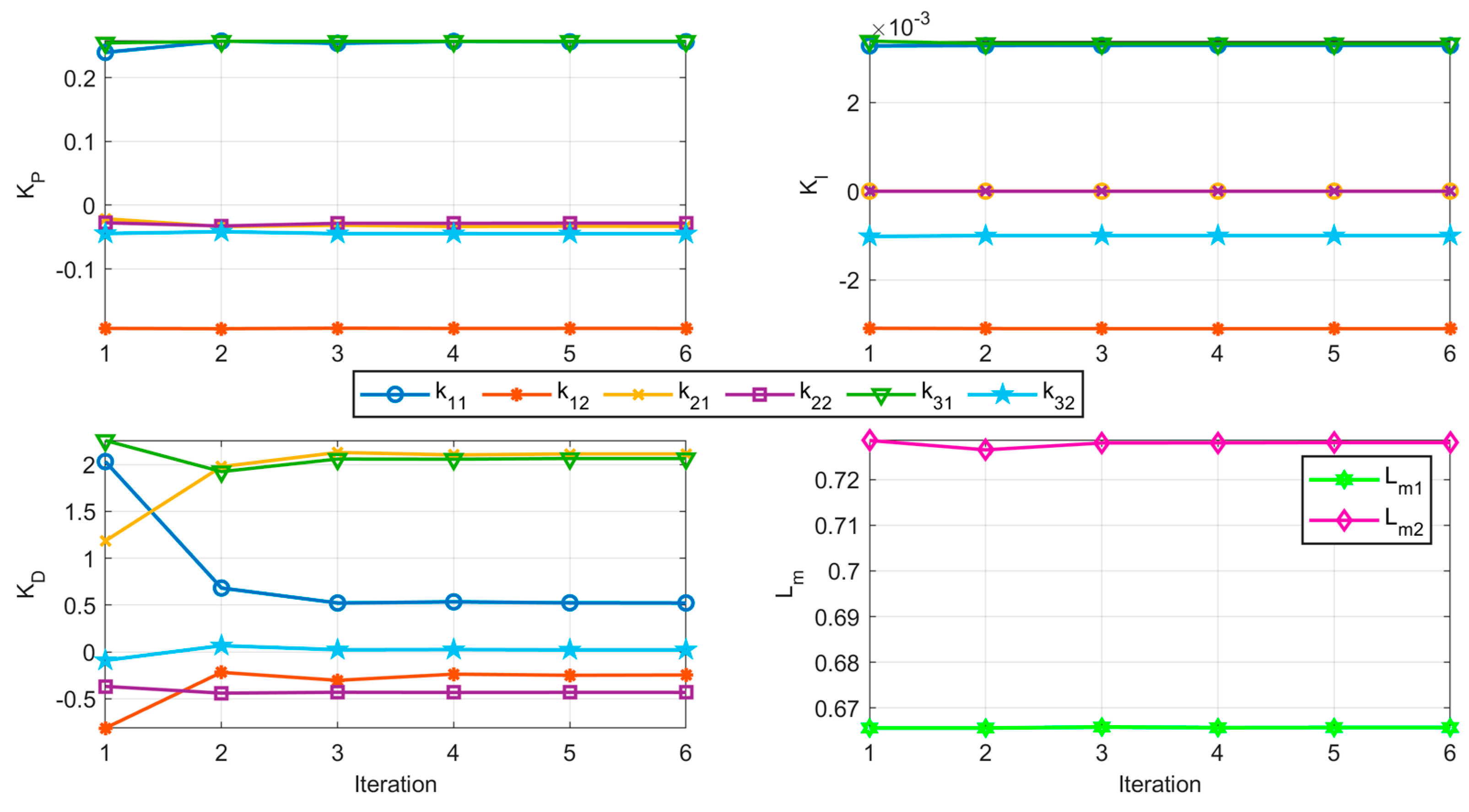
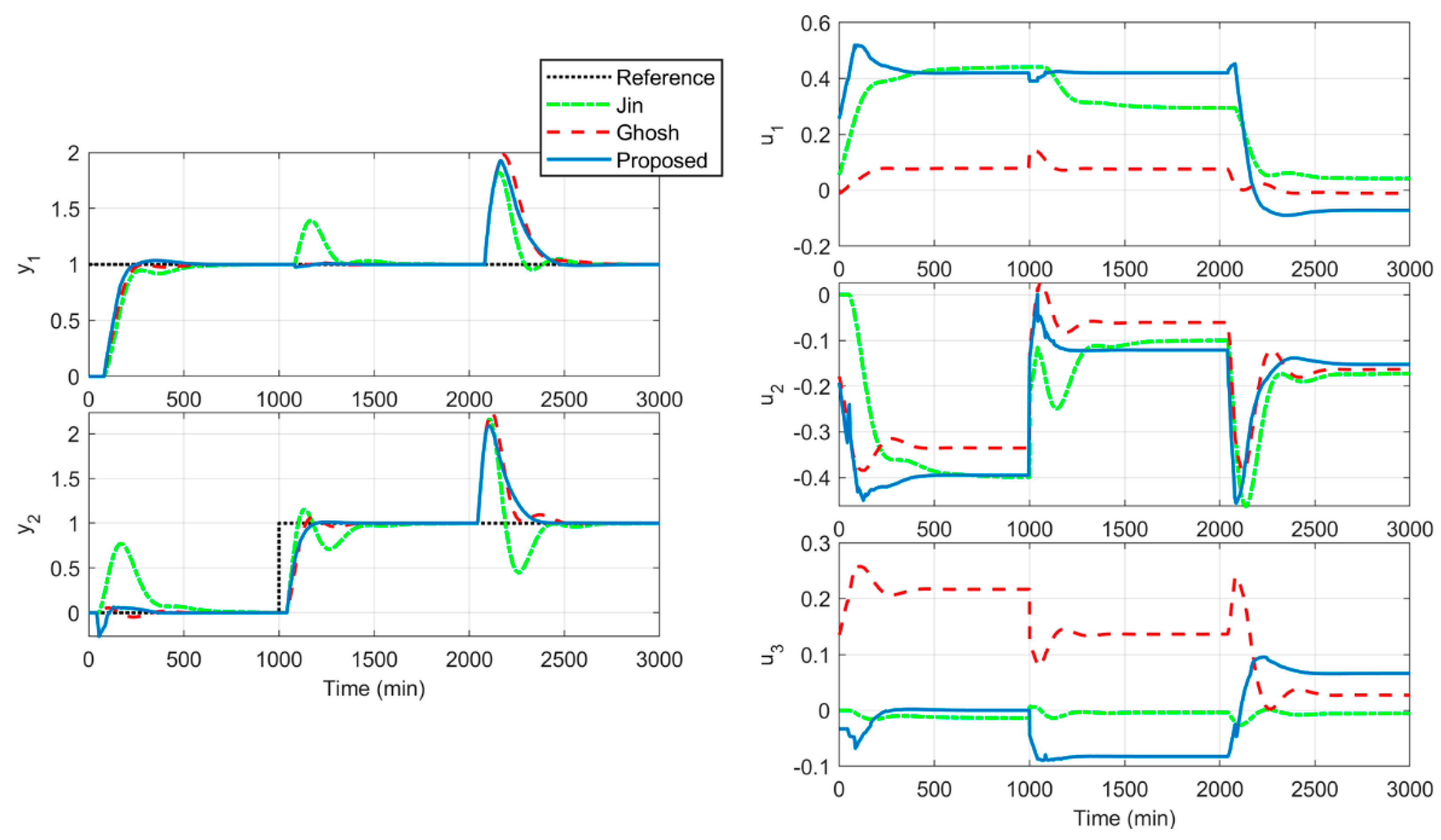
4.3. Example 3: 2 × 3 Shell Process

In this example, the system to be controlled is a non-square subset of the Shell process with two outputs and three inputs representing a heavy oil fractionator [36]. This is provided in the 2 × 3 matrix G_SH(s) in (30). The process, besides being a multivariable non-square system, shows significant interaction and contains significant time delays. The time constants are expressed in minutes. A frequency response array of 1000 elements in the range of [10⁻⁶, 1] rad/min is obtained from this matrix.

To design the multivariable PID control, optimization II is used with bandwidth design specifications of 0.0075 and 0.012 rad/min for loops 1 and 2, respectively, in order to obtain cut-off frequencies similar to those of other authors. In addition, values of α = 85° and β = 15° are specified for both loops, and the two decoupling constraints (d) and (e) shown in (23) are used.

$$G_{SH}(s)=\left(\begin{array}{l}\begin{array}{ccc}\frac{4.05e^{-81s}}{50s+1}& \frac{1.77e^{-84s}}{60s+1}& \frac{5.88e^{-81s}}{50s+1}\end{array}\\ \begin{array}{ccc}\frac{5.39e^{-54s}}{50s+1}& \frac{5.72e^{-42s}}{60s+1}& \frac{6.9e^{-45s}}{40s+1}\end{array}\end{array}\right)$$

(30)

Taking the pseudoinverse of G_SH(0) as the initial control K⁰, the proposed method obtains the 3 × 2 PID control shown in (31) after six iterations, as shown in Figure 11. This figure shows the progress of the PID parameters and margins L_m during the iterative process. The linear margin values achieved are ℓ₁ = 0.666 and ℓ₂ = 0.728.

$$K_{PID}(s)=\left(\begin{array}{cc}\begin{array}{l}0.2564+\frac{0.003289}{s}+0.522s\\ -0.1933-\frac{0.0031}{s}-0.2463s\\ -0.03307+\frac{{10}^{-6}}{s}+2.113s\end{array}& \begin{array}{l}-0.0282-\frac{{10}^{-6}}{s}-0.4319s\\ 0.2571+\frac{0.003325}{s}+2.063s\\ -0.04469-\frac{0.001}{s}+0.0225s\end{array}\end{array}\right)$$

(31)

The Nyquist plots of the two resulting ELTFs with the r and q lines associated with the design constraints are shown at the top of Figure 12.

Table 3. Robustness and performance indices in example 3.

Method	Loop	ϕm	Am	Ms	ωcp (rad/min)	IAE	TV
Proposed	1	65.71	2.99	1.51	0.0077	297.3	1.0841 1.8018 0.4862
	2	70.34	3.55	1.38	0.0121	253.7
Ghosh	1	65.32	2.66	1.67	0.007	328.5	0.3765 1.4852 0.7961
	2	61.02	2.71	1.75	0.0127	264.1
Jin	1	69.79	2.42	1.73	0.006	343	0.8033 1.6588 0.1416
	2	38.81	2.24	2.07	0.0202	451.2

lists the other classical robustness margins and crossover frequency ω_c achieved with the proposed design with those obtained by two other authors. Specifically, the table also shows the values obtained with the centralized PI control of Ghosh and Pan [36], and the multiloop PID controller of Jin et al. [32]. The proposed control achieves similar phase margins, better gain margins, and better maximum sensitivity values. It also achieves the highest bandwidth in loop 1. Figure 12 shows the Nyquist plots of the diagonal elements of the resulting open-loop matrix L(s) with the corresponding Gershgorin circles. The circles with near-zero radii indicate that diagonal dominance is achieved in the system.

The closed-loop time response of the proposed 3 × 2 PID control compared with the other two above-mentioned designs is shown in Figure 13. The simulations were performed using a unit step change in the references at t = 0.1 min in the first reference and at t = 1000 min in the second reference. In addition, at t = 2000 min, there is a load disturbance consisting of a 0.1 step change at the three process inputs. The proposed control and Ghosh’s centralized PI control have a similar response with similar rise times and settling times and excellent decoupling performance; the proposed control is slightly better in disturbance rejection. Jin’s control shows more interaction, which is logical as it is a multiloop PID control. From the simulations, we calculated the IAE and TV values, which are shown in Table 3. In the TV column, there are three values for each design because there are three control signals. The proposed control achieves the lowest IAE values, which are 9.5% and 3.9% lower in loops 1 and 2 than those of Ghosh, respectively, and 13.3% and 43.8 lower than those of Jin. However, it has higher TV values. The TV values obtained with the proposed control in control signals 1 and 2, respectively, are 187% and 21% higher than those of Ghosh; the TV of the third signal is 39% lower than that of Ghosh. Compared with Jin’s control, these TV values are 35%, 8.6%, and 243% higher in control signals 1, 2, and 3, respectively. Because the proposed methodology does not consider the input sensitivity function, the resulting controller can generate large control signals when the closed-loop bandwidth is chosen to be much larger than the open-loop bandwidth [40].

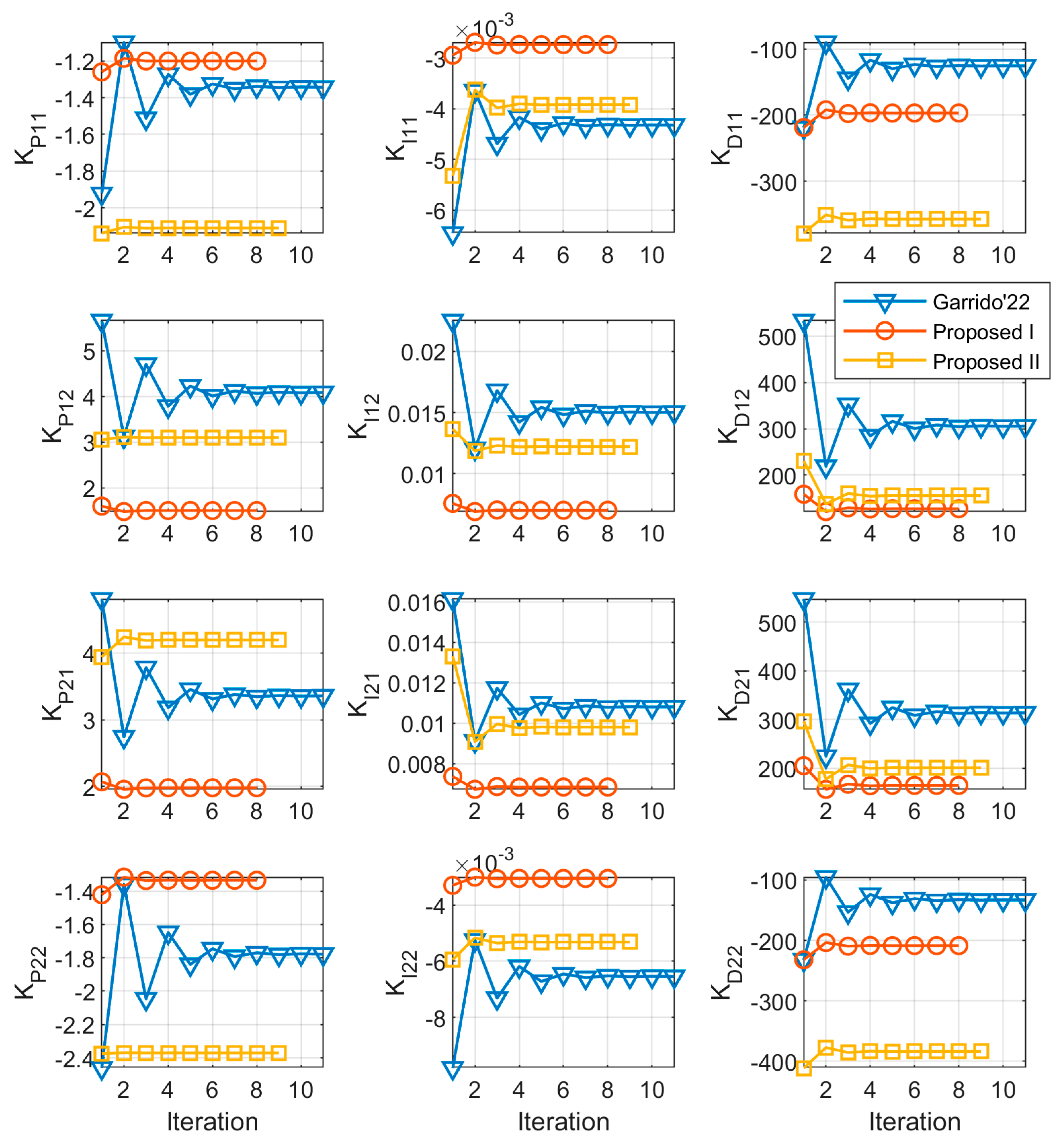
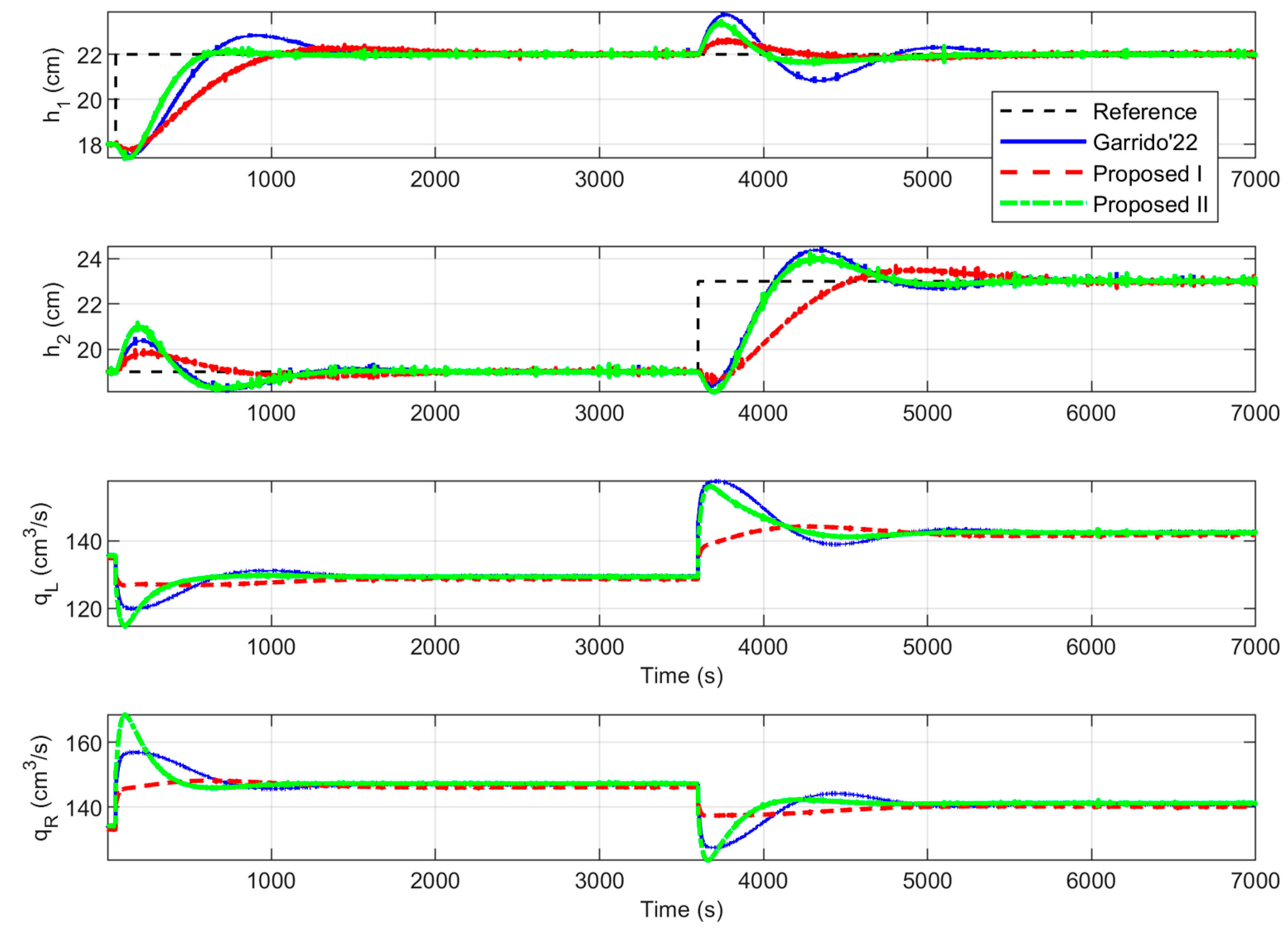
4.4. Example 4: Experimental Quadruple Tank System

In this case, the two proposed methods (I and II) are applied to an experimental process: the quadruple tank plant [46] of the process control lab of the University of Cordoba. It is a 2 × 2 system where the controlled variables are the levels, h₁ and h₂ in cm, of the two lower tanks, and the control signals are the flow references, q_L and q_R in cm³/s, of the secondary loops that command the pumps. The plant is configured to have interaction problems and a multivariable right-half plane (RHP) of zero. The transfer matrix in (32) shows the identified model of the process around the operation point h = [17, 18] cm and q = [135, 135] cm³/s. The time constants are expressed in seconds. The model in (32) has an RGA with diagonal elements equal to −0.21 and a multivariable RHP zero at s = 1/164.7.

$$G_T(s)=\left(\begin{array}{cc}\frac{0.175}{191.5s+1}& \frac{0.402}{(170.5s+1)(260.7s+1)}\\ \frac{0.385}{(165s+1)(240.4s+1)}& \frac{0.154}{178.6s+1}\end{array}\right)$$

(32)

From this matrix, a frequency response array of 1000 elements in the range of [10⁻⁶, 1] rad/s is obtained. To design the multivariable PID control with the proposed optimization I, the robustness specification provided with an L_m value of 0.8 and α value of 75° is used for both loops. In addition to the static decoupling, the decoupling constraint d is applied at a frequency of 0.002 rad/s in each loop. To apply the proposed optimization II, a bandwidth design specification of 0.004 rad/s is used for both loops. In addition, values of α = 75° and β = 35° are specified for both loops, and the two decoupling constraints (d and e) shown in (23) are used. Taking the inverse of G_T(0) as the initial control K⁰, the proposed methods I and II obtain the 2 × 2 PID control shown in (33) and (34), respectively. In the case of optimization II, the linear margin values achieved are ℓ₁ = 0.64 and ℓ₂ = 0.63. For comparison, the previous iterative methodology by Garrido et al. in [39], which is extended in this study, is also applied to this example with a specification provided with L_m = 0.8 and α = 75° in both loops. The resultant MIMO PID control K_G(s) is shown in (35).

$$K_{OPT\_I}(s)=\left(\begin{array}{cc}-1.2-\frac{0.0027}{s}-196.8s& 1.51+\frac{0.007}{s}+127.4s\\ 1.98+\frac{0.0068}{s}+164.9s& -1.33-\frac{0.0031}{s}-208.5s\end{array}\right)$$

(33)

$$K_{OPT\_II}(s)=\left(\begin{array}{cc}-2.11-\frac{0.0039}{s}-357.3s& 3.1+\frac{0.0122}{s}+155.6s\\ 4.19+\frac{0.0098}{s}+201.2s& -2.37-\frac{0.0053}{s}-383.7s\end{array}\right)$$

(34)

$$K_G(s)=\left(\begin{array}{cc}-1.34-\frac{0.0043}{s}-125.6s& 4.09+\frac{0.015}{s}+305.8s\\ 3.36+\frac{0.011}{s}+313.9s& -1.78-\frac{0.0065}{s}-133.1s\end{array}\right)$$

(35)

Figure 14 shows the progress of the PID parameters during the iterative process in the three methodologies. The fact of performing the design of all the PID control parameters of K(s) in each iteration and the new decoupling constraints help the convergence of the proposed methods. The methods performed with optimization I (proposed I) and optimization II (proposed II) require eight and nine iterations, respectively, whereas Garrido’s previous method converges in eleven iterations.

Table 4. Robustness and performance indices in example 4.

Method	loop	ϕm	Am	Ms	ωcp (rad/s)	IAE	TV
Proposed I	1	65.7	5	1.26	2.1 × 10−3	2674.1	464.6
	2	66.4	5	1.26	2.1 × 10−3	3117.4	446.8
Proposed II	1	60.9	2.75	1.59	4 × 10−3	1950.8	699.3
	2	56	2.72	1.58	4 × 10−3	2814.0	652.9
Garrido	1	64.7	5	1.26	3 × 10−3	3233.8	705.3
	2	64.4	5	1.25	4 × 10−3	2931.5	660.8

lists the classical robustness margins and crossover frequencies ω_c achieved with the three designs. Proposed I and Garrido’s design obtain almost the same values of these margins because both are very similar and aim to maximize the integral gains while fulfilling the same robustness margin specification. However, the proposed I design shows lower bandwidth frequencies than Garrido’s; this is a consequence of achieving better diagonal dominance and better decoupling performance imposed by the new decoupling constraints in optimization I. The proposed II design is performed by specifying a higher bandwidth frequency than that obtained with optimization I. As a result, the proposed II control obtains the highest bandwidth frequencies but achieves lower robustness margins than the other two designs.

The closed-loop time responses of the multivariable PID designs are shown in Figure 15. The experiments were performed using a 4 cm step change at t = 50 s in the first reference and at t = 3600 s in the second reference. The inverse response to the step change in the references is due to multivariable RHP zero. The proposed I design has the slowest rise times but the best decoupling performance. The proposed II design shows the fastest response in both loops. Garrido’s control shows a very similar response in loop 2 as the proposed II design; however, in loop 1, it has a slower response than the proposed II design and shows more interaction than the other two designs.

The IAE and TV values calculated from the experimental data are listed in Table 4. The proposed II control presents the lowest IAE values, which are 27% and 9.7% lower than those of the proposed I design in loops 1 and 2, respectively, and 39.7% and 4% lower than those of Garrido’s design. On the other hand, the proposed I design has the lowest TV values, which are approximately 32–34% lower than those of the proposed II control and those of the Garrido’22 design.

5. Conclusions

This paper proposes a new iterative method for centralized PID control design that can be applied to stable processes. The methodology is based on the loop shaping of the Nyquist plot of the equivalent loop transfer function (ELTF) in centralized control, which captures the dynamics and interactions with the other loops. By working with arrays of the frequency response, the method does not require approximations, even when the process has time delays or irrational functions. The method is an extension of our previous methodology in [39]. Its main improvements are the following:

• The complete design of the entire control matrix is formulated at each iteration as a single linear programming problem in which the frequency response of the ELTFs and the open-loop transfer functions are linearly parameterized with respect to the PID parameter vector. In this way, a better convergence is sought. In our previous work, each column of the controller matrix was separately designed;
• Two constraints are proposed to improve the decoupling performance: static decoupling at ω = 0 and decoupling at a frequency close to the crossover frequency of the ELTFs. These constraints not only manage to considerably reduce the interactions but also help to improve the convergence of the iterative procedure;
• Two possible optimizations are proposed according to the design specifications: (I) maximize the integral gains to optimize the disturbance rejection response while complying with a minimum linear robustness margin in each loop and (II) maximize the linear robustness margins of each loop while ensuring minimum bandwidth in each loop. In our previous work, the only option was optimization I;
• The new methodology has been extended not only for square processes but also for non-square systems.

The effectiveness of the proposed method is demonstrated in simulations on three processes of 2 × 2, 3 × 3, and 2 × 3 dimensions as well as a real quadruple tank system. Comparison with other authors’ designs indicated that the proposed methodology achieves similar or superior performance. The main limitations of the methodology are as follows: (a) convergence is not completely assured because the design specifications may not be achievable; (b) the method is restricted to stable processes because the linear margin is not valid for unstable systems; and (c) the magnitude of the control signals is not considered in the optimization, so the designed control may produce high control signals when the bandwidth in the closed-loop is too high.

References

1. Martínez-Luzuriaga, P.N.; Reynoso-Meza, G. Influencia de Los Hiper-Parámetros En Algoritmos Basados En Evolución Diferencial Para El Ajuste de Controladores del tipo PID en Procesos SISO. Rev. Iberoam. De Automática E Informática Ind. 2023, 20, 44–55. [Google Scholar] [CrossRef]
2. De Aguiar, A.P.V.A.; Acioli, G.; Barros, P.R. Frequency-Based Multivariable Control Design with Stability Margin Constraints: A Linear Matrix Inequality Approach. J. Process Control 2023, 132, 103115. [Google Scholar] [CrossRef]
3. Rojas, J.D.; Arrieta, O.; Vilanova, R. Industrial PID Controller Tuning with a Multiobjective Framework Using MATLAB®, 1st ed.; Springer: Cham, Swizterland, 2022; ISBN 978-3-030-72313-2. [Google Scholar]
4. Hägglund, T. The One-Third Rule for PI Controller Tuning. Comput. Chem. Eng. 2019, 127, 25–30. [Google Scholar] [CrossRef]
5. Garrido, J.; Vázquez, F.; Morilla, F. Multivariable PID Control by Decoupling. Int. J. Syst. Sci. 2016, 47, 1054–1072. [Google Scholar] [CrossRef]
6. Jeng, J.C.; Lee, M.W. Multi-Loop PID Controllers Design with Reduced Loop Interactions Based on a Frequency-Domain Direct Synthesis Method. J. Frankl. Inst. 2023, 360, 2476–2506. [Google Scholar] [CrossRef]
7. Mahapatro, S.R.; Subudhi, B. A New Hinf Weighted Sensitive Function Based Robust Multi-Loop PID Controller for a Multi-Variable System. IEEE Trans. Circuits Syst. II Express Briefs, 2023; early access. [Google Scholar] [CrossRef]
8. Hovd, M.; Skogestad, S. Sequential Design of Decentralized Controllers. Automatica 1994, 30, 1601–1607. [Google Scholar] [CrossRef]
9. Mahapatro, S.R.; Subudhi, B. A Robust Decentralized PID Controller Based on Complementary Sensitivity Function for a Multivariable System. IEEE Trans. Circuits Syst. II Express Briefs 2020, 67, 2024–2028. [Google Scholar] [CrossRef]
10. Euzebio, T.A.M.; Da Silva, M.T.; Yamashita, A.S. Decentralized PID Controller Tuning Based on Nonlinear Optimization to Minimize the Disturbance Effects in Coupled Loops. IEEE Access 2021, 9, 156857–156867. [Google Scholar] [CrossRef]
11. Euzébio, T.A.M.; Yamashita, A.S.; Pinto, T.V.B.; Barros, P.R. SISO Approaches for Linear Programming Based Methods for Tuning Decentralized PID Controllers. J. Process Control 2020, 94, 75–96. [Google Scholar] [CrossRef]
12. Garrido, J.; Ruz, M.L.; Morilla, F.; Vázquez, F. Iterative Method for Tuning Multiloop Pid Controllers Based on Single Loop Robustness Specifications in the Frequency Domain. Processes 2021, 9, 140. [Google Scholar] [CrossRef]
13. Arrieta, O.; Vilanova, R. Simple Servo/Regulation Proportional-Integral-Derivative (PID) Tuning Rules for Arbitrary M s-Based Robustness Achievement. Ind. Eng. Chem. Res. 2012, 51, 2666–2674. [Google Scholar] [CrossRef]
14. Vilanova, R.; Arrieta, O.; Ponsa, P. Robust PI/PID Controllers for Load Disturbance Based on Direct Synthesis. ISA Trans. 2018, 81, 177–196. [Google Scholar] [CrossRef]
15. Liu, L.; Tian, S.; Xue, D.; Zhang, T.; Chen, Y.Q.; Zhang, S. A Review of Industrial MIMO Decoupling Control. Int. J. Control Autom. Syst. 2019, 17, 1246–1254. [Google Scholar] [CrossRef]
16. Garrido, J.; Vázquez, F.; Morilla, F. Centralized Multivariable Control by Simplified Decoupling. J. Process Control 2012, 22, 1044–1062. [Google Scholar] [CrossRef]
17. Dhanya Ram, V.; Chidambaram, M. Simple Method of Designing Centralized PI Controllers for Multivariable Systems Based on SSGM. ISA Trans. 2015, 56, 252–260. [Google Scholar] [CrossRef] [PubMed]
18. Wang, Q.G.; Zhang, Y.; Chiu, M. Sen Non-Interacting Control Design for Multivariable Industrial Processes. J. Process Control 2003, 13, 253–265. [Google Scholar] [CrossRef]
19. Liu, T.; Zhang, W.; Gao, F. Analytical Decoupling Control Strategy Using a Unity Feedback Control Structure for MIMO Processes with Time Delays. J. Process Control 2007, 17, 173–186. [Google Scholar] [CrossRef]
20. Saeki, M.; Ogawa, M.; Wada, N. Low-Order H∞ Controller Design on the Frequency Domain by Partial Optimization. Int. J. Robust Nonlinear Control 2010, 20, 323–333. [Google Scholar] [CrossRef]
21. Jeng, J.C.; Jian, Y.S.; Lee, M.W. Data-Based Design of Centralized PID Controllers for Decoupling Control of Multivariable Processes. In Proceedings of the 2017 6th International Symposium on Advanced Control of Industrial Processes, AdCONIP 2017, Taipei, Taiwan, 28–31 May 2017; pp. 505–510. [Google Scholar] [CrossRef]
22. Vilanova, R.; Visioli, A. PID Control in the Third Millennium; Vilanova, R., Visioli, A., Eds.; Springer: London, UK, 2012; ISBN 978-1-4471-2424-5. [Google Scholar]
23. Zheng, F.; Wang, Q.-G.; Lee, T.H. On the Design of Multivariable PID Controllers via LMI Approach. Automatica 2002, 38, 517–526. [Google Scholar] [CrossRef]
24. He, Y.; Wang, Q.G. An Improved ILMI Method for Static Output Feedback Control with Application to Multivariable PID Control. IEEE Trans. Automat. Contr. 2006, 51, 1678–1683. [Google Scholar] [CrossRef]
25. Merrikh-Bayat, F. An Iterative LMI Approach for H∞ Synthesis of Multivariable PI/PD Controllers for Stable and Unstable Processes. Chem. Eng. Res. Des. 2018, 132, 606–615. [Google Scholar] [CrossRef]
26. Luan, X.; Chen, Q.; Liu, F. Centralized PI Control for High Dimensional Multivariable Systems Based on Equivalent Transfer Function. ISA Trans. 2014, 53, 1554–1561. [Google Scholar] [CrossRef] [PubMed]
27. Khandelwal, S.; Detroja, K.P. The Optimal Detuning Approach Based Centralized Control Design for MIMO Processes. J. Process Control 2020, 96, 23–36. [Google Scholar] [CrossRef]
28. Xiong, Q.; Cai, W.-J.; He, M.-J. Equivalent Transfer Function Method for PI/PID Controller Design of MIMO Processes. J. Process Control 2007, 17, 665–673. [Google Scholar] [CrossRef]
29. Shen, Y.; Cai, W.-J.; Li, S. Normalized Decoupling Control for High-Dimensional MIMO Processes for Application in Room Temperature Control HVAC Systems. Control Eng. Pract. 2010, 18, 652–664. [Google Scholar] [CrossRef]
30. Vijay Kumar, V.; Rao, V.S.R.; Chidambaram, M. Centralized PI Controllers for Interacting Multivariable Processes by Synthesis Method. ISA Trans. 2012, 51, 400–409. [Google Scholar] [CrossRef]
31. Davison, E. Some Properties of Minimum Phase Systems and “Squared-down” Systems. IEEE Trans. Automat. Contr. 1983, 28, 221–222. [Google Scholar] [CrossRef]
32. Jin, Q.B.; Hao, F.; Wang, Q. A Multivariable IMC-PID Method for Non-Square Large Time Delay Systems Using NPSO Algorithm. J. Process Control 2013, 23, 649–663. [Google Scholar] [CrossRef]
33. Shen, Y.; Sun, Y.; Xu, W. Centralized PI/PID Controller Design for Multivariable Processes. Ind. Eng. Chem. Res. 2014, 53, 10439–10447. [Google Scholar] [CrossRef]
34. Jin, Q.; Du, X.; Jiang, B. Novel Centralized IMC-PID Controller Design for Multivariable Processes with Multiple Time Delays. Ind. Eng. Chem. Res. 2017, 56, 4431–4445. [Google Scholar] [CrossRef]
35. Boyd, S.; Hast, M.; Åström, K.J. MIMO PID Tuning via Iterated LMI Restriction. Int. J. Robust Nonlinear Control 2016, 26, 1718–1731. [Google Scholar] [CrossRef]
36. Ghosh, S.; Pan, S. Centralized PI Controller Design Method for MIMO Processes Based on Frequency Response Approximation. ISA Trans. 2021, 110, 117–128. [Google Scholar] [CrossRef]
37. De Aguiar, A.P.V.A.; Acioli, G.; Barros, P.R.; Perkusich, A. A Closed-Loop Frequency Domain PI Retuning Technique for Multivariable Systems. IFAC-Pap. 2021, 54, 463–468. [Google Scholar] [CrossRef]
38. Karimi, A.; Kammer, C. A Data-Driven Approach to Robust Control of Multivariable Systems by Convex Optimization. Automatica 2017, 85, 227–233. [Google Scholar] [CrossRef]
39. Garrido, J.; Ruz, M.L.; Morilla, F.; Vázquez, F. Iterative Design of Centralized PID Controllers Based on Equivalent Loop Transfer Functions and Linear Programming. IEEE Access 2022, 10, 1440–1450. [Google Scholar] [CrossRef]
40. Karimi, A.; Kunze, M.; Longchamp, R. Robust Controller Design by Linear Programming with Application to a Double-Axis Positioning System. Control Eng. Pract. 2007, 15, 197–208. [Google Scholar] [CrossRef]
41. Åström, K.J.; Hägglund, T. Advanced PID Control; ISA-The Instrumentation, Systems, and Automation Society: Research Triangle Park, NC, USA, 2005. [Google Scholar]
42. Wood, R.K.; Berry, M.W. Terminal Composition Control of a Binary Distillation Column. Chem. Eng. Sci. 1973, 28, 1707–1717. [Google Scholar] [CrossRef]
43. Feng, Z.Y.; Guo, H.; She, J.; Xu, L. Weighted Sensitivity Design of Multivariable PID Controllers via a New Iterative LMI Approach. J. Process Control 2022, 110, 24–34. [Google Scholar] [CrossRef]
44. Ogunnaike, B.A.; Lemaire, J.P.; Morari, M.; Ray, W.H. Advanced Multivariable Control of a Pilot-plant Distillation Column. AIChE J. 1983, 29, 632–640. [Google Scholar] [CrossRef]
45. Da Silva, M.T.; Barros, P.R. An Iterative Procedure for Tuning Decentralized PID Controllers Based on Effective Open-Loop Process. In Proceedings of the 7th International Conference on Control, Decision and Information Technologies, CoDIT 2020, Prague, Czech Republic, 29 June–2 July 2020; pp. 813–818. [Google Scholar] [CrossRef]
46. Johansson, K.H.; Nunes, J.L.R. A Multivariable Laboratory Process with an Adjustable Zero. Proc. Am. Control. Conf. 1998, 4, 2045–2049. [Google Scholar] [CrossRef]
Figure 1. General scheme of the centralized control system.
Electronics 13 00698 g001
Figure 2. Equivalent loop transfer function l1(s) for 2 × 2 processes [39].
Electronics 13 00698 g002
Figure 3. Linear margin of robustness in the Nyquist plot [12].
Electronics 13 00698 g003
Figure 5. Progression of the PID parameters and linear margins through the iterations in example 1.
Electronics 13 00698 g005
Figure 6. Nyquist diagrams (in blue color) of the ELTFs in example 1 at the top and of the diagonal open-loop processes with their respective Gershgorin circles (in red color) at the bottom.
Electronics 13 00698 g006
Figure 7. Controlled outputs and control signals corresponding to the time responses in example 1.
Electronics 13 00698 g007
Figure 8. Progression of the PID parameters through the iterations in example 2.
Electronics 13 00698 g008
Figure 9. Nyquist diagrams (in blue color) of the ELTFs in example 2 at the top and of the diagonal open-loop processes with their respective Gershgorin circles (in red color) at the bottom.
Electronics 13 00698 g009
Figure 10. Controlled outputs and control signals for time responses in example 2.
Electronics 13 00698 g010
Figure 11. Progression of the PID parameters through the iterations in example 3.
Electronics 13 00698 g011
Figure 12. Nyquist diagrams (in blue color) of the ELTFs in example 3 at the top and of the diagonal open-loop processes with their respective Gershgorin circles (in red color) at the bottom.
Electronics 13 00698 g012
Figure 13. Controlled outputs and control signals for the time responses in example 3.
Electronics 13 00698 g013
Figure 14. Progression of the PID parameters through the iterations in example 4.
Electronics 13 00698 g014
Figure 15. Controlled outputs and control signals for the time responses in example 4.
Electronics 13 00698 g015