Article

Using a Bunch Testing Time Augmentations to Detect Rice Plants Based on Aerial Photography

by
Yu-Ming Zhang
1,
Chi-Hung Chuang
2,*,
Chun-Chieh Lee
1 and
Kuo-Chin Fan
1
1
Department of Computer Science and Information Engineering, National Central University, Taoyuan 320, Taiwan
2
Department of Computer Science and Information Engineering, Chung Yuan Christian University, Taoyuan 320, Taiwan
*
Author to whom correspondence should be addressed.
Electronics 2024, 13(3), 632; https://doi.org/10.3390/electronics13030632
Submission received: 1 January 2024 / Revised: 29 January 2024 / Accepted: 30 January 2024 / Published: 2 February 2024
(This article belongs to the Section Artificial Intelligence)

Abstract

:
Crop monitoring focuses on detecting and identifying numerous crops within a limited region. A major challenge arises from the fact that the target crops are typically smaller in size compared to the image resolution, as seen in the case of rice plants. For instance, a rice plant may only span a few dozen pixels in an aerial image that comprises thousands to millions of pixels. This size discrepancy hinders the performance of standard detection methods. To overcome this challenge, our proposed solution includes a testing time grid cropping method to reduce the scale gap between rice plants and aerial images, a multi-scale prediction method for improved detection using cropped images based on varying scales, and a mean-NMS to prevent the potential exclusion of promising detected objects during the NMS stage. Furthermore, we introduce an efficient object detector, the Enhanced CSL-YOLO, to expedite the detection process. In a comparative analysis with two advanced models based on the public test set of the AI CUP 2021, our method demonstrated superior performance, achieving notable 4.6% and 2.2% increases in F1 score, showcasing impressive results.

1. Introduction

In recent years, with the rapid advancements in deep learning, convolutional neural networks (CNNs) have seen extensive applications across various domains. Tools based on CNNs have been widely utilized in tasks such as license plate recognition, road detection, and people counting. In addition to industrial applications, some studies have highlighted the tremendous potential of CNNs in the agricultural sector. For instance, noteworthy achievements have been made in fruit detection using Faster-RCNN, as demonstrated by projects like the studies [1,2]. Another study [3] went further by integrating CNN detection results with optical flow and employing ta Kalman filter for crop counting in fields. Addressing the challenge of distinguishing between crops and weeds in mixed scenarios, the study [4] utilized an ensemble of small CNNs. Furthermore, the study [5] applied CNNs to classify various types of plants or crops. Despite these successes, the application of CNN techniques in agriculture faces certain constraints. For instance, the aerial images captured during the AI Cup 2021 reveal various specific challenges. The high shooting altitude of aerial shots leads to small and densely packed target crops. Moreover, differences in shooting seasons and lighting conditions introduce variations in exposure levels, weed density, plant growth height, and other factors within the aerial images. These fluctuations pose challenges in developing standardized CNN models for crop monitoring or detection. Consequently, there is a pressing need for additional research and refinement of CNN-based approaches to effectively address the intricate and dynamic nature of agricultural environments.
The small size of rice plants in aerial images also presents a significant challenge, as conventional object detectors struggle to efficiently identify microscopic objects, due to factors such as the receptive field and downsampling ratio. To address this issue, we propose testing time grid cropping (TTGC) to reduce the substantial gap in scale between rice plants and aerial images. Additionally, our proposed multi-scale prediction (MSP) simultaneously predicts bounding boxes at four different scales, to capture the characteristics of rice plants of varying sizes. However, after applying MSP, many bounding boxes were removed by non-maximum suppression (NMS), resulting in significant information loss. To mitigate this, the proposed Mean-NMS calculates the weighted average center point of the bounding boxes. Finally, the proposed multi score-filter (MSF) adapts post-processing hyperparameters, such as confidence threshold and IoU threshold, for outputs at different scales. During testing, these proposed augmentations enhanced the detector’s performance in capturing small crops. Figure 1 provides two visual demo images generated by the proposed method from the AI CUP 2021 test dataset.
In our experiments, we employed two baseline methods based on segmentation that directly utilize the coordinates of rice plants, namely U-Net [6] and CSRNet [7]. These methods achieved F1 scores of 82.0% and 89.6%, respectively, on the AI Cup 2021 dataset. The proposed Enhanced CSL-YOLO, incorporating semi-supervised bounding boxes, outperformed U-Net with an F1 score of 86.2%. Moreover, when integrating a series of proposed testing time augmentations, the performance rose to an impressive 94.2%. The contributions of this work are summarized as follows:
  • We enlarged the scale of CSL-YOLO and incorporated random affine operations during training, empowering Enhanced CSL-YOLO to effectively adapt to dynamic changes in agricultural landscapes.
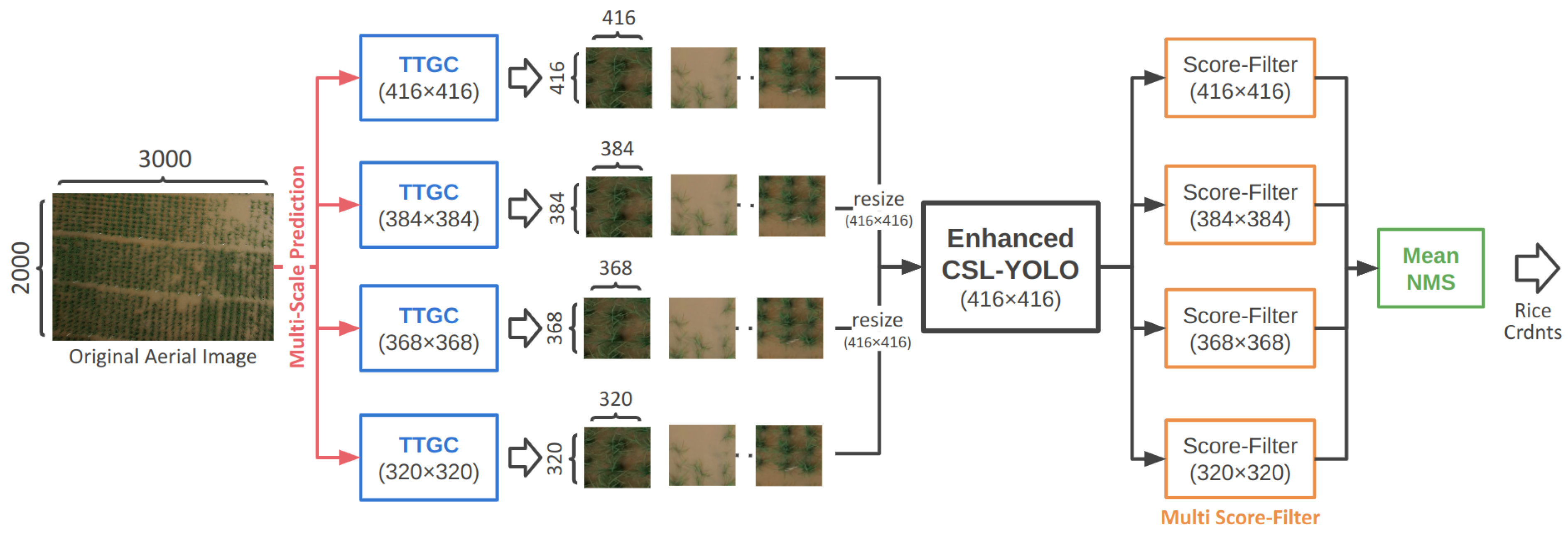
  • Confronted with high-resolution aerial images and rice plants exhibiting a substantial size disparity, we introduced a tailored grid cropping method, namely testing time grid cropping (TTGC), which significantly elevated the performance of the detector during the testing phase.
  • Beyond TTGC, we integrated additional data augmentation techniques, including multi-scale prediction (MSP), mean-NMS, and multi score-filter (MSF), during the testing phase. These enhancements further bolstered the capability of enhanced CSL-YOLO to detect densely packed small rice plants.

2. Related Work

2.1. Machine Learning in Agricultural Applications

In the existing literature, there are various approaches for the application of machine learning to the field of agriculture. For instance, methods based on random forests and Markov random fields have been employed for plant classification in studies such as [8,9,10]. In recent years, a shift towards deep learning methodologies has become evident, as exemplified by [1], who pioneered the use of convolutional neural networks (CNN) for plant segmentation, achieving remarkable results. Building upon this, the study in [11] utilized semantic segmentation for plant counting, while the work in [3] proposed an end-to-end model to streamline the counting process. In the pursuit of efficiency, the study in [4] introduced a lightweight CNN architecture to expedite weed recognition tasks, and the study in [5] extended CNN applications to a broader spectrum of plant identification. Using NIR image along with a CNN, the authors of [12] achieved more accurate identification of target crops and weeds. Furthermore, the study in [2] employed the faster R-CNN framework [13] in a detection-based approach, demonstrating impressive results in precisely localizing fruits. These advancements highlight the evolution in agricultural applications, showcasing a discernible shift from conventional machine learning approaches towards more sophisticated deep learning techniques. In this paper, we focus on recognizing rice plants in aerial images, employing the advanced lightweight CSL-YOLO [14] for plant detection.

2.2. Two-Stage Object Detection

The traditional object detector in deep learning consists of two stages. The first stage involves generating regions of interest (ROIs), and the second stage is inputting these ROIs into a CNN model to extract and classify high-semantic features. This two-stage approach typically yields higher accuracy. However, due to the time-consuming nature of ROI generation and the difficulty in accelerating this process, the overall model runtime is considerably slower than the one-stage method. A RCNN [15] utilizes the selective search algorithm to replace the grid-based method for collecting ROIs, significantly enhancing the speed of the first stage. The faster-RCNN [16] introduces the ROI pooling mechanism, building upon RCNNs. This mechanism eliminates the need for individually passing ROIs generated in the first stage through the CNN backbone. Instead, corresponding features are cropped based on ROIs from a fixed feature map, leading to a substantial increase in the speed of the second stage. The faster-RCNN [13] employs an additional CNN model, referred to as region proposal network (RPN), to replace the selective search algorithm for ROI extraction. This architecture ensures that both stages are composed of CNN models, facilitating GPU parallelization acceleration. Consequently, faster-RCNN can be considered the first high frames per second (FPS) model implemented on advanced GPUs. Various subsequent models have emerged from faster-RCNN, including mask-RCNN [17], which introduced a prediction branch for instance segmentation, and ThunderNet [18], a lightweight two-stage model. In summary, two-stage models typically represent more complex systems, with slower speeds but higher accuracy.

2.3. One-Stage Object Detection

A one-stage object detector removes the stage of generating ROIs and employs a single convolutional neural network (CNN) model to extract features from the input image, yielding multiple object predictions. YOLO [19,20,21,22] utilizes a fully CNN backbone, DarkNet, to output a feature map and directly predicts bounding box positions and classifications through a fully connected layer. While this intuitive method achieves high speeds, this comes at the cost of sacrificed accuracy. YOLO inspired SSD [23], which introduced multi-scale prediction and incorporated the anchor mechanism used by region proposal network (RPN), in addition to employing different label assignment methods. These methods enable SSD to maintain a high speed like YOLO, while significantly enhancing accuracy. Following in the footsteps of SSD, YOLOv2 [20] introduced anchors to YOLO and employed additional techniques to achieve improved accuracy compared to SSD. RetinaNet [24], an extended version based on SSD, identified an issue with one-stage models having too many negative samples due to the absence of an ROI generation stage. This abundance of negative samples hindered loss convergence to the optimal state, prompting the introduction of focal loss. Designed to address this problem, focal loss was coupled with the novel addition of a feature pyramid network (FPN) [25] to SSD [23] for accuracy enhancement. YOLOv3 [21] further integrated a FPN and other techniques to achieve results approaching those of RetinaNet [24]. Subsequently, YOLOv4 [22] added many tricks on top of YOLOv3, to improve accuracy. Additionally, CSL-YOLO [14] emerged as a lightweight and advanced YOLO model. It introduced a lightweight convolution method named CSL-Module as a fundamental component, along with a lightweight backbone and FPN. Specific techniques tailored to CSL-YOLO’s specialized structure were proposed, ultimately improving accuracy. Comparative results on MS-COCO [26] indicated that CSL-YOLO is an advanced lightweight model in the YOLO series, especially compared to the similarly advanced Tiny-YOLOv4. CSL-YOLO achieved a higher detection accuracy, with a smaller footprint and faster processing speed.
CSL-YOLO integrated a myriad of concepts. Their CSL-M incorporates the divide-and-conquer principles from GhostNet [27] and CSPNet [28]. It splits the feature map along the channel axis, with one portion undergoing computationally intensive operations and the other undergoing more cost-effective operations. The bidirectional feature fusion approach in CSL-FPN matches the popular methodologies found in [29,30,31]. Furthermore, according to references [32,33], global features play a crucial role in the effectiveness of CNNs. CSL-FPN addresses this by employing fusion blocks stacked R times, enhancing the model’s ability to capture global features.

3. Proposed Approaches

This chapter presents our proposed methods, encompassing the preprocessing of the training data, which involved systematically processing the original aerial photographs of rice fields. We also delve into the details of the enhanced CSL-YOLO, a robust and lightweight detector meticulously crafted for precise and efficient detection of rice plants. Additionally, we introduce various testing time augmentations strategically designed to address the challenges posed by the small size of rice plants in aerial images. The efficacy of these methods was substantiated through dedicated experiments detailed in a subsequent chapter.

3.1. Training Data Preprocessing

The aerial images from the AI CUP 2021 come in two resolutions: 3000 × 2000 and 2304 × 1728. Each image contains hundreds of rice plants, with experts marking the x and y coordinates of the roots. This entails two challenges. First, the input images are too large, leading to floating point operations (FLOPs), with the parameters required for the model being prohibitively large for most computers. To address this issue, we propose random cropping, dividing the original images into smaller sub-images to keep the model’s resource demands within an acceptable range during the inference of a single image. The second challenge is using an object detection model to determine the bounding box of rice plants. However, the original label set only includes center point coordinates without the width and height of rice plants, and relying on manual labeling for the bounding boxes of hundreds of small-sized rice plants in a single image is impractical and may compromise quality. To overcome this issue, we introduce the semi-supervised labeling binding box, a method to rapidly label bounding boxes for all rice plants in a semi-supervised manner based on marked x and y coordinates, facilitating the training of the detector.

3.1.1. Random Cropping

To address the computational challenges posed by the excessively high resolution in the original images, an intuitive approach would be to directly resize the images to a more manageable resolution. However, considering the diminutive size of a single rice plant in the aerial image, a simple reduction in image size would cause the rice plant’s features to nearly disappear, making them difficult to detect. To tackle this issue, we crop the aerial images into several sub-images, instead of resizing them. During the training stage, we randomly select the starting (x, y) coordinates in the image and crop a region ranging from 256 to 768, creating a sub-image of the original. After repeated random cropping, a set of sub-images is formed, which are then resized to the model’s input size (e.g., 224 × 224, 416 × 416, …) following data augmentation during training. Simultaneously, the (x, y) coordinates of the rice plant roots in these sub-images are synchronously updated to new coordinates. Consequently, each sub-image and contained rice plant becomes independent training data, eventually fed into the CSL-YOLO for training. However, random cropping cannot be used during the testing stage, as this may lead to disregarding certain areas containing rice plants.Fixed grids are employed instead of random cropping, to ensure the accurate representation of each rice plant in the sub-images. This method will be further elaborated in the subsequent sections.

3.1.2. Semi-Supervised Labeling Bounding Box

The original AI CUP 2021 dataset included annotations for the root coordinates of each rice plant in aerial images. However, annotating the bounding boxes of the rice plants is essential to train an object detection model. Given the immense number of rice plants in the aerial images, manually labeling all instances would be a time-consuming task, demanding significant human resources. Previous studies [34,35,36] have introduced semi-supervised training methods based on neighborhood relationships between features, showcasing remarkable achievements. Inspired by this, we propose a simple and intuitive semi-supervised annotation method. In this approach, we initially manually label a few bounding boxes for randomly chosen rice plants in an aerial image. Subsequently, we utilize the maximum and minimum height and width values from these manually labeled bounding boxes as upper and lower bounds. Random values within these bounds are then assigned to the remaining unlabeled rice plants. Figure 2 shows the visual demo, and the entire method can be succinctly expressed through the following formula:
D = { d 0 , d 1 , , d n } ,
The set D encompasses the (x, y) coordinates labeled in the AI CUP 2021 dataset, while the variable d refers to all the data within D, amounting to a total of n entries.
M = { m 0 , m 1 , , m k } , k n ,
First, we randomly select k samples from the dataset D and use manual labeling to create the set M. The value of k is intentionally kept small, typically ranging between 10 and 20 in practical scenarios.
b i = [ d i x , d i y , r a n d ( M m i n w , M m a x w ) ) , r a n d ( M m i n h , M m a x h ) ) ] , B = { b 0 , b 1 , , b i , , b n } .
Ultimately, we leverage the artificially labeled set M to create semi-supervised bounding boxes. Specifically, we calculate the maximum and minimum widths based on the artificially labeled data. Subsequently, these two values serve as upper and lower bounds for randomly generating the width and height of bounding boxes for  D M . This process is applied identically to both width and height. Consequently, for an original sample  d i , its corresponding bounding box  b i  is defined as [ d i x , d i y , rand ( M min w , M max w ) , rand ( M min h , M max h ) ]. The ultimate collection set, denoted as B, constitutes the dataset for training CSL-YOLO.

3.1.3. Random Affine Operations for Training

After subjecting the original images to random cropping and semi-supervised labeling of bounding boxes, they are transformed into a set of sub-images. These sub-images constitute the training data for our object detection model. In order to enhance the robustness of the detector, diverse affine operations are incorporated during the training stage. Rotation, padding, flipping, mix-up, and other operations are randomly applied to each sub-image. The entire process is executed online, and each iteration involves new random affine operations. An affined image is depicted in Figure 3.

3.2. Enhancing CSL-YOLO for Accurate Detection

We utilized random cropping to decrease the dimensions of the original images. Furthermore, we adopt a semi-supervised methodology to generate bounding boxes based on the root coordinates of the rice plants. As a result, our developed object detection model is specialized for identifying rice plants. This model is an adaptation of CSL-YOLO, which prioritizes lightweight design and has demonstrated remarkable performance on MS-COCO in previous experiments. To better suit the requirements of rice plant detection, we made specific modifications to different components of the model, which will be elaborated on in the following sections. The overall architecture of the enhanced CSL-YOLO is shown in Figure 4.

3.2.1. Bigger Backbone

The original CSL-YOLO employed CSL-Bone as the backbone. CSL-Bone is an extremely lightweight backbone, compared to the VGG or ResNet, but it exhibited limitations in capturing image features effectively in experiments [14] on CIFAR-10. In light of this, we conducted a reassessment of the detection accuracy and FLOPs. Considering that speed is not the primary concern in our research, we decided to substitute CSL-Bone with another lightweight backbone, EfficientNet-B1 [38], which offers slightly higher FLOPs but boasts superior accuracy. This choice was made to ensure that the model possesses a more substantial capability to capture the distinctive characteristics of the image.

3.2.2. Bigger FPN

CSL-FPN is an extension component introduced in CSL-YOLO that employs a unique cross-layer fusion technique, which achieves more efficient scale feature fusion with fewer convolutional layers. This method relies on two crucial parameters: Filters and R. Filters determine the final number of channels in the output layer for each scale in CSL-FPN. The default is set at 112, and we increased this to 128 through increasing minor FLOPs to bolster the feature expression capability of CSL-FPN. The parameter R is also used by CSL-YOLO [14] to signify the total number of fusion blocks in CSL-FPN. Their experiments on MS-COCO revealed that increasing R results in a slower speed but improved detection accuracy. Thus, they set R to 3, for a trade-off between FLOPs and mAP. In pursuit of more robust performance, we slightly elevated R to 4, to stack four fusion blocks in CSL-FPN; whereby, the detection performance was concurrently heightened with a small increase in FLOPs.

3.2.3. Fully Soft-NMS

The original CSL-YOLO incorporated a variant of the non-maximum suppression (NMS) technique to address overlapping prediction bounding boxes, combining elements from Soft-NMS [39] and traditional NMS. A threshold value, denoted as t, is introduced. In cases where two bounding boxes exhibit overlap, if the intersection over union (IoU) surpasses the threshold, the box with the lower confidence score is directly eliminated—a scenario analogous to standard NMS. Conversely, if the IoU is less than or equal to the threshold, the confidence score of the lower-scoring box is further attenuated, akin to Soft-NMS. Given the utilization of the multi-scale prediction strategy during the testing time augmentation (TTA) phase, which implements our proposed Mean-NMS, we aimed to minimize the bounding box loss at this stage. This approach ensures the preservation of more boundaries during TTA. Consequently, we set the threshold t to 1, making this hybrid NMS equivalent to Soft-NMS.

3.3. Testing Time Augmentation (TTA)

In addition to enhancing CSL-YOLO to improve its ability to detect rice plants, a series of data augmentations during the testing time were essential, and we call them testing time augmentations (TTA). First, we introduced testing time grid cropping (TTGC), to address the issue of random cropping, which can lead to missing rice plants on the margins. Subsequently, multi-scale prediction (MSP) was incorporated to enhance the detector’s adaptability for four small to large scales of input images. Furthermore, we proposed a weighted non-maximum suppression method called Mean-NMS to tackle the zero-sum problem associated with traditional NMS. Finally, the proposed multi score-filter (MSF) can fine-tune multiple sets of post-processing parameters for different input scales to maximize the performance of Enhanced CSL-YOLO. The proposed inference procedure consists of Enhanced CSL-YOLO, and the testing time augmentations (TTA) are shown in Figure 5.

3.3.1. Testing Time Grid Crop (TTGC)

During the training stage, we employ a random selection process for the initial (x, y) coordinates and scale, ranging from 224 to 762, to crop original images into smaller sub-images. In the testing stage, to mitigate the risk of missing rice plants caused by random cropping, we utilize a fixed grid method. However, fixed grid cropping may overlook marginal plants, necessitating the careful trimming of margins to address this concern. The cropping process is segmented into main grids and supplementary grids, as illustrated in Figure 6. The supplementary grids serve to complement the edges of the main grids, ensuring that no rice plant is inadvertently cut off at the margins. In practical implementations, we specify the grid sizes to be cut. If the image’s height and width are not divisible, a black border is added to the edges until the image’s scale becomes divisible.

3.3.2. Multi-Scale Prediction (MSP)

The AI CUP 2021 dataset includes images of two different resolutions. Moreover, the aerial images vary in distance, angle, and sunlight, leading to slight differences in the relative proportions of the rice plants in each image. To enhance the detector’s adaptability to diverse scales of rice plant, the proposed multi-scale prediction (MSP) utilized TTGC to divide the original aerial images, specifying four width and height dimensions, ranging from 320, 368, 384, and 416. Subsequently, the divided images are resized to the detector’s input scale (416 × 416) for prediction. Figure 5 shows the details of MSP, MSP enables the detector to capture features at different scales during the prediction, thereby boosting its performance in detecting rice plants.

3.3.3. Mean-NMS for Root Coordinate

Due to the generation of numerous overlapping bounding boxes by TTGC and MSP, it becomes essential to apply an additional algorithm for post-processing, similar to NMS, to filter out redundant bounding boxes. However, the bounding box with the highest score of those generated by TTGC and MSP may not always represent the optimal choice. Therefore, using NMS to retain only the highest score can significantly diminish the impact of TTGC and MSP. Instead of employing NMS, Soft-NMS can be utilized to penalize the scores of overlapping bounding boxes. Nonetheless, this approach may lead to an excess of final redundant bounding boxes. To address this challenge, we propose a novel approach namely Mean-NMS, which involves a voting NMS with weights. Mean-NMS establishes a threshold value t in a manner similar to NMS. If the intersection over union (IoU) of two overlapping bounding boxes exceeds t, these boxes are grouped together. The scores of the members within each group are then employed as weights to calculate the weighted center points of the cluster. These center points represent the root coordinates of the final predicted rice plants, as illustrated in the accompanying Figure 7. The entire process of Mean-NMS is outlined as follows:
B = { b 0 , b 1 , , b n } ,
The set  B  denotes the predicted bounding boxes, where each  b i  represents a bounding box predicted by the detector in an image. The range from  b 0  to  b n  encompasses numerous bounding boxes that exhibit significant overlap with each other.
g i = { I o U ( b i , b j ) > t | b B } , 0 < t 1 , G = { g 0 , g 1 , , g k } , k n ,
The symbol G signifies a collection of bounding box groups clustered based on IoU (intersection over union), with each  g i  representing a group composed of bounding boxes where the IoU exceeds a specified threshold t.
D = { j = 0 s i z e ( g i ) ( g i , j c o n f i d e n c e × g i , j c e n t e r ) s i z e ( g i ) | g i G } .
D  refers to the set of central coordinates representing the final predictions of the detector for rice plants. Each  d i  signifies a final predicted (x, y) coordinate of a rice plant. The computation involves taking the weighted average of bounding box centers  g i , j  within each  g i . In this process, the center of each bounding box is multiplied by its confidence score. Each  d i  is obtained through this calculation, contributing to the formation of the set  D .

3.3.4. Multi Score-Filter (MSF)

In the CSL-YOLO framework, as in the other YOLO-like frameworks, a set of filters is employed to sift out frames with inadequate dimensions; those either too small or surpassing the image boundaries. CSL-YOLO also discards predicted bounding boxes with confidence levels below a specified threshold after the non-maximum suppression (NMS) step, addressing overlaps. As multi-scale prediction (MSP) is used to generate outputs at different scales for a single image, it becomes apparent that a uniform score threshold across all scales is not optimal. To address this, we propose the multi score-filter method, which customizes the confidence and other value thresholds based on the output scale. Figure 5 shows this concept.

4. Experiments

In the previous sections, we introduced the proposed methods, which include the data preprocessing, the enhanced CSL-YOLO, and various augmentations during the testing time. In this chapter, we divide the experiment into two parts. In the first part, we conducted ablation studies for the proposed methods, to show that these changes were effective. In the second part, we compared the proposed model with other advanced models, to demonstrate that our proposed model is better. The dataset used in this paper was provided by the AI Cup 2021 competition titled “Automatic Marking and Application of Plant Positions in Full-Color Image of Rice Drones”. The training set comprises 44 aerial images, the public test set includes 47 aerial images, and the private test set consists of 50 aerial images. Each image was expertly annotated with the root positions of rice plants. The metric for the dataset assessed whether the proposed methods could accurately predict the coordinates of rice roots in the test data; the correct prediction (x, y) had to fall within a 20-pixel range of the ground truth. The official ground truth for the public/private test sets was not provided, as some results can only be uploaded to the official server during the competition to obtain the F1 score.

4.1. Ablation Studies

As previously mentioned, our capacity for conducting extensive experiments was limited due to the competition’s constraints on result uploads (allowing only five uploads per day). To conduct a more detailed ablation analysis, we divided the existing 44 training data into 34 sub-training data and 10 validation data. In the ensuing ablation experiments, the enhanced CSL-YOLO was trained on the sub-training data and assessed on the validation data.

4.1.1. Enhanced CSL-YOLO

We conducted an ablation study on the validation set to further assess the effectiveness of enhanced CSL-YOLO for detecting rice plants by increasing the model’s size at the expense of FLOPs. This study aimed to observe the detector’s performance both before and after implementing the enhancement modifications. The enhancement of CSL-YOLO involved three key elements. First, we replaced the backbone from CSL-Bone with EfficientNet-B1. Second, we elevated the filters of the feature maps extracted from the backbone from 112 to 128. Third, we increased the hyperparameter R, representing the number of fusion blocks in FPN, from 3 to 4. Ablation experiments were individually performed for each of these components. As illustrated in Table 1, the results showed a 0.3% increase in F1 after replacing the backbone, followed by an additional 0.2% improvement upon increasing the filters. Raising R to 4 resulted in a further increase of 0.5%. Furthermore, we observed that the detector’s performance plateaus when R was set to 5. Even with a more robust backbone like EfficientNet-B3 and an increased filter size of 144, the performance declined. This result showed that the performance gains achievable through enlarging the model had reached saturation. Therefore, based on this insight, we proposed a series of testing time augmentations. The outcomes of the ablation experiments highlighted the effectiveness of the modifications implemented in the proposed Enhanced CSL-YOLO. Although also increasing the FLOPs, it is essential to note that speed is not the primary goal of this paper.

4.1.2. Testing Time Augmentation (TTA)

We employed various data augmentation techniques for testing time, and the proposed TTA consisted of TTGC, MSP, Mean-NMS, and MSF. To assess their effectiveness, we conducted ablation experiments to evaluate the impact of each proposed augmentation method during testing. The experimental results are presented in Table 2. First and foremost, TTGC demonstrated the most significant performance improvement, with the F1 score showing a notable increase of 10.3%. This is attributed to the substantial scale gap between the original aerial images and rice plants mentioned earlier, and TTGC effectively addressed this issue in a grid cropping. Furthermore, MSP captured multi-scale rice features, resulting in an additional 0.8% F1 gain. When combined with Mean-NMS and MSF, an additional 0.6% F1 gain was achieved. Collectively, the proposed TTA methods contributed to a remarkable 12.7% F1 improvement, enabling Enhanced CSL-YOLO to exhibit impressive performance in rice detection.

4.2. Compared to Other Methods

The results presented in Table 1 clearly demonstrate that minor modifications to the original CSL-YOLO improved the detection performance for rice plants. Our proposed testing time augmentation (TTA) methods addressed specific challenges and contributed to notable performance enhancements, including TTGC, MSP, Mean-NMS, and MSF. TTGC overcame issues related to small rice proportions and potential losses due to fixed grid cropping, while MSP handled varied lighting and scale challenges in different scenes. Mean-NMS improved the bounding box selection, and MSF enhanced the detector performance across various input sizes with multiple post-processing hyperparameter sets. To further evaluate our Enhanced CSL-YOLO + TTA, we compared it with other state-of-the-art models using the AI CUP 2021 public test set. U-Net(LOWBB) [6] and CSRNet [7] were chosen as baseline models, relying solely on x and y coordinates as inputs with heat maps, requiring extensive upsampling and resulting in a slower execution. We expanded the comparison by enhancing U-Net(LOWBB) with backbone variations from EfficientNet-B0 to EfficientNet-B7 [38] and creating an ensemble of CSRNet. The detailed comparison results in Table 3 indicate our method outperformed the others by 4.6% and 2.2%, respectively, highlighting the significant superiority of our proposed approach. The introduced improvements in detecting central rice plant coordinates, including a more efficient detector and a range of TTA methods, contributed significantly to our method’s enhanced performance compared to the baseline approaches.

5. Conclusions

In this paper, we first discussed the detection problem of the original aerial images of the AI Cup 2021, which are excessively high resolution. Then, we introduced a series of preprocessing steps, wherein the original aerial images are cropped into multiple sub-images at random positions and scales, and then the proposed semi-supervised labeling method generates bounding boxes of sub-images. Finally, we employ several random affine operations to augment the sub-images, such as rotation, flip, and mixup, to enhance the robustness of the detector in dynamic agricultural environments. In addition, we prioritized performance over speed by expanding the backbone and FPN to improve the original CSL-YOLO; in other words, we make a trade-off by sacrificing a little speed to enhance the detection. This trade-off significantly improved the performance of CSL-YOLO in our ablation study. To further boost the proposed “Enhanced CSL-YOLO’s performance, we incorporated the TTA methods, including TTGC, MSP, Mena-NMS, and MSF”. Finally, the proposed “Enhanced CSL-YOLO w/ TTA” outperformed two other advanced methods (UNet, CSRNet) that rely on large-scale upsampling for segmentation in terms of F1. In summary, we presented a detection model for detecting the center coordinates of rice plants, and impressive results were achieved on the AI CUP 2021 dataset when adding the proposed TTA methods. The Figure 8 provides additional visualizations of the detected root coordinate results.

Author Contributions

Conceptualization, Y.-M.Z. and C.-C.L. and C.-H.C.; methodology, Y.-M.Z. and C.-C.L.; software, Y.-M.Z.; validation, Y.-M.Z. and C.-C.L.; formal analysis, Y.-M.Z.; investigation, Y.-M.Z.; resources, C.-C.L. and C.-H.C. and K.-C.F.; data collection, Y.-M.Z.; writing—original draft preparation, Y.-M.Z. and C.-C.L.; writing—review and editing, Y.-M.Z. and C.-C.L.; visualization, Y.-M.Z.; supervision, C.-C.L. and C.-H.C.; project administration, C.-C.L.; funding acquisition, K.-C.F. All authors have read and agreed to the published version of the manuscript.

Funding

This research was funded by the National Science and Technology Council under grant number MOST 110-2221-E-008-055-MY3, Taiwan, R.O.C.

Data Availability Statement

The dataset utilized in this paper was made available through the AI CUP 2021 competition. You can access the competition details via the following hyperlink: https://reurl.cc/2zKjQr. This website provides comprehensive information about the competition, including details about the organizing laboratory.

Conflicts of Interest

The authors declare no conflict of interest.

Abbreviations

The following abbreviations are used in this manuscript:
CNNConvolutional Neural Network
FPNFeature Pyramid Network
FLOPsFloating Point Operations
NMSNon-Maximum Suppression
TTATesting Time Augumentation
TTGCTesting Time Grid Cropping
MSPMulti-SCale Prediction
MSFMulti Score-Filter

References

  1. Bargoti, S.; Underwood, J.P. Image segmentation for fruit detection and yield estimation in apple orchards. J. Field Robot. 2017, 34, 1039–1060. [Google Scholar] [CrossRef]
  2. Sa, I.; Ge, Z.; Dayoub, F.; Upcroft, B.; Perez, T.; McCool, C. Deepfruits: A fruit detection system using deep neural networks. Sensors 2016, 16, 1222. [Google Scholar] [CrossRef]
  3. Liu, X.; Chen, S.W.; Liu, C.; Shivakumar, S.S.; Das, J.; Taylor, C.J.; Underwood, J.; Kumar, V. Monocular camera based fruit counting and mapping with semantic data association. IEEE Robot. Autom. Lett. 2019, 4, 2296–2303. [Google Scholar] [CrossRef]
  4. McCool, C.; Perez, T.; Upcroft, B. Mixtures of lightweight deep convolutional neural networks: Applied to agricultural robotics. IEEE Robot. Autom. Lett. 2017, 2, 1344–1351. [Google Scholar] [CrossRef]
  5. Mortensen, A.K.; Dyrmann, M.; Karstoft, H.; Jørgensen, R.N.; Gislum, R. Semantic segmentation of mixed crops using deep convolutional neural network. In Proceedings of the CIGR-AgEng Conference, Aarhus, Denmark, 26–29 June 2016; pp. 26–29. [Google Scholar]
  6. Ribera, J.; Guera, D.; Chen, Y.; Delp, E.J. Locating objects without bounding boxes. In Proceedings of the IEEE/CVF Conference on Computer Vision and Pattern Recognition, Long Beach, CA, USA, 15–20 June 2019; pp. 6479–6489. [Google Scholar]
  7. Li, Y.; Zhang, X.; Chen, D. Csrnet: Dilated convolutional neural networks for understanding the highly congested scenes. In Proceedings of the IEEE conference on computer vision and pattern recognition, Salt Lake City, UT, USA, 18–23 June 2018; pp. 1091–1100. [Google Scholar]
  8. Haug, S.; Michaels, A.; Biber, P.; Ostermann, J. Plant classification system for crop/weed discrimination without segmentation. In Proceedings of the IEEE Winter Conference on Applications of Computer Vision, Steamboat Springs, CO, USA, 24–26 March 2014; pp. 1142–1149. [Google Scholar]
  9. Lottes, P.; Hörferlin, M.; Sander, S.; Stachniss, C. Effective vision-based classification for separating sugar beets and weeds for precision farming. J. Field Robot. 2017, 34, 1160–1178. [Google Scholar] [CrossRef]
  10. Lottes, P.; Hoeferlin, M.; Sander, S.; Müter, M.; Schulze, P.; Stachniss, L.C. An effective classification system for separating sugar beets and weeds for precision farming applications. In Proceedings of the 2016 IEEE International Conference on Robotics and Automation (ICRA), Stockholm, Sweden, 16–21 May 2016; pp. 5157–5163. [Google Scholar]
  11. Chen, S.W.; Shivakumar, S.S.; Dcunha, S.; Das, J.; Okon, E.; Qu, C.; Taylor, C.J.; Kumar, V. Counting apples and oranges with deep learning: A data-driven approach. IEEE Robot. Autom. Lett. 2017, 2, 781–788. [Google Scholar] [CrossRef]
  12. Potena, C.; Nardi, D.; Pretto, A. Fast and accurate crop and weed identification with summarized train sets for precision agriculture. In Proceedings of the Intelligent Autonomous Systems 14: Proceedings of the 14th International Conference IAS-14 14, Shanghai, China, 10 February 2017; Springer: Berlin/Heidelberg, Germany, 2017; pp. 105–121. [Google Scholar]
  13. Ren, S.; He, K.; Girshick, R.; Sun, J. Faster r-cnn: Towards real-time object detection with region proposal networks. Adv. Neural Inf. Process. Syst. 2015, 28. [Google Scholar] [CrossRef] [PubMed]
  14. Zhang, Y.M.; Lee, C.C.; Hsieh, J.W.; Fan, K.C. CSL-YOLO: A Cross-Stage Lightweight Object Detector with Low FLOPs. In Proceedings of the 2022 IEEE International Symposium on Circuits and Systems (ISCAS), Austin, TX, USA, 27 May–1 June 2022; pp. 2730–2734. [Google Scholar]
  15. Girshick, R.; Donahue, J.; Darrell, T.; Malik, J. Rich feature hierarchies for accurate object detection and semantic segmentation. In Proceedings of the IEEE Conference on Computer Vision and Pattern Recognition, Columbus, OH, USA, 23–28 June 2014; pp. 580–587. [Google Scholar]
  16. Girshick, R. Fast r-cnn. In Proceedings of the IEEE International Conference on Computer Vision, Santiago, Chile, 7–13 December 2015; pp. 1440–1448. [Google Scholar]
  17. He, K.; Gkioxari, G.; Dollár, P.; Girshick, R. Mask r-cnn. In Proceedings of the IEEE International Conference on Computer Vision, Venice, Italy, 22–29 October 2017; pp. 2961–2969. [Google Scholar]
  18. Qin, Z.; Li, Z.; Zhang, Z.; Bao, Y.; Yu, G.; Peng, Y.; Sun, J. ThunderNet: Towards real-time generic object detection on mobile devices. In Proceedings of the IEEE/CVF International Conference on Computer Vision, Seoul, Republic of Korea, 27 October–2 November 2019; pp. 6718–6727. [Google Scholar]
  19. Redmon, J.; Divvala, S.; Girshick, R.; Farhadi, A. You only look once: Unified, real-time object detection. In Proceedings of the IEEE Conference on Computer Vision and Pattern Recognition, Las Vegas, NV, USA, 26 June–1 July 2016; pp. 779–788. [Google Scholar]
  20. Redmon, J.; Farhadi, A. YOLO9000: Better, faster, stronger. In Proceedings of the IEEE Conference on Computer Vision and Pattern Recognition, Honolulu, HI, USA, 21–26 July 2017; pp. 7263–7271. [Google Scholar]
  21. Redmon, J.; Farhadi, A. Yolov3: An incremental improvement. arXiv 2018, arXiv:1804.02767. [Google Scholar]
  22. Bochkovskiy, A.; Wang, C.Y.; Liao, H.Y.M. Yolov4: Optimal speed and accuracy of object detection. arXiv 2020, arXiv:2004.10934. [Google Scholar]
  23. Liu, W.; Anguelov, D.; Erhan, D.; Szegedy, C.; Reed, S.; Fu, C.Y.; Berg, A.C. Ssd: Single shot multibox detector. In Proceedings of the European Conference on Computer Vision, Amsterdam, The Netherlands, 11–14 October 2016; Springer: Berlin/Heidelberg, Germany, 2016; pp. 21–37. [Google Scholar]
  24. Lin, T.Y.; Goyal, P.; Girshick, R.; He, K.; Dollár, P. Focal loss for dense object detection. In Proceedings of the IEEE International Conference on Computer Vision, Venice, Italy, 22–29 October 2017; pp. 2980–2988. [Google Scholar]
  25. Lin, T.Y.; Dollár, P.; Girshick, R.; He, K.; Hariharan, B.; Belongie, S. Feature pyramid networks for object detection. In Proceedings of the IEEE Conference on Computer Vision and Pattern Recognition, Honolulu, HI, USA, 21–26 July 2017; pp. 2117–2125. [Google Scholar]
  26. Lin, T.Y.; Maire, M.; Belongie, S.; Hays, J.; Perona, P.; Ramanan, D.; Dollár, P.; Zitnick, C.L. Microsoft coco: Common objects in context. In Proceedings of the Computer Vision–ECCV 2014: 13th European Conference, Zurich, Switzerland, 6–12 September 2014; Springer: Berlin/Heidelberg, Germany, 2014; pp. 740–755. [Google Scholar]
  27. Han, K.; Wang, Y.; Tian, Q.; Guo, J.; Xu, C.; Xu, C. Ghostnet: More features from cheap operations. In Proceedings of the IEEE/CVF Conference on Computer Vision and Pattern Recognition, Seattle, WA, USA, 14–19 June 2020; pp. 1580–1589. [Google Scholar]
  28. Wang, C.Y.; Liao, H.Y.M.; Wu, Y.H.; Chen, P.Y.; Hsieh, J.W.; Yeh, I.H. CSPNet: A new backbone that can enhance learning capability of CNN. In Proceedings of the IEEE/CVF Conference on Computer Vision and Pattern Recognition Workshops, Seattle, WA, USA, 14–19 June 2020; pp. 390–391. [Google Scholar]
  29. Wang, K.; Liew, J.H.; Zou, Y.; Zhou, D.; Feng, J. Panet: Few-shot image semantic segmentation with prototype alignment. In Proceedings of the IEEE/CVF International Conference on Computer Vision, Seoul, Republic of Korea, 27 October–2 November 2019; pp. 9197–9206. [Google Scholar]
  30. Zhang, Y.M.; Hsieh, J.W.; Lee, C.C.; Fan, K.C. SFPN: Synthetic FPN for object detection. In Proceedings of the 2022 IEEE International Conference on Image Processing (ICIP), Bordeaux, France, 16–19 October 2022; pp. 1316–1320. [Google Scholar]
  31. Tan, M.; Pang, R.; Le, Q.V. Efficientdet: Scalable and efficient object detection. In Proceedings of the IEEE/CVF Conference on Computer Vision and Pattern Recognition, Seattle, WA, USA, 14–19 June 2020; pp. 10781–10790. [Google Scholar]
  32. Dosovitskiy, A.; Beyer, L.; Kolesnikov, A.; Weissenborn, D.; Zhai, X.; Unterthiner, T.; Dehghani, M.; Minderer, M.; Heigold, G.; Gelly, S.; et al. An image is worth 16 × 16 words: Transformers for image recognition at scale. arXiv 2020, arXiv:2010.11929. [Google Scholar]
  33. Singh, A.; Bhambhu, Y.; Buckchash, H.; Gupta, D.K.; Prasad, D.K. Latent Graph Attention for Enhanced Spatial Context. arXiv 2023, arXiv:2307.04149. [Google Scholar]
  34. Chen, X.; He, K. Exploring simple siamese representation learning. In Proceedings of the IEEE/CVF Conference on Computer Vision and Pattern Recognition, Nashville, TN, USA, 20–25 June 2021; pp. 15750–15758. [Google Scholar]
  35. Dwibedi, D.; Aytar, Y.; Tompson, J.; Sermanet, P.; Zisserman, A. With a little help from my friends: Nearest-neighbor contrastive learning of visual representations. In Proceedings of the IEEE/CVF International Conference on Computer Vision, Montreal, QC, Canada, 10–17 October 2021; pp. 9588–9597. [Google Scholar]
  36. Biswas, M.; Buckchash, H.; Prasad, D.K. pNNCLR: Stochastic Pseudo Neighborhoods for Contrastive Learning based Unsupervised Representation Learning Problems. arXiv 2023, arXiv:2308.06983. [Google Scholar]
  37. Zhang, H.; Cisse, M.; Dauphin, Y.N.; Lopez-Paz, D. mixup: Beyond empirical risk minimization. arXiv 2017, arXiv:1710.09412. [Google Scholar]
  38. Tan, M.; Le, Q. Efficientnet: Rethinking model scaling for convolutional neural networks. In Proceedings of the International Conference on Machine Learning. PMLR, Long Beach, CA, USA, 9–15 June 2019; pp. 6105–6114. [Google Scholar]
  39. Bodla, N.; Singh, B.; Chellappa, R.; Davis, L.S. Soft-NMS–improving object detection with one line of code. In Proceedings of the IEEE International Conference on Computer Vision, Venice, Italy, 22–29 October 2017; pp. 5561–5569. [Google Scholar]
Figure 1. These two figures present the results obtained by the proposed method on the AI CUP 2021 dataset, which comprises an abundance of rice plants. In the left figure, densely packed green vegetation constitutes individual rice plants and weeds. Due to variations in both the time and location of the captures, the rice in the right figure appears more blurred, being smaller and with increased overexposure, particularly in the central region of the figure. The green dots represent the final predicted coordinates of the rice plant’s positions, and regardless of the image type, the proposed method in this paper exhibited excellent performance.
Electronics 13 00632 g001
Figure 2. These two figures illustrate how the proposed semi-supervised labeling bounding box operates. In the left figure, several bounding boxes are manually selected and labeled. The right figure depicts the bounding boxes generated randomly based on the original root coordinates and the bounding boxes manually labeled a moment previously.
Electronics 13 00632 g002
Figure 3. These two images are training samples that have undergone random affine operations. The process begins with random cropping based on scale, followed by random rotation and padding with random offsets. Finally, the images are combined using mixup [37], where two different images are multiplied by their respective opacities, before synthesis.
Electronics 13 00632 g003
Figure 4. This diagram presents the enhanced architecture of CSL-YOLO, an extension of the original CSL-YOLO framework. CSL-YOLO originally comprised a CSL-Bone as the CNN backbone, CSL-FPN as the neck for multi-scale fusion, and YOLO as the detection head. We upgraded the backbone to the more robust EfficientNet-B1. In the original CSL-YOLO, the feature maps extracted from the backbone underwent a conv-1×1 operation with 112 filters; we increased this to 128 filters. Additionally, we augmented the number of fusion blocks in CSL-FPN from 3 to 4 (R = 4). Finally, all feature maps are passed through the YOLO head to obtain the prediction bounding boxes.All modifications are highlighted in red within the diagram.
Electronics 13 00632 g004
Figure 5. The depicted flowchart illustrates the step-by-step operation of the proposed methods, moving from left to right. Upon inputting an original aerial image, the initial step involves the application of multi-scale prediction (MSP) to perform testing time grid cropping (TTGC) at four distinct scales. Subsequently, all sub-images are resized to 416 × 416 and utilized as input for Enhanced CSL-YOLO to make predictions. Following prediction, the multi score-filter (MSF) is employed to allocate independent hyperparameters for each input size, facilitating the selection of promising bounding boxes. The final step involves using Mean-NMS to yield the predicted coordinates of rice roots in the original aerial image.
Electronics 13 00632 g005
Figure 6. This diagram illustrates how TTGC crops the image. The orange squares represent the main grids, while the remaining blue and green squares indicate the supplementary grids used to fill in the boundaries of the main grids.
Electronics 13 00632 g006
Figure 7. This flowchart illustrates the computation process of the proposed Mean-NMS. The left figure displays two sets (green and red) of overlapping bounding boxes. While traditional NMS retains only the bounding box with the highest confidence, Mean-NMS adopts a weighted average approach to calculate the root coordinates for the AI CUP 2021 evaluation criterion.
Electronics 13 00632 g007
Figure 8. These images showcase rice plants identified through our proposed methodology in a dynamic environment. Each green dot signifies the root coordinates of individual rice plants.
Electronics 13 00632 g008
Table 1. This table illustrates the changes in FLOPs and F1 score of the various components in Enhanced CSL-YOLO before and after replacement. These components include the backbone, the number of filters, and the number of fusion blocks—R.
BackboneFiltersRMFLOPsF1(%)
CSL-Bone1123144179.3
EfficientNet-B11123211279.6
EfficientNet-B11283225079.8
EfficientNet-B11284243480.3
EfficientNet-B11285261880.3
EfficientNet-B31445398680.1
Table 2. This table shows the contribution of each testing time augmentation (TTA) technique to the F1 score. The experiment was conducted on the validation dataset split from the AI CUP 2021 training set.
TTGCMSPMean-NMSMSFF1(%)
----79.3
----80.3
---90.6
---91.4
---80.2
--92.4
--90.6
-92.8
93.0
Table 3. This table compares the proposed Enhanced CSL-YOLO+TTA and two baseline models on the AI CUP 2021 test set.
 F1(%)
U-Net82.0
U-Net w/ EfficientNet-B183.0
U-Net w/ EfficientNet-B385.0
U-Net w/ EfficientNet-B788.2
CSRNet89.6
Ensembled CSRNet92.0
Enhanced CSL-YOLO86.2
Enhanced CSL-YOLO w/ TTA94.2
Disclaimer/Publisher’s Note: The statements, opinions and data contained in all publications are solely those of the individual author(s) and contributor(s) and not of MDPI and/or the editor(s). MDPI and/or the editor(s) disclaim responsibility for any injury to people or property resulting from any ideas, methods, instructions or products referred to in the content.

