Article

Seismic Event Detection in the Copahue Volcano Based on Machine Learning: Towards an On-the-Edge Implementation

by
Yair Mauad Sosa
1,
Romina Soledad Molina
2,3,*,
Silvana Spagnotto
4,5,6,
Iván Melchor
6,7,
Alejandro Nuñez Manquez
1,
Maria Liz Crespo
2,
Giovanni Ramponi
3 and
Ricardo Petrino
1
1
Departamento de Electrónica, Facultad de Ciencias Físico Matemáticas y Naturales, Universidad Nacional de San Luis, San Luis 5700, Argentina
2
Multidisciplinary Laboratory (MLab), Science, Technology and Innovation Unit (STI), The Abdus Salam International Centre for Theoretical Physics, 34151 Trieste, Italy
3
Dipartimento di Ingegneria e Architettura (DIA), Università degli Studi di Trieste, 34127 Trieste, Italy
4
Departamento de Geología, Facultad de Ciencias Exactas y Naturales, Universidad de Buenos Aires, Buenos Aires 1053, Argentina
5
Departamento de Física, Facultad de Ciencias Físico Matemáticas y Naturales, Universidad Nacional de San Luis, San Luis 5700, Argentina
6
Consejo Nacional de Investigaciones Científicas y Técnicas (CONICET), Buenos Aires 1033, Argentina
7
Instituto de Investigación en Paleobiología y Geología (IIPG), Universidad Nacional de Río Negro, General Roca 8332, Argentina
*
Author to whom correspondence should be addressed.
Electronics 2024, 13(3), 622; https://doi.org/10.3390/electronics13030622
Submission received: 30 December 2023 / Revised: 17 January 2024 / Accepted: 31 January 2024 / Published: 2 February 2024

Abstract

:
This study focused on seismic event detection in a volcano using machine learning by leveraging the advantages of software/hardware co-design for a system on a chip (SoC) based on field-programmable gate array (FPGA) devices. A case study was conducted on the Copahue Volcano, an active stratovolcano located on the border between Argentina and Chile. Volcanic seismic event processing and detection were integrated into a PYNQ-based implementation by using a low-end SoC-FPGA device. We also provide insights into integrating an SoC-FPGA into the acquisition node, which can be valuable in scenarios where stations are deployed solely for data collection and holds the potential for the development of an early alert system.

1. Introduction

Continuous monitoring of active volcanoes allows for the ongoing assessment of their internal and external activities, facilitating the detection of anomalies—also known as precursors—that may precede an eruption. Adequate volcanic monitoring by utilizing various techniques and comprehensive analysis of the collected data is essential for precursor detection [1]. Volcano seismology involves the analysis and interpretation of seismic signals generated by active sources inside and around volcanoes, including the application of seismic techniques for imaging internal volcanic structures [2,3].
Technological advancements have led to the widespread use of seismic networks by dedicated observatories for the monitoring of many volcanoes. These observatories automatically collect and analyze continuous data.
A deeper understanding of volcanic behavior can be attained by analyzing volcanic seismic events. Short-Time Average over Long-Time Average (STA/LTA) [4] is a broadly used algorithm that allows the detection of an event through its energy, and it is typically applied to data that undergo bandpass filtering within a frequency range where the signal prevails over the background noise [5]. Nevertheless, for weaker events, the background noise could have a higher amplitude than that of the event itself [6,7]. Additionally, in environments with dynamic noise, no single filter will be universally optimal for a diverse range of signals when using energy detectors [8]. The activation threshold, also known as the trigger, plays a crucial role in determining which events are recorded and which ones are not. Furthermore, experts should set the parameters of STA/LTA methods in such a way that they cannot take advantage of the prior knowledge of previous picks, since each measurement is treated individually [9].
Machine learning (ML) has gained considerable success across various application domains, including image recognition, semantic image segmentation, pest classification, information retrieval, and autonomous driving, among others [10,11,12,13]. Due to the complexity of seismic events, the latest advancements in ML offer powerful solutions for handling large datasets and extracting desired features effectively [14,15]. ML has been employed for event and eruption detection in studies such as [16,17,18]. With the increasing number of seismic sensors deployed for earthquake monitoring, the accurate identification of signal segments that correspond to events and non-events performed on the acquisition node facilitates postprocessing tasks and enhances the overall efficiency of data analysis.
ML techniques have been used to process data in volcanology [19]. The Cotopaxi Volcano (Mexico) was analyzed through unsupervised learning, where the classification of seismic events was achieved using six clustering-based methods [20]. The authors performed feature extraction on the events, each of which was described by an 84-dimensional feature vector, including 13 features from the time domain, 21 features from the frequency domain, and 50 features from the scale domain. Their reduced dataset comprised 668 long-period (LP) and volcano–tectonic (VT) events.
Lara et al. [21] presented feature selection for seismic events produced by the Cotopaxi Volcano. The time and frequency domains were employed to process the seismic signals. Three types of events were classified—LP, VT, and Hybrid (HB)—and good performance for LP and VT was observed. Events in the Ubinas Volcano were analyzed in [22] using empirical mode decomposition and ML techniques. Spectral, time, and cepstral domains were considered for the definition and computation of attributes. Moreover, the proposed approach used a multichannel triaxial sensor to perform classification (vertical, east, and north channels were considered). Event classification was achieved using a multilayer perceptron (MLP), linear discriminant analysis, random forest, and support vector machine.
Witsil et al. [23] proposed the use of unsupervised ML for continuous infrasound analysis of the Stromboli Volcano in Italy. The authors of [24] examined the continuous wavelet transform (CWT) for volcano–seismic spectral analysis for the Santiaguito Volcano in Guatemala. Volcanic seismic events were classified through wavelet scattering transforms [25] that were applied to the Llaima Volcano in Chile.
A machine learning approach was presented by Falcin et al. [26] for events from La Soufrière Volcano in Guadeloupe. The authors used a random forest classifier to perform event discrimination and categorization. From their proposal, the impact of feature reduction from 104 to 14 could be observed. Titos et al. [27] proposed recurrent neural networks (RNNs), long short-term memory (LSTM), and a gated recurrent unit (GRU) to detect and classify continuous sequences of volcanic seismic events at the Deception Island Volcano in Antarctica. A study using DNN architectures for seismic event classification was presented by Canario et al. [28].
Ren et al. [29] proposed the use of ML to describe specific patterns of seismic signals recorded during eruptions in the Piton de la Fournaise Volcano by employing gradient-boosted decision trees for binary classification. Li et al. [9] proposed an attention-based multi-scale UNet for earthquake detection. An EQTtransformer [30] was proposed for the simultaneous detection of earthquake signals and phases (P and S). The architecture was based on an attention mechanism composed of one very deep encoder and three separate decoders. Tottori earthquakes in Japan were employed to test the performance of the model by slicing the continuous data into 1 min windows.
Considering the aforementioned contributions, employing an extensive array of features enables diverse representations of signals, allowing a wealth of information to be captured. Another benefit of feature utilization is the ability to minimize the data dimensionality, preserving crucial information embedded in the signals.
In this paper, we propose a software/hardware co-design for the detection of seismic events in the Copahue Volcano based on digital signal processing techniques and ML, and the complete process is performed on a system (SoC) based on a field-programmable gate array (FPGA) to achieve event classification on the edge. The selection of this platform was due to its low power consumption, real-time processing, high parallelism that can enable the processing of several channels in parallel, and integration with PYNQ to improve productivity when porting the software into a processing system.
We also provide insights into the integration of a low-end SoC into the acquisition node. This approach holds the potential for the development of an early alert system in conjunction with an acquisition system—as a triggering system based on ML for operation on the edge—as an alternative to methods based on the STA/LTA and power spectral density (PSD) algorithms. Moreover, it can prove valuable in other scenarios, such as landslides or rockfalls.
To the best of our knowledge, there is no previous work that jointly achieved the following:
  • Presented a software/hardware co-design for volcanic seismic event detection based on digital signal processing techniques and ML while considering a multichannel approach;
  • Showed the implementation of an event detection process on a system (SoC) based on a field-programmable gate array (FPGA) to provide data about resource utilization, latency, and power consumption;
  • Exposed insights regarding the integration of a low-end SoC device into the acquisition node as an event-triggered system based on ML to operate on the edge; this can prove valuable in other scenarios, such as landslides or rockfalls, where stations are deployed solely for data collection.
In situations where the distribution of seismic stations is sparse due either to low financial resources or difficult access, an on-the-edge detector can improve the monitoring. Also, this approach can be particularly effective in volcanoes that show seismic events with relatively low amplitudes, i.e., when an event is not recorded in all of the stations of the network.
The rest of this paper is organized as follows. Section 2 presents the geological setting, volcanic seismic event detection, and the software/hardware co-design integrated with PYNQ-Z1. Section 3 describes the experiments and their results. Section 4 shows the proposed system for volcanic seismic event detection on the edge, whereas the discussion is presented in Section 5. Finally, Section 6 presents the conclusions.

2. Materials and Methods

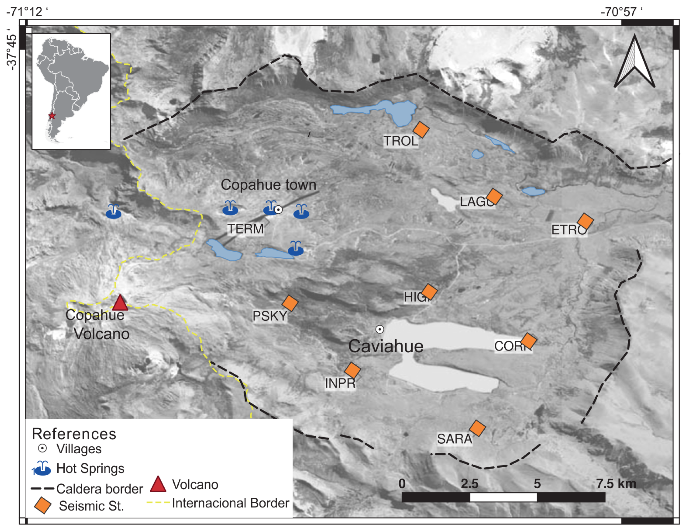
2.1. Geological Setting and Data

The Caviahue–Copahue Volcanic Complex is part of the Southern Volcanic Zone of the Andes and is primarily influenced by the Liquiñe–Ofqui fault system and the Antiñir–Copahue Fault System. The Copahue Volcano is an active stratovolcano situated on the southwest edge of the Caldera del Agrio, a volcanic tectonic depression with a rectangular shape that is oriented NW-SE ([31,32]). It is considered one of the most active volcanoes and is recognized by both Chilean and Argentinian government institutions [33]. The volcano harbors an active geothermal field within the caldera, which is strongly controlled by regional and local tectonics. The summit of the Copahue Volcano is at an altitude of 2997 m. This volcano has experienced numerous eruptions throughout history, with the most recent ones occurring in 2012 and 2000, and fumaroles persist as a product of its permanent activity [34]. Its study is of significant interest due to its geothermal potential, tourism, and the associated volcanic risk.
Between December 2017 and March 2018, the National University of Río Negro deployed a temporary network (called CP) of six broadband and two short-period seismic stations [35]. CP covered an area of 12 km in the East–West (E–W) direction and 14 km in the North–South (N–S) direction in Caldera del Agrio. This network was the result of the collaboration between the National University of Río Negro (Argentina), University of Florence (Italy), Universidad Autónoma de México (México), and University of San Luis (Argentina).
The network of stations was deployed within the Caviahue caldera, providing simpler and less hazardous logistical conditions compared to the slope of the volcano. Special care was taken during the installation of seismometers, which were buried at least one meter deep with a concrete base to minimize ambient seismic noise, consequently enhancing the detection threshold for recorded earthquakes. The stations were strategically located in quiet areas during a period when there were very few people residing in the region. For the study presented in this paper, the seismological station that performed best according to the approach proposed in [35] was selected.
Figure 1 shows the distribution of the stations in the CP network. The stations had triaxial sensors of 20 and 30 s (Nanometrics Trillium Compact 20 s and Guralp 40T 30 s, respectively, Kanata, ON, Canada) and digitizers with storage systems in flash memory and a GPS timing and positioning system (Nanometrics Centaur, Guralp DAS DM-24, and Sara SL06, Kanata, ON, Canada) controlled by a 24-bit A/D converter sampling at 100 Hz. In addition, 100 W solar panels and 105 Ah batteries provided the power for all stations.
The dataset used in this study was composed of raw data acquired from sensors installed at different stations that formed the CP network (the signals used in this research were obtained from Montenegro’s Ph.D. thesis [36] and were provided by “Laboratorio de Estudios y Seguimientos de Volcanes Activos’ (LESVA), Universidad Nacional de Rio Negro). Each station generated signals in vertical, eastern, and northern channels. These files were in the MSEED format (used in seismology to store and distribute time-series data from seismic instrument waveforms), and each was 24 h long, composed of 8,460,000 samples.
Data quality was evaluated in [35], where the noise levels at each station were juxtaposed with Peterson’s global seismic noise models by performing the initial removal of the instrument response. On the other side, the noise levels in all stations remained within the anticipated normal range when no seismic activity was present, as described in [36].
In this study, we focused on the seismic traces recorded at the HIGI station, since more tectonic events were found in proximity to HIGI, and structural models suggested that the magmatic chamber was also situated to the east of the volcanic cone. Moreover, the data quality of the HIGI station was superior to that of TERM, which was possibly due to the presence of geothermal emanations causing noise [35]. Installed at coordinates 37.851° S, 71.030° W and an elevation of 1637 m above sea level, it was situated in the old Hueney campsite. It was positioned on a cement base above a rocky substrate, with an embedding depth of approximately 70 cm. It was composed of a 20-second Trillium Compact sensor controlled by a 24-bit A/D converter sampling at 100 Hz. Also, the HIGI station worked correctly during the entire data acquisition phase. For illustrative purposes, a seismic trace recorded at the HIGI station is shown in Figure 2.

2.2. Volcanic Seismic Event Detection

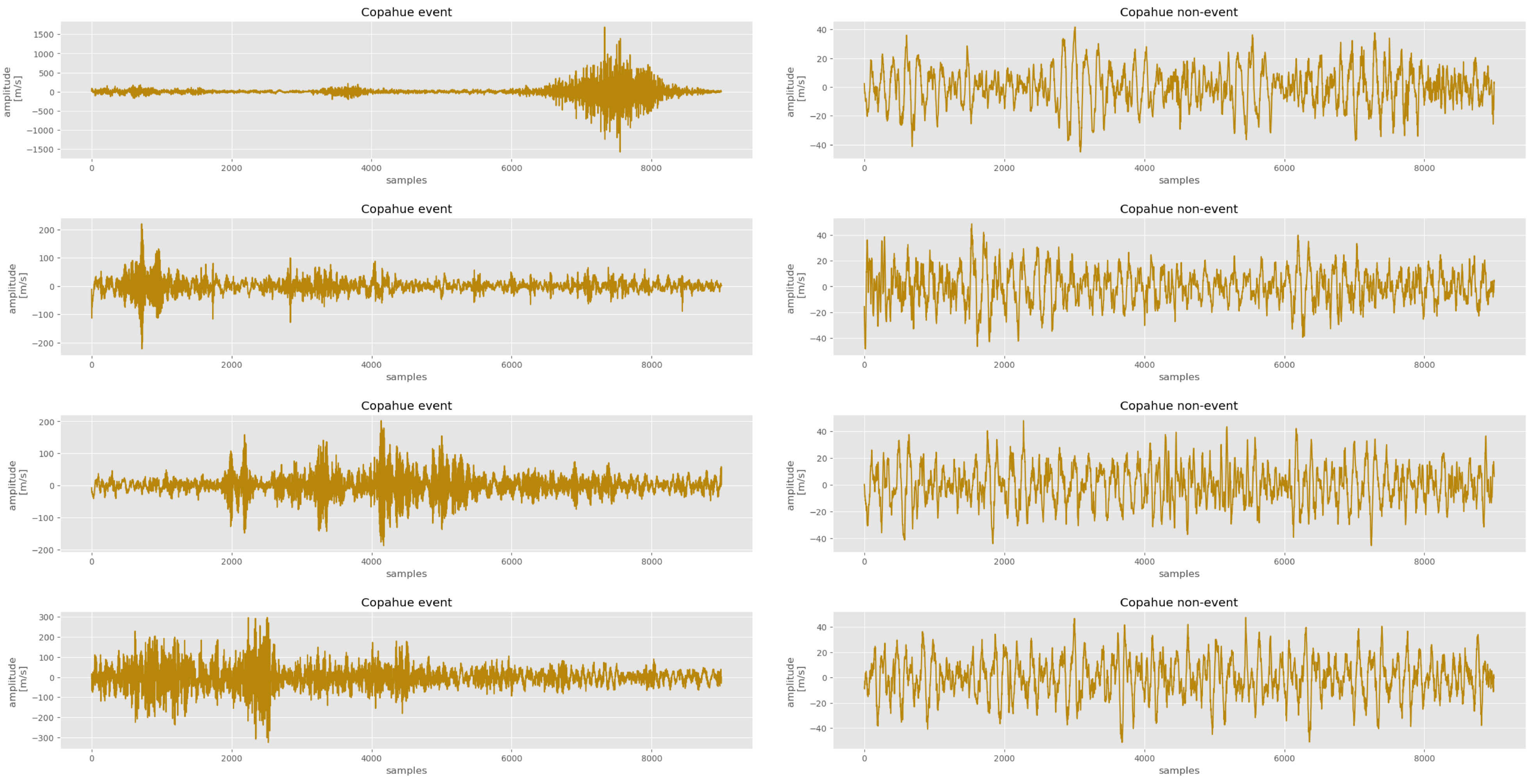
2.2.1. Data Curation and Enrichment

Data curation and enrichment were performed to generate a dataset to train the ML-based model. The 24 h long traces were preprocessed with a Butterworth bandpass infinite impulse response (IIR) filter with order M = 8 [37] applied to the complete trace, with 0.5 Hz and 17 Hz cutoff frequencies. Subsequently, the long traces were trimmed (hereafter referred to as trimmed signal). The corresponding digital cutoff frequencies were fixed at 0.01 and 0.35 rad/sample. Additionally, two bandpass filters defined with cutoff frequencies between 10 Hz and 20 Hz and between 20 Hz and 30 Hz were applied to the clipped signals. The steps of the filtering process are shown in Figure 3. Each IIR filter introduced zero phase distortion, which was achieved through forward and backward filtering [38]. The selected observation time was 1 min 30 s, equivalent to 9000 samples. The time window was chosen based on the duration of the identified volcanic tectonic events.
Feature extraction was accomplished using digital signal processing techniques applied to the trimmed and filtered signals. A total of 66 features were extracted to characterize volcanic tectonic seismic events [39], of which 9 belonged to the time domain, 8 to the frequency domain, and 49 to the scale domain, including the wavelet transform (WT) [24].
The selection of features was based on a state-of-the-art study, drawing from the suggestions made in studies such as [17,20,21,22,26] to aggregate contributions of information from various domains, such as the temporal, frequency, and scale domains. Conversely, feature reduction was proven to be an effective method for training neural networks [26]. In this work, we took advantage of volcanic seismic signal representations through features, aiming to obtain a machine-learning-based model designed for implementation on an edge device.
Feature extraction was performed in the time, frequency, and scale domains.
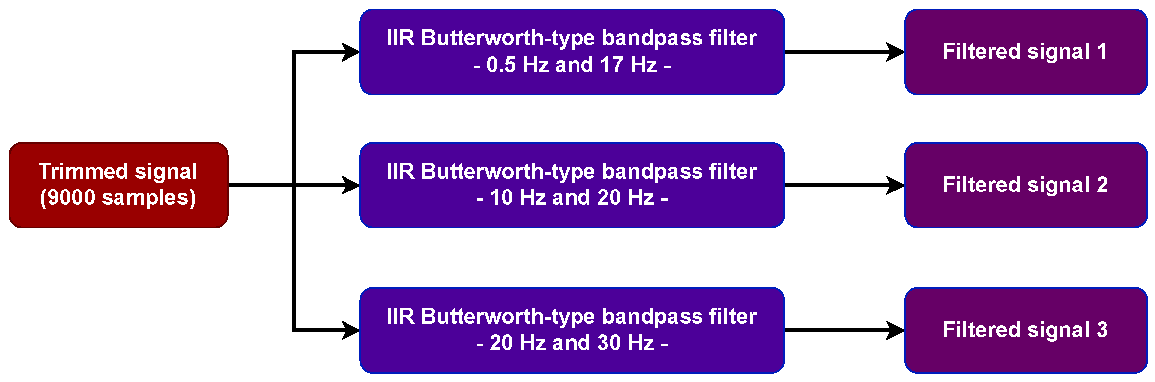
  • Time domain: To obtain features in the time domain, we utilized the filtered traces within the 0.5–17 Hz frequency band.
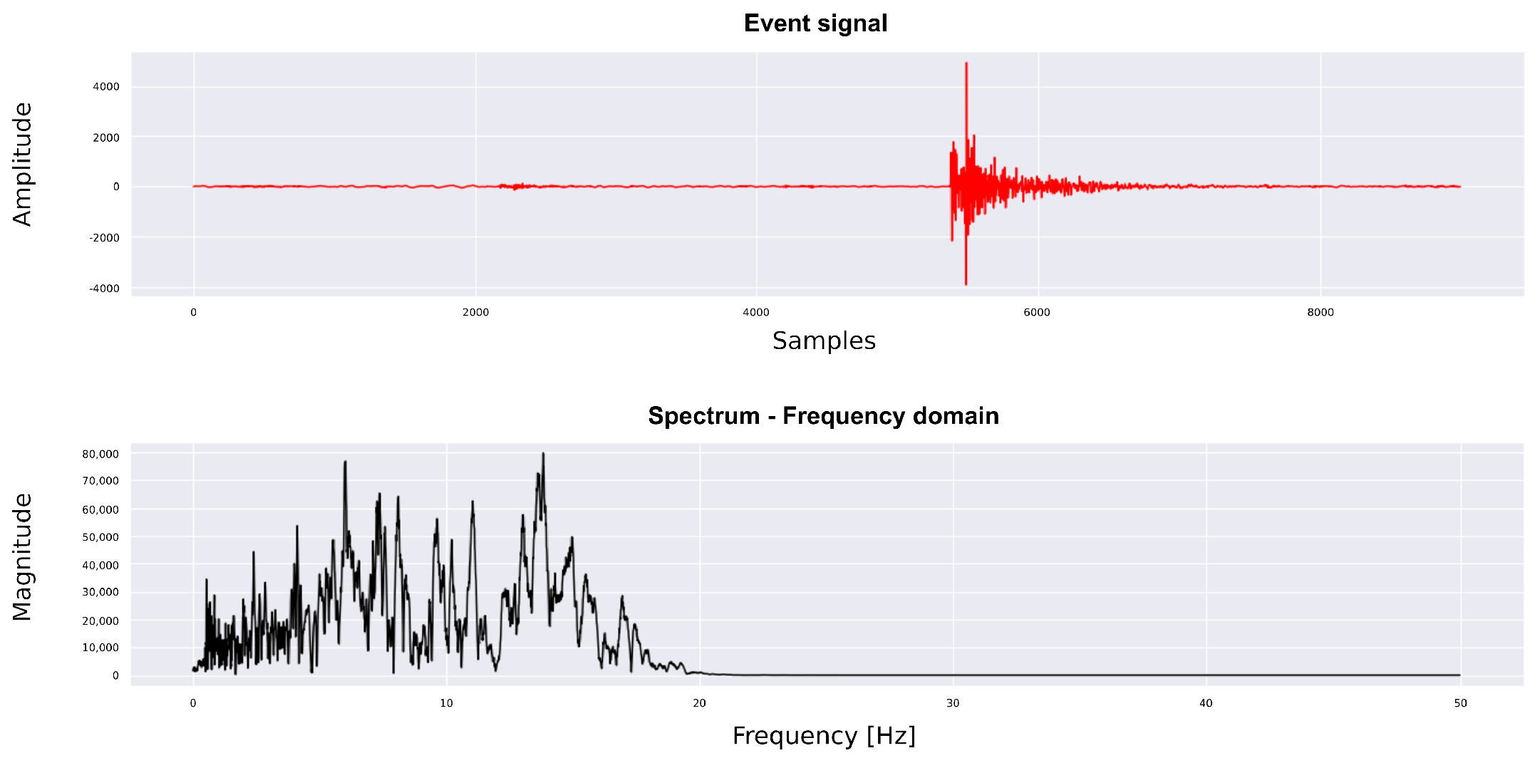
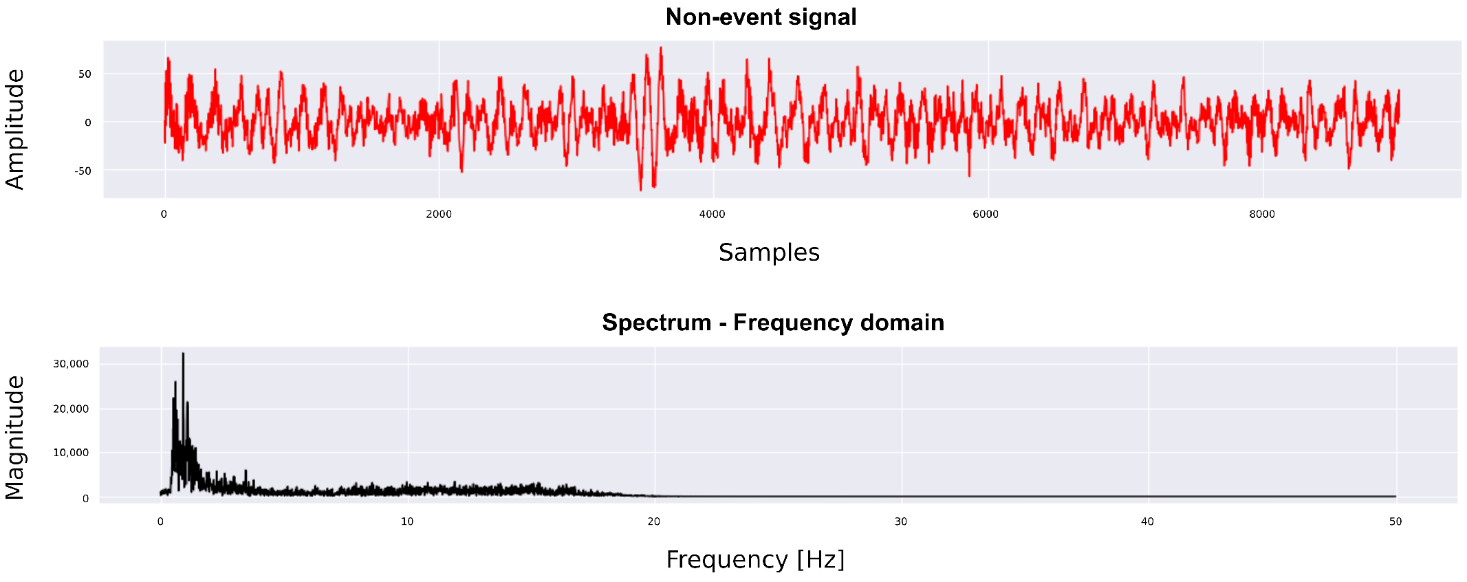
  • Frequency domain: The discrete Fourier transform (DFT) was computed from the signals filtered in the bands 0.5–17 Hz, 10–20 Hz, and 20–30 Hz. After the DFT, various features were extracted.
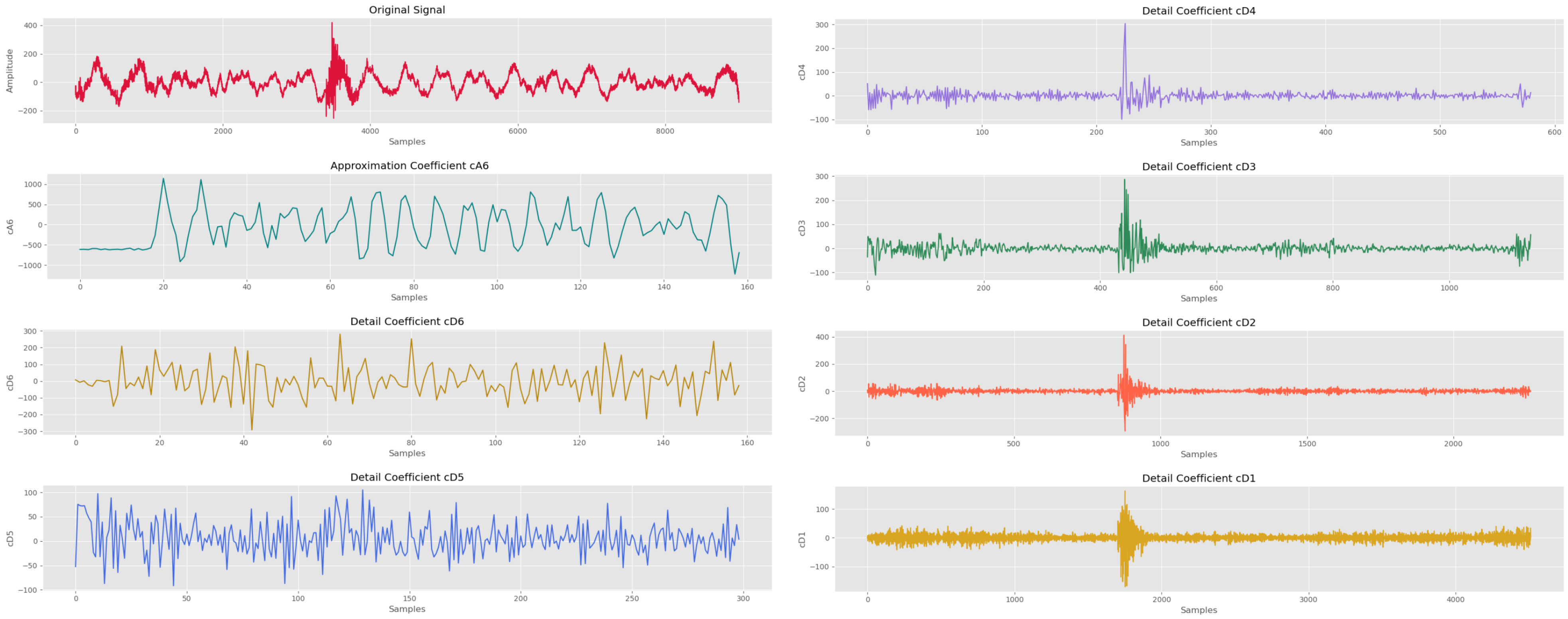
  • Scale domain: The signal was filtered within the frequency range of 0.5–17 Hz and underwent the wavelet transform (WT), resulting in the extraction of approximation and detail coefficients.
The selected features are described below:
  • Average: The sum of a set of values X i , considering i = 1 , 2 , , n , divided by the total number of values n, as shown in Equation (1).
    a v e r a g e ( x ) = x ¯ = 1 n i = 1 n X i
  • Root mean square (RMS): Defined as the square root of the arithmetic mean of the square of data, as shown in Equation (2), where X i is the dataset and n is the total number of data.
    R M S ( x ) = 1 n i = 1 n X i 2
  • Kurtosis: Kurtosis is a measure of the extent of outliers in a dataset. For a normal distribution, the kurtosis statistic has a value of 0. A positive kurtosis indicates that the data exhibit more extreme outliers than a normal distribution. Negative kurtosis indicates that the data have less extreme outliers than a normal distribution. Kurtosis (k) can be obtained using Equation (3), where n is the number of data points, X i is the i-th value of the data, x ¯ is the mean or arithmetic average, and σ is the standard deviation of the dataset.
    k = 1 n i = 1 n ( X i x ¯ ) 4 σ 4
  • Minimum: This is the lowest value that the signal takes within a specific time interval.
  • Maximum: This is the highest value that the signal takes within a specific time interval and is defined by Equation (4), where s ( t ) corresponds to the signal.
    m a x s t = m a x [ s ( t ) ]
  • Time to reach the maximum value: Time taken for the signal to reach its maximum amplitude.
  • Difference between maximum and minimum values of the signal: The difference between the maximum and minimum values of the signal is calculated.
  • Difference between the maximum value and RMS: This is the difference between the maximum value of the signal and its RMS.
  • Energy: Refers to the total amount of energy contained by the signal within a specified time interval. As seen in Equation (5), it is calculated by summing the square of all the signal values X n within a given time interval.
    E x = n = | X n | 2
  • Maximum signal value in the 10–20 Hz frequency band: The highest value of the signal in the frequency domain is calculated for the 10–20 Hz frequency band.
  • Maximum signal value in the 20–30 Hz frequency band: The highest value of the signal in the frequency domain is calculated for the 20–30 Hz frequency band.
  • Maximum frequency value: The value at which the maximum frequency value occurs is obtained. This is performed for the 0.5–17 Hz frequency band.
Considering the wavelet transform, different levels were extracted from the filtered signal (in the 0.5–17 Hz frequency band). The optimal parameters for seismic signal analysis using WT included selecting Daubechies 10 (DB10) as the mother wave and a maximum decomposition level of six [21]. These levels were selected considering the trade-off between the computational cost and the fact that each decomposition served as a filter through which the initial signal needed to pass [21].
Once the mother wave and decomposition levels were determined, several features at each level were computed: the difference between the maximum and minimum, RMS, peak RMS, and percentage of wavelet energy levels. Additionally, the DFT was obtained for each decomposition level to compute the maximum and average values.
Table 1 presents the selected features in the time, frequency, and scale domains.
As a result of this procedure, the curated and enriched dataset comprised trimmed signals, 66 features, and their corresponding classes. However, only the extracted features were used for the training process in this study, and the dataset that was created with the associated raw data opens avenues for future research in this direction.
Furthermore, a feature reduction was carried out using Pearson’s correlation. The values for the correlation coefficients (between the different features) that were equal to or less than 0.2 were kept to eliminate highly correlated variables. This arises from the fact that highly correlated variables are usually redundant and do not offer any extra information to the model. Furthermore, such highly correlated variables may adversely affect the performance of ML algorithms. The result of the reduction through correlation was a streamlined vector consisting of 9 features: kurtosis, peak time, RMS value of wavelet approximation coefficient A6, percentage of energy of wavelet approximation coefficient A6, and percentage of energy in wavelet coefficients D6, D5, D4, D3, and D2.

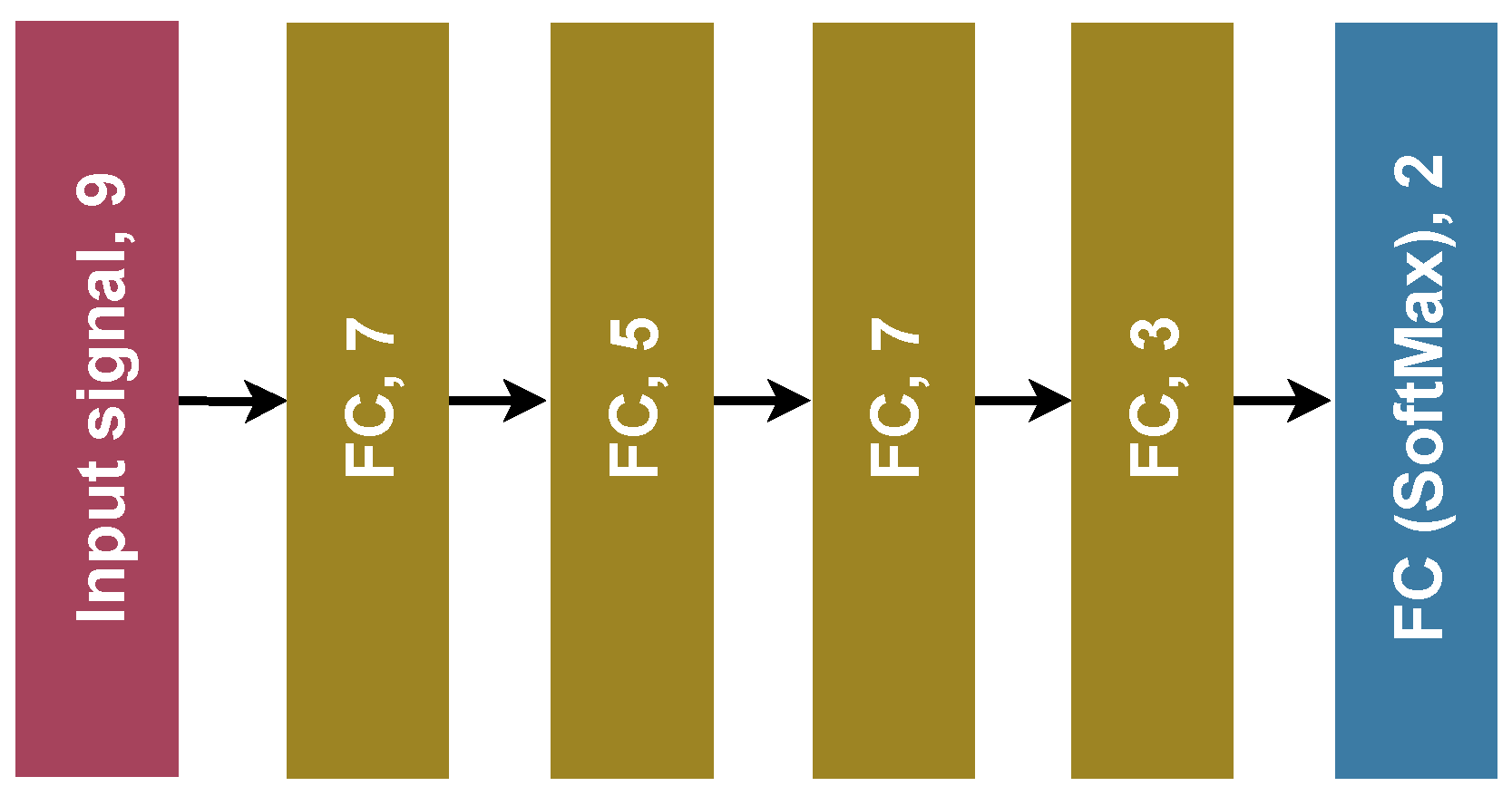
2.2.2. Machine Learning for Event Detection

Because it is desirable to distinguish events from noise signals, a binary classification was proposed using ML as a starting point for further discrimination among various types of events. Examples of the events and noise signals are shown in Figure 4. This group of events comprises volcanic tectonic and tremor signals. The dataset generated for training comprised 15,052 entries that included the extracted features and the corresponding classes (divided into event and non-event). We employed a well-balanced dataset to prevent the model from being biased towards the class with a higher number of elements. A multichannel approach was employed for binary classification, which implied that the signals used for training, validation, and testing were obtained from each channel: vertical, eastern, and northern.
We performed volcanic seismic event classification by training a multilayer perceptron (MLP) model using the resulting dataset, which was split into training (85%) and validation (15%). A total of 300 events and non-events were separated and used solely as a testing set (hereinafter referred to as the TestHIGI dataset).
Furthermore, an extra dataset (hereinafter referred to as the TestNoHIGI dataset) was created to evaluate the inference stage and the ability of the ML-based architecture to generalize. It was composed of signals obtained from the other stations (such as CORR, TROL, ETRO, TERM, and PSKY) that are part of the Cophaue network, which can be observed in Figure 1. When an event occurs, it should be present in at least 3 of the other stations, which means that the event will be present in the stations but with different arrival times and magnitudes because of the signal propagation. For this reason, we performed a first attempt to observe how the model behaved with the TestNoHIGI dataset.
In [36], a list was presented based on the days and times of events that were manually classified. In this study, we used some of these reported events to create an additional testing set. Traces were extracted from the original signals at the time of the event and filtered using the same methodology as explained in the previous sections, incorporating different stations and channels. This resulted in a testing dataset comprising 900 events. The same methodology was applied to non-events, considering that the time and day taken are not listed above. A total of 1800 entries composed the TestNoHIGI dataset.
As our goal was to utilize a low-end SoC based on an FPGA as the edge platform, we employed compression techniques to achieve a smaller and faster MLP-based model without compromising event detection accuracy [40]. The compressed version of the detector resulted from the combined implementation of quantization (8-bit fixed-point), pruning (target sparsity of 25%), and quantization-aware pruning. This corresponded to a segment of the workflow outlined by [41].
The MLP architecture consisted of four hidden layers, as shown in Figure 5. The total number of parameters was 214. This configuration was obtained through hyperparameter optimization using Bayesian optimization [41]. The network was defined using QKeras [42], which supports the definition and training of quantized layers and avoids post-training quantization. Each dense layer employed ReLu as an activation function, and softmax was applied to the output layer. The optimizer was set to Adam with a learning rate of 0.001. The number of epochs and the batch size were both fixed at 32.

2.3. Software/Hardware Co-Design and PYNQ Framework

The open-source PYNQ framework [43], built upon the Xilinx SoC and MPSoC technologies, facilitated the utilization of the board’s FPGA part in Python applications. This approach empowers FPGA-based IP designers to present their optimized functions in a user-friendly manner, similarly to software libraries, thereby ensuring an effortless integration. PYNQ offers a collection of integrated software and hardware components, allowing the utilization of existing elements directly and modifying/expanding functionality as required.
A software/hardware co-design was performed and integrated into the PYNQ framework to achieve volcanic seismic event detection. The feature extraction task was developed on the processing system side, composed of an ARM Cortex-A9 dual-core, whereas the ML-based classifier was implemented in the FPGA part. Figure 6 shows the different components of the overall system.

2.3.1. Hardware Platform Creation

The ML-based inference hardware block was obtained through a high-level synthesis (HLS) tool using high-level synthesis for machine learning (hls4ml) [44], which is an open-source software package for mapping ML-based inference into an HLS project, generating the hardware block to perform the classification task.
After the ML-based model training and compression, the model was saved in .h5 format. This type of file was the input for the hls4ml package to translate the ML-based model into an HLS project. In the hls4ml configuration, the reuse factor variable was set to 1, and the latency was chosen as the optimization strategy. The former enabled the utilization of multipliers in the FPGA for the multiply–accumulate operations. Consequently, a low reuse factor would lead to reduced latency and increased resource utilization. However, the latter signified that the optimization in HLS was configured for maximum operation parallelization. This involved unrolling the loops and performing a complete array partition.
Once the hardware was exported using the HLS tool, the ML-based hardware block was integrated using the Vivado tool, in which the PYNQ-Z1 evaluation board was selected to obtain support as the target platform. A hardware block corresponding to the processing system was instantiated, allowing the tool to preconfigure the peripherals, drivers, and memory mapping suitable to support the board. A direct memory access (DMA) controller was added to the design to perform memory transfer between the FPGA part and the processing system. The interfaces that connected the different components of the final hardware were automatically generated by the tool.

2.3.2. Software Integration

A Python application in the processing system was employed to establish the use of the FPGA part using a Jupyter Notebook file. By using Python as the programming language, the productivity of the developer was improved when porting the Python code into the PYNQ framework.
To process the input signal provided in MSEED format (which was the output of the digitizer for continuous trace recording), the ObsPy library [45] was installed in the processing system of the edge device along with the libraries required to compute the features that corresponded to the input of the ML-based detector.
The application mainly performed the filtering of the input trace, extraction of the nine selected features (time, frequency, and scale domains), configuration of the FPGA part by loading the bitstream, initialization of the inference hardware block, and data transfer through the DMA controller between the processing system and FPGA part.
The extracted features were sent to the FPGA as an input stream through the memory controller. The FPGA part performed the classification, returning the result to the processing system, which was saved in .csv files stored on a memory card. A simplified set of functions were provided within the PYNQ framework to perform the data transfer between the FPGA and the processing system.

3. Results

Experimental setup: We performed the experiments on a CPU Core i7 3.4 GHz 24 GB RAM GeForce GTX 1070 using Python 3.6.7, TensorFlow 1.12, and QKeras for quantization-aware training. For the SoC/FPGA, the network was translated into an HLS project using hls4ml and Vivado HLS 2019.2. In this study, the target board was PYNQ-Z1.

3.1. Feature Extraction

In this section, we present the results obtained from the feature extraction process based on classical digital signal processing, which was employed to build the training and testing datasets.
Figure 7 shows the raw signal obtained directly from the data acquisition system present in the HIGI station. The signal had a duration of 24 h, which needed to be cut into signals of 1 m 30 s to be able to analyze it correctly.
After the trim process, a total of 960 signals of 1 min 30 s duration were obtained for each raw signal. As the sample rate was 100 Hz, each trimmed signal was composed of 9000 samples, as shown in Figure 8.
For each trimmed signal obtained, the filtering process described in Section 2.2 was applied. Figure 9 presents the effects of filtering applied to an event produced on 20 January 2018 at the HIGI station.
Regarding the WT, Figure 10 shows the wavelet decomposition selected for the analysis. The type of wavelet for decomposition was DB10, which was a Daubechies Wavelet with 10 coefficients, and a level-six decomposition was performed [21]. The plot labeled Original Signal displays the trimmed event signal. Meanwhile, the plot labeled Approximation Coefficient cA6 offers a comprehensive snapshot of the signal by emphasizing its low-frequency components. On the other hand, the plots that correspond to the detail coefficients (cD6, cD5, cD4, cD3, CD2, and cD1) depict the high-frequency components, enabling the observation of the signal’s intricacies and variations.
Figure 11 and Figure 12 present two signals that were part of the dataset. The former was labeled as a seismic event, whereas the latter was labeled as a non-seismic event. The images show the behavior of the signals in the frequency domain, with a difference in the corresponding spectra.

3.2. Machine Learning Model Assessment

The MLP-based model presented an overall accuracy of 88% for class 0 (non-events), whereas class 1 (events) exhibited a value of 92%. Figure 13 shows the accuracy obtained for each class and the receiver operating characteristic curve (ROC).
To verify the model’s generalization, the inference process was tested with signals from other stations (TestNoHIGI dataset) without considering the HIGI station, reporting an accuracy no higher than 82.22% for volcanic seismic events. The accuracy and ROC curve for each class are shown in Figure 14. Nevertheless, to have a robust model that was able to detect the events despite the station where it was deployed, the signals obtained from the other stations needed to be added to the training dataset to reflect the geological settings, time of propagation, noise, and other factors that may impact the incoming signals from the different stations.
Table 2 presents the experimental results for the on-the-edge implementation, considering PYNQ-Z1 as the target platform. For the FPGA part, with a clock of 100 MHz, after the place and route procedure, LUT was the most stressed resource with 5% utilization. This implied that in the FPGA part, there were still available resources for computation acceleration if needed. In addition, the level of compression allowed for the use of a smaller FPGA part or a microcontroller.
The execution time for performing feature extraction on the processing system side (650 MHz dual-core Cortex-A9 processor) was 140 ms, whereas 0.00025 ms was required to execute the inference task in the FPGA. Nevertheless, for the FPGA with DMA data transfer, a communication overhead of 1 ms was introduced. The power consumption of the overall system in the PYNQ framework was 1.5 W in the permanent regime, which was measured using an Innovateking-EU digital multimeter.
The incorporation of event discrimination on the ground station node can help catalog real events scattered among the amount of information, thereby reducing the manual effort in the postprocessing of the traces.

4. Towards a Seismic Event Processing on the Edge

Figure 15 presents the proposed system for volcanic seismic event classification on the edge. Considering the system monitoring installed at the stations, a PYNQ-Z1 board could be added to the acquisition node to perform suitable signal processing. Because the stations were located in isolated places, a method for guaranteeing the operation of the processing system in the edge device is described below.
To provide a reliable and uninterrupted power supply for the processing board, a solar panel was combined as the primary power supply source and a 2-cell Li-Poly battery as the energy storage and backup power supply source. Switching between these sources was meant to be implemented in such a way that it provided uninterrupted operation of the board. That is, when there was not enough power from the panel (under-voltage detection), the primary power source was seamlessly switched to the battery, and vice versa. In addition, the battery was charged when the main source switched back to the solar panel.
To implement such circuitry, a buck–boost topology needed to be utilized to accommodate different types of solar panels, which might have varied in the output voltage. A block diagram of circuitry with the required functionalities is given in Figure 16. As can be noticed, the central part of the circuit was the buck–boost voltage rail controller and the battery charger ISL9238C [46] from Renesas. This integrated circuit possessed all of the functionalities previously mentioned while providing over-voltage protection, under-voltage lockout, and load protection. Battery charging was performed automatically, i.e., no external control was needed. The circuitry could provide an output voltage in the range of 2.4 V to 18.3 V, whereas the input voltage could vary from 3.9 V to 23.4 V. Because the processing board had connectors for the Arduino shield form factor, the circuitry could be implemented on that form factor to enable the connection to Zynq via the I2C bus and PSYS signal (system power monitor). This needed to be done to utilize diagnostic data available from the circuitry, such as the battery voltage and input voltage.

5. Discussion

In situations marked by sparse seismic station distribution owing to financial constraints or difficult access, an on-the-edge detector emerges as a valuable tool for enhancing monitoring capabilities. This approach is particularly effective for volcanoes that exhibit seismic events with relatively low amplitudes, addressing instances where an event might not be recorded at all stations in the network. Furthermore, an ML-based detector could serve as an alternative to methods based on the STA/LTA and PSD algorithms.
To address the challenge of cataloging real events amid vast amounts of data, we propose incorporating event discrimination at the ground station node. This step aims to streamline the postprocessing of traces and significantly reduce manual effort.
In this study, the ML-based model was trained using the extracted features of signals from the HIGI station. Training with raw data and reducing the number of samples per signal are left for future work. Expansion of the training dataset can be achieved by incorporating signals from the remaining stations in the CP network and, if necessary, by employing augmentation techniques.
Additionally, contrasting the MLP architecture with 1D CNN and RNN, among others, could offer insights into training using the acquired data, providing a more comprehensive perspective on the model’s performance and limitations. Furthermore, this can be reinforced by comparing different methods for feature selection, such as recursive feature elimination, genetic algorithms for feature selection, and recursive feature addition. This analysis could help to understand the complexity of relationships between features and potential information loss.
In addition, the correlation of detection results among three or more stations to ensure the effectiveness of volcanic seismic event detection can be performed, as well as the discrimination among different types of events.
The use of ML for event classification constitutes a fundamental tool in analyzing massive seismic data acquired from various sources, such as ground stations, satellites, and UAVs, contributing to the generation of innovative solutions and advancements in early alert systems. Nevertheless, volcanic behavior can vary seasonally or over different geological periods, and limiting the study to a short time frame might have caused important patterns or trends to be overlooked. Therefore, models need to be updated regularly through continuous experimentation and improvement when deploying them in production.
A low-end SoC based on FPGA for edge computing offers flexibility, customization, low power consumption, and real-time processing capabilities. Low-end FPGAs often exhibit constraints in terms of logic elements, memory, and processing power, thereby limiting the complexity and scale of applications feasible on FPGAs. Programming these FPGAs can be more intricate than conventional processors, demanding expertise in hardware description languages (HDLs), such as Verilog or VHDL. This complexity may present challenges for software developers striving to develop efficient and optimized codes for FPGAs. Additionally, the integration of an FPGA into a system necessitates the consideration of the overall system architecture, posing challenges in ensuring seamless compatibility with other components, such as sensors, actuators, and communication modules. Despite these challenges, ongoing efforts have focused on developing tools to facilitate the widespread adoption of this technology across various research domains [47].
To enhance developer productivity, we leveraged the PYNQ framework for the seamless integration of various design components. PYNQ can be visualized as a multilayer stack, enabling Python to be used as the programming language. This ensures the integration of the application code and facilitates the interaction between the processing system and hardware through specific libraries. Given its Linux foundation, it is important to note that PYNQ introduces latency, which should be considered, especially for applications where detection time is critical.
Furthermore, to achieve high-performance development of ML models in this type of technology, compression techniques become an essential tool [41]. We chose a low-end FPGA also because it is more accessible due to its cost, making it feasible for developers aiming to implement such systems.

6. Conclusions

In this study, we presented a volcano seismic event detection system that was related to a specific real-world case, aiming at realizing autonomous on-the-edge equipment.
A low-end system on a chip based on an FPGA was selected as the edge platform, where the processing system performed the feature extraction of the traces, whereas the FPGA part carried out the inference process for the discrimination. As a future direction, the complete system can be implemented in the FPGA part to achieve real-time execution in a robust technology. Finally, we provided insights into integrating a low-end SoC into the acquisition node, which holds potential for the development of an early alert system and can be valuable in many other scenarios where stations are deployed solely for data collection.

Author Contributions

Conceptualization, Y.M.S., R.S.M. and S.S.; methodology, R.S.M., S.S. and I.M.; software, Y.M.S. and R.S.M.; validation, Y.M.S., R.S.M., S.S., I.M. and A.N.M.; formal analysis, Y.M.S. and S.S.; investigation, Y.M.S., R.S.M., S.S., I.M., M.L.C., G.R., A.N.M. and R.P.; resources, M.L.C., G.R. and R.P.; data curation, Y.M.S., R.S.M. and S.S.; writing—original draft preparation, Y.M.S. and R.S.M.; writing—review and editing, Y.M.S., R.S.M., S.S., I.M., M.L.C., G.R., A.N.M. and R.P.; visualization, Y.M.S. and R.S.M.; supervision, M.L.C., G.R., R.S.M., S.S. and A.N.M.; project administration, M.L.C., G.R., S.S. and R.P.; funding acquisition, M.L.C. and G.R. All authors have read and agreed to the published version of the manuscript.

Funding

This research received no external funding.

Data Availability Statement

Data are available upon reasonable request.

Conflicts of Interest

The authors declare no conflicts of interest.

Abbreviations

The following abbreviations are used in this manuscript:
1DOne-Dimensional
A6Approximation Coefficient—Level 6
A/DAnalog/Digital
DB10Daubechies 10
CNNConvolutional Neural Network
CPCopahue Temporary Network
DFTDiscrete Fourier Transform
DMADirect Memory Access
FPGAField-Programmable Gate Array
HLSHigh-Level Synthesis
HLS4MLHigh-Level Synthesis For Machine Learning
I2CInter-Integrated Circuits
IIRInfinite Impulse Response
IPIntellectual Property
LPLong Period
MLMachine Learning
MLPMulti-Layer Perceptron
PSDPower Spectral Density
PYNQPython productivity for Zynq
RMSRoot-Mean Square
RNNRecurrent Neural Network
ROCReceiver Operating Characteristic Curve
SoCSystem on Chip
STA/LTAShort-Time Average over Long-Time Average
UAVUnmanned Aerial Vehicle
VTVolcanic Tectonic
WTWavelet Transform

References

  1. Cashman, K.V.; Sparks, R.S.J. How volcanoes work: A 25 year perspective. Bulletin 2013, 125, 664–690. [Google Scholar] [CrossRef]
  2. Chouet, B.A.; Matoza, R.S. A multi-decadal view of seismic methods for detecting precursors of magma movement and eruption. J. Volcanol. Geotherm. Res. 2013, 252, 108–175. [Google Scholar] [CrossRef]
  3. Saccorotti, G.; Lokmer, I. Chapter 2—A review of seismic methods for monitoring and understanding active volcanoes. In Forecasting and Planning for Volcanic Hazards, Risks, and Disasters; Papale, P., Ed.; Hazards and Disasters Series; Elsevier: Amsterdam, The Netherlands, 2021; Volume 2, pp. 25–73. [Google Scholar] [CrossRef]
  4. Allen, R.V. Automatic earthquake recognition and timing from single traces. Bull. Seismol. Soc. Am. 1978, 68, 1521–1532. [Google Scholar] [CrossRef]
  5. Trnkoczy, A. Understanding and parameter setting of STA/LTA trigger algorithm. In New Manual of Seismological Observatory Practice (NMSOP); Deutsches GeoForschungsZentrum GFZ: Potsdam, Germany, 2009; pp. 1–20. [Google Scholar]
  6. Mousavi, S.M.; Zhu, W.; Sheng, Y.; Beroza, G.C. CRED: A deep residual network of convolutional and recurrent units for earthquake signal detection. Sci. Rep. 2019, 9, 10267. [Google Scholar] [CrossRef]
  7. Li, J.; He, M.; Cui, G.; Wang, X.; Wang, W.; Wang, J. A novel method of seismic signal detection using waveform features. Appl. Sci. 2020, 10, 2919. [Google Scholar] [CrossRef]
  8. Vaezi, Y.; Van der Baan, M. Comparison of the STA/LTA and power spectral density methods for microseismic event detection. Geophys. J. Int. 2015, 203, 1896–1908. [Google Scholar] [CrossRef]
  9. Li, W.; Chakraborty, M.; Fenner, D.; Faber, J.; Zhou, K.; Rümpker, G.; Stöcker, H.; Srivastava, N. EPick: Attention-based multi-scale UNet for earthquake detection and seismic phase picking. Front. Earth Sci. 2022, 10, 953007. [Google Scholar] [CrossRef]
  10. Marsi, S.; Bhattacharya, J.; Molina, R.; Ramponi, G. A non-linear convolution network for image processing. Electronics 2021, 10, 201. [Google Scholar] [CrossRef]
  11. Park, Y.H.; Choi, S.H.; Kwon, Y.J.; Kwon, S.W.; Kang, Y.J.; Jun, T.H. Detection of Soybean Insect Pest and a Forecasting Platform Using Deep Learning with Unmanned Ground Vehicles. Agronomy 2023, 13, 477. [Google Scholar] [CrossRef]
  12. Peng, Z.; Yang, J.; Chen, T.H.; Ma, L. A first look at the integration of machine learning models in complex autonomous driving systems: A case study on Apollo. In Proceedings of the 28th ACM Joint Meeting on European Software Engineering Conference and Symposium on the Foundations of Software Engineering, Virtual, 8–13 November 2020; pp. 1240–1250. [Google Scholar]
  13. Qureshi, I.; Yan, J.; Abbas, Q.; Shaheed, K.; Riaz, A.B.; Wahid, A.; Khan, M.W.J.; Szczuko, P. Medical image segmentation using deep semantic-based methods: A review of techniques, applications and emerging trends. Inf. Fusion 2023, 90, 316–352. [Google Scholar] [CrossRef]
  14. Biggs, J.; Anantrasirichai, N.; Albino, F.; Lazecky, M.; Maghsoudi, Y. Large-scale demonstration of machine learning for the detection of volcanic deformation in Sentinel-1 satellite imagery. Bull. Volcanol. 2022, 84, 100. [Google Scholar] [CrossRef] [PubMed]
  15. Falanga, M.; De Lauro, E.; Petrosino, S.; Rincon-Yanez, D.; Senatore, S. Semantically enhanced IoT-oriented seismic event detection: An application to Colima and Vesuvius volcanoes. IEEE Internet Things J. 2022, 9, 9789–9803. [Google Scholar] [CrossRef]
  16. Del Rosso, M.P.; Sebastianelli, A.; Spiller, D.; Ullo, S.L. A demo setup testing onboard CNNs for Volcanic Eruption Detection. In Proceedings of the 2022 IEEE International Conference on Metrology for Extended Reality, Artificial Intelligence and Neural Engineering (MetroXRAINE), Rome, Italy, 26–28 October 2022; pp. 719–724. [Google Scholar]
  17. Malfante, M.; Dalla Mura, M.; Métaxian, J.P.; Mars, J.I.; Macedo, O.; Inza, A. Machine learning for volcano-seismic signals: Challenges and perspectives. IEEE Signal Process. Mag. 2018, 35, 20–30. [Google Scholar] [CrossRef]
  18. Anantrasirichai, N.; Biggs, J.; Albino, F.; Hill, P.; Bull, D. Application of machine learning to classification of volcanic deformation in routinely generated InSAR data. J. Geophys. Res. Solid Earth 2018, 123, 6592–6606. [Google Scholar] [CrossRef]
  19. Carniel, R.; Guzmán, S.R. Machine Learning in Volcanology: A Review. In Updates in Volcanology; Németh, K., Ed.; IntechOpen: Rijeka, Croatia, 2020. [Google Scholar] [CrossRef]
  20. Duque, A.; González, K.; Pérez, N.; Benítez, D.; Grijalva, F.; Lara-Cueva, R.; Ruiz, M. Exploring the unsupervised classification of seismic events of Cotopaxi volcano. J. Volcanol. Geotherm. Res. 2020, 403, 107009. [Google Scholar] [CrossRef]
  21. Lara-Cueva, R.; Bernal, P.; Saltos, M.G.; Benítez, D.S.; Rojo-Álvarez, J.L. Time and Frequency Feature Selection for Seismic Events from Cotopaxi Volcano. In Proceedings of the 2015 Asia-Pacific Conference on Computer Aided System Engineering, Quito, Ecuador, 14–16 July 2015; pp. 129–134. [Google Scholar] [CrossRef]
  22. Lara, P.E.E.; Fernandes, C.A.R.; Inza, A.; Mars, J.I.; Métaxian, J.P.; Dalla Mura, M.; Malfante, M. Automatic Multichannel Volcano-Seismic Classification Using Machine Learning and EMD. IEEE J. Sel. Top. Appl. Earth Obs. Remote Sens. 2020, 13, 1322–1331. [Google Scholar] [CrossRef]
  23. Witsil, A.J.; Johnson, J.B. Analyzing continuous infrasound from Stromboli volcano, Italy using unsupervised machine learning. Comput. Geosci. 2020, 140, 104494. [Google Scholar] [CrossRef]
  24. Lapins, S.; Roman, D.C.; Rougier, J.; De Angelis, S.; Cashman, K.V.; Kendall, J.M. An examination of the continuous wavelet transform for volcano-seismic spectral analysis. J. Volcanol. Geotherm. Res. 2020, 389, 106728. [Google Scholar] [CrossRef]
  25. Laumann, P.; Srivastava, N.; Li, W.; Ruempker, G. Volcano-seismic event classification using wavelet scattering transforms. In Proceedings of the EGU23, the 25th EGU General Assembly, Vienna, Austria, 23–28 April 2023. [Google Scholar]
  26. Falcin, A.; Métaxian, J.P.; Mars, J.; Stutzmann, É.; Komorowski, J.C.; Moretti, R.; Malfante, M.; Beauducel, F.; Saurel, J.M.; Dessert, C.; et al. A machine-learning approach for automatic classification of volcanic seismicity at La Soufrière Volcano, Guadeloupe. J. Volcanol. Geotherm. Res. 2021, 411, 107151. [Google Scholar] [CrossRef]
  27. Titos, M.; Bueno, A.; García, L.; Benítez, M.C.; Ibañez, J. Detection and classification of continuous volcano-seismic signals with recurrent neural networks. IEEE Trans. Geosci. Remote Sens. 2018, 57, 1936–1948. [Google Scholar] [CrossRef]
  28. Canario, J.P.; Mello, R.; Curilem, M.; Huenupan, F.; Rios, R. In-depth comparison of deep artificial neural network architectures on seismic events classification. J. Volcanol. Geotherm. Res. 2020, 401, 106881. [Google Scholar] [CrossRef]
  29. Ren, C.X.; Peltier, A.; Ferrazzini, V.; Rouet-Leduc, B.; Johnson, P.A.; Brenguier, F. Machine learning reveals the seismic signature of eruptive behavior at Piton de la Fournaise volcano. Geophys. Res. Lett. 2020, 47, e2019GL085523. [Google Scholar] [CrossRef] [PubMed]
  30. Mousavi, S.M.; Ellsworth, W.L.; Zhu, W.; Chuang, L.Y.; Beroza, G.C. Earthquake transformer—An attentive deep-learning model for simultaneous earthquake detection and phase picking. Nat. Commun. 2020, 11, 3952. [Google Scholar] [CrossRef]
  31. Cembrano, J.; Hervé, F.; Lavenu, A. The Liquiñe Ofqui fault zone: A long-lived intra-arc fault system in southern Chile. Tectonophysics 1996, 259, 55–66. [Google Scholar] [CrossRef]
  32. Cembrano, J.; Lara, L. The link between volcanism and tectonics in the southern volcanic zone of the Chilean Andes: A review. Tectonophysics 2009, 471, 96–113. [Google Scholar] [CrossRef]
  33. Garcia, S.; Badi, G. Towards the development of the first permanent volcano observatory in Argentina. Volcanica 2021, 4, 21–48. [Google Scholar] [CrossRef]
  34. Tassi, F.; Vaselli, O.; Caselli, A.T. Copahue Volcano; Springer: Berlin/Heidelberg, Germany, 2016. [Google Scholar]
  35. Montenegro, V.M.; Spagnotto, S.; Legrand, D.; Caselli, A.T. Seismic evidence of the active regional tectonic faults and the Copahue volcano, at Caviahue Caldera, Argentina. Bull. Volcanol. 2021, 83, 20. [Google Scholar] [CrossRef]
  36. Montenegro, V.M. Estudio Sismotectónico en la Caldera del Agrio. Ph.D. Thesis, Universidad Nacional de Córdoba, Córdoba, Argentina, 2019. [Google Scholar]
  37. Curilem, M.; Vergara, J.; Martin, C.S.; Fuentealba, G.; Cardona, C.; Huenupan, F.; Chacón, M.; Salman Khan, M.; Hussein, W.; Yoma, N.B. Pattern recognition applied to seismic signals of the Llaima volcano (Chile): An analysis of the events’ features. J. Volcanol. Geotherm. Res. 2014, 282, 134–147. [Google Scholar] [CrossRef]
  38. Smith, J.O. Introduction to Digital Filters: With Audio Applications; Stanford University: Stanford, CA, USA, 2007; Volume 2. [Google Scholar]
  39. Pérez, N.; Benítez, D.; Grijalva, F.; Lara-Cueva, R.; Ruiz, M.; Aguilar, J. ESeismic: Towards an Ecuadorian volcano seismic repository. J. Volcanol. Geotherm. Res. 2020, 396, 106855. [Google Scholar] [CrossRef]
  40. Choudhary, T.; Mishra, V.; Goswami, A.; Sarangapani, J. A comprehensive survey on model compression and acceleration. Artif. Intell. Rev. 2020, 53, 5113–5155. [Google Scholar] [CrossRef]
  41. Molina, R.S.; Morales, I.R.; Crespo, M.L.; Costa, V.G.; Carrato, S.; Ramponi, G. An End-to-End Workflow to Efficiently Compress and Deploy DNN Classifiers On SoC/FPGA. IEEE Embed. Syst. Lett. 2023; Early Access. [Google Scholar] [CrossRef]
  42. Coelho, C.N.; Kuusela, A.; Li, S.; Zhuang, H.; Ngadiuba, J.; Aarrestad, T.K.; Loncar, V.; Pierini, M.; Pol, A.A.; Summers, S. Automatic heterogeneous quantization of deep neural networks for low-latency inference on the edge for particle detectors. Nat. Mach. Intell. 2021, 3, 675–686. [Google Scholar] [CrossRef]
  43. AMD Inc. PYNQ; AMD Inc.: Santa Clara, CA, USA. Available online: http://www.pynq.io/ (accessed on 1 December 2023).
  44. Duarte, J.; Han, S.; Harris, P.; Jindariani, S.; Kreinar, E.; Kreis, B.; Ngadiuba, J.; Pierini, M.; Rivera, R.; Tran, N.; et al. Fast inference of deep neural networks in FPGAs for particle physics. J. Instrum. 2018, 13, P07027. [Google Scholar] [CrossRef]
  45. Beyreuther, M.; Barsch, R.; Krischer, L.; Megies, T.; Behr, Y.; Wassermann, J. ObsPy: A Python toolbox for seismology. Seismol. Res. Lett. 2010, 81, 530–533. [Google Scholar] [CrossRef]
  46. Renesas. Renesas ISL9238C. Available online: https://www.renesas.com/us/en/products/power-power-management/battery-management/multi-cell-battery-charging/isl9238c-buck-boost-narrow-vdc-battery-charger-smbus-interface-and-usb-otg (accessed on 1 October 2023).
  47. Molina, R.S.; Gil-Costa, V.; Crespo, M.L.; Ramponi, G. High-Level Synthesis Hardware Design for FPGA-Based Accelerators: Models, Methodologies, and Frameworks. IEEE Access 2022, 10, 90429–90455. [Google Scholar] [CrossRef]
Figure 1. Copahue Volcano and the temporary CP network. Adapted with permission from Montenegro, V. M., Spagnotto, S., Legrand, D., & Caselli, A. T. (2021). Seismic evidence of the active regional tectonic faults and the Copahue volcano, at Caviahue Caldera, Argentina. Bulletin of volcanology, 83, 1–16, [35]. Copyright 2024, SNCSC.
Electronics 13 00622 g001
Figure 2. Sample of a seismic trace recorded at the HIGI station.
Electronics 13 00622 g002
Figure 3. Filtering.
Electronics 13 00622 g003
Figure 4. Event (left) and non-event (right).
Electronics 13 00622 g004
Figure 5. MLP architecture.
Electronics 13 00622 g005
Figure 6. Software/hardware co-design.
Electronics 13 00622 g006
Figure 7. Example of a signal acquired by the HIGI station, Z channel. Day: 5 January 2018.
Electronics 13 00622 g007
Figure 8. Signals trimmed to 1 m 30 s duration, extracted from the signal presented in Figure 7.
Electronics 13 00622 g008
Figure 9. Filtering of an event generated on 20 January 2018 at the HIGI station.
Electronics 13 00622 g009
Figure 10. Wavelet decomposition.
Electronics 13 00622 g010
Figure 11. Seismic event. Time and frequency domains.
Electronics 13 00622 g011
Figure 12. Non-seismic event. Time and frequency domains.
Electronics 13 00622 g012
Figure 13. Confusion matrix and ROC curve for the TestHIGI dataset.
Electronics 13 00622 g013
Figure 14. Confusion matrix and ROC curve for the TestNoHIGI dataset.
Electronics 13 00622 g014
Figure 15. Towards a grounded station integrated with PYNQ-Z1.
Electronics 13 00622 g015
Figure 16. Block diagram.
Electronics 13 00622 g016
Table 1. Features extracted in the time, frequency, and scale domains.
Features
Time domain
ft1Kurtosisft5Minimum
ft2RMSft6Maximum time
ft3Averageft7Maximum
ft4Maximumft8Difference between maximum and minimum
ft9Difference between maximum and RMS
Frequency domain
ft10Maximum amplitudeft14Maximum frequency value 20–30 Hz
ft11Maximum frequencyft15RMS
ft12Averageft16Difference between maximum and RMS
ft13Maximum frequency value 10–20 Hzft17Maximum
Scale domain
ft18Difference between maximum and minimum A6ft43Energy D3
ft19Difference between maximum and minimum D6ft44Energy D2
ft20Difference between maximum and minimum D5ft45Energy D1
ft21Difference between maximum and minimum D4ft46Percentage of energy A6
ft22Difference between maximum and minimum D3ft47Percentage of energy D6
ft23Difference between maximum and minimum D2ft49Percentage of energy D6
ft24Difference between maximum and minimum D1ft49Percentage of energy D4
ft25RMS A6ft50Percentage of energy D3
ft26RMS D6ft51Percentage of energy D2
ft27RMS D5ft52Percentage of energy D1
ft28RMS D4 DFT after Wavelet transform
ft29RMS D3ft53Maximum A6
ft30RMS D2ft54Maximum D6
ft31RMS D1ft55Maximum D5
ft32Difference between maximum and RMS A6ft56Maximum D4
ft33Difference between maximum and RMS D6ft57Maximum D3
ft34Difference between maximum and RMS D5ft58Maximum D2
ft35Difference between maximum and RMS D4ft59Maximum D1
ft36Difference between maximum and RMS D3ft60Average A6
ft37Difference between maximum and RMS D2ft61Average D6
ft38Difference between maximum and RMS D1ft62Average D4
ft39Total energy A6ft63Average D3
ft40Energy D6ft64Average D2
ft41Energy D5ft65Average D1
Table 2. MLP-based architecture: FPGA utilization and latency. Overall system: power consumption and latency.
MLP-F-C ModelOverall System
Resource Utilization
[%]
Latency
[ms]
Power
[W]
Latency
[ms]
BRAMDSPFFLUT
02250.000251.5140
Disclaimer/Publisher’s Note: The statements, opinions and data contained in all publications are solely those of the individual author(s) and contributor(s) and not of MDPI and/or the editor(s). MDPI and/or the editor(s) disclaim responsibility for any injury to people or property resulting from any ideas, methods, instructions or products referred to in the content.

