
Multi-Channel Graph Convolutional Networks for Graphs with Inconsistent Structures and Features

Abstract
1. Introduction
- We study the mismatch (inconsistency) between structures and node features and present two motivating examples, highlighting the limitations of GCNs in fusing inconsistent structures and node features.
- We propose a multi-channel graph convolutional network for graphs characterized by inconsistent structures and features. Our method extracts representations from both the structure and feature spaces, along with their combinations, and adaptively fuses the most useful information from these representations through an attention mechanism.
- Extensive results on both synthetic and real-world datasets for node classification tasks show that the proposed method outperforms existing start-of-the-art methods on graphs with inconsistent structures and features and also delivers competitive performance on graphs with consistent structures and features.
2. Related Works
2.1. Graph Convolutional Networks
2.2. Multi-Channel Graph Convolutional Networks
3. Preliminaries
3.1. Problem Definition
3.2. Notations of Graph Convolutional Networks
4. Motivating Observations
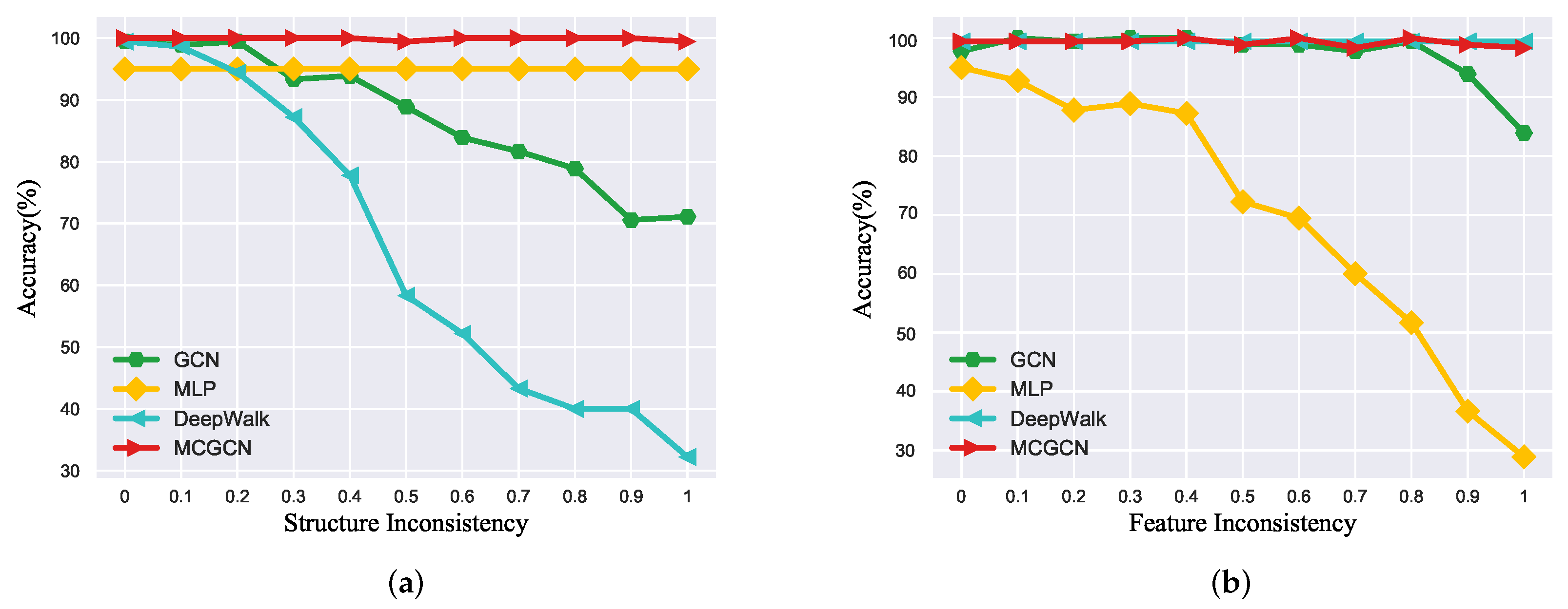
4.1. Setting One: Structure Inconsistency
4.2. Setting Two: Feature Inconsistency
4.3. Motivation
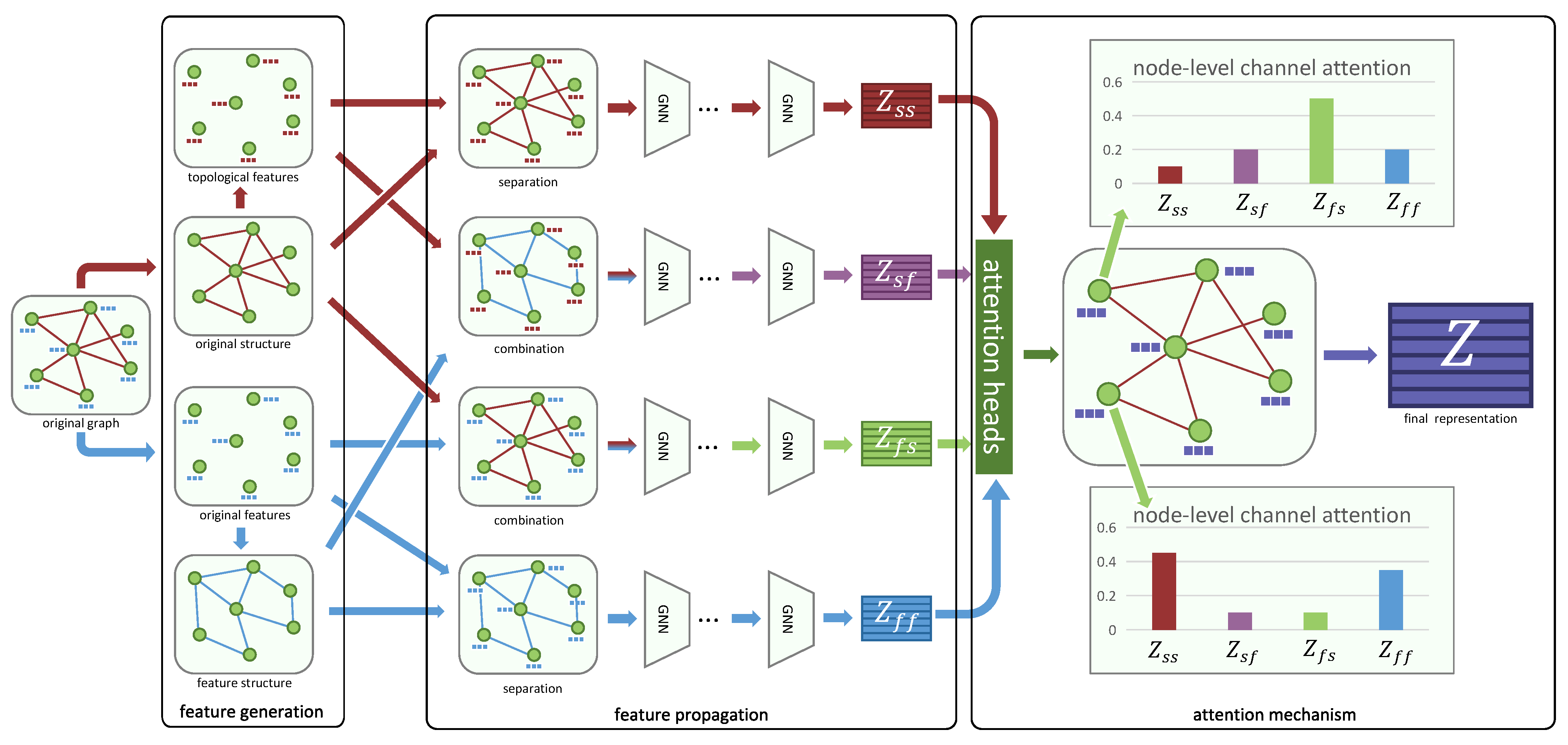
5. Methodology
5.1. Overview
5.2. Specific Convolution Channels
5.3. Joint Convolution Channels
5.4. Attention Mechanism
5.5. Optimization Objective
6. Experiments
6.1. Experimental Setting
6.1.1. Datasets
6.1.2. Baselines
6.1.3. Parameter Setting
6.2. Results and Analysis
6.2.1. Node Classification
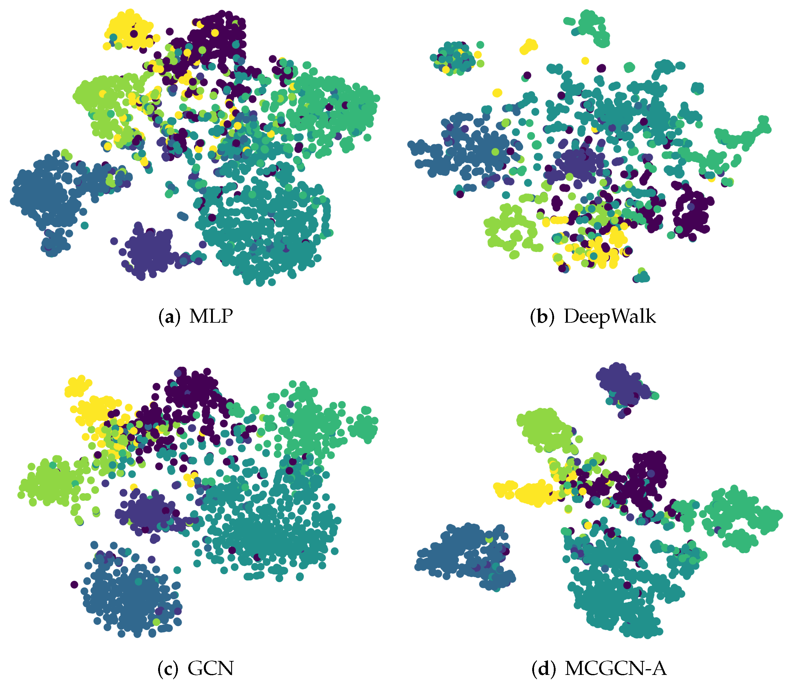
6.2.2. Visualization
6.2.3. Synthetic Experiments
6.2.4. Attention Analysis
6.3. Case Study on Recommendation Task
6.3.1. Datasets
6.3.2. Baselines
6.3.3. Metrics
6.3.4. Results and Analysis
7. Conclusions and Future Work
Author Contributions
Funding
Data Availability Statement
Conflicts of Interest
References
- Mitchell, J.C. Social networks. Annu. Rev. Anthropol. 1974, 3, 279–299. [Google Scholar] [CrossRef]
- Milroy, L.; Llamas, C. Social networks. In The Handbook of Language Variation and Change; Wiley-Blackwell: Oxford, UK, 2013; pp. 407–427. [Google Scholar]
- Radicchi, F.; Fortunato, S.; Vespignani, A. Citation networks. In Models of Science Dynamics: Encounters between Complexity Theory and Information Sciences; Springer: Berlin/Heidelberg, Germany, 2011; pp. 233–257. [Google Scholar]
- Greenberg, S.A. How citation distortions create unfounded authority: Analysis of a citation network. BMJ 2009, 339, b2680. [Google Scholar] [CrossRef] [PubMed]
- Shaw, M.E. Communication networks. In Advances in Experimental Social Psychology; Elsevier: Amsterdam, The Netherlands, 1964; Volume 1, pp. 111–147. [Google Scholar]
- Monge, P.R.; Contractor, N.S. Theories of Communication Networks; Oxford University Press: New York, NY, USA, 2003. [Google Scholar]
- Alm, E.; Arkin, A.P. Biological networks. Curr. Opin. Struct. Biol. 2003, 13, 193–202. [Google Scholar] [CrossRef] [PubMed]
- Girvan, M.; Newman, M.E. Community structure in social and biological networks. Proc. Natl. Acad. Sci. USA 2002, 99, 7821–7826. [Google Scholar] [CrossRef] [PubMed]
- Grover, A.; Leskovec, J. node2vec: Scalable feature learning for networks. In Proceedings of the 22nd ACM SIGKDD International Conference on Knowledge Discovery and Data Mining, San Francisco, CA, USA, 13–17 August 2016; pp. 855–864. [Google Scholar]
- Chen, Y.; Wu, L.; Zaki, M. Iterative deep graph learning for graph neural networks: Better and robust node embeddings. Adv. Neural Inf. Process. Syst. 2020, 33, 19314–19326. [Google Scholar]
- Kipf, T.N.; Welling, M. Semi-supervised classification with graph convolutional networks. In Proceedings of the ICLR, Toulon, France, 24–26 April 2017. [Google Scholar]
- Tang, J.; Aggarwal, C.C.; Liu, H. Node classification in signed social networks. In Proceedings of the ICDM, Barcelona, Spain, 12–15 December 2016; pp. 54–62. [Google Scholar]
- Gao, S.; Denoyer, L.; Gallinari, P. Temporal link prediction by integrating content and structure information. In Proceedings of the CIKM, Scotland, UK, 24–28 October 2011; pp. 1169–1174. [Google Scholar]
- Yu, X.; Han, J. Personalized entity recommendation: A heterogeneous information network approach. In Proceedings of the WSDM, New York City, NY, USA, 24–28 February 2014; pp. 283–292. [Google Scholar]
- Hamilton, W.L.; Ying, Z.; Leskovec, J. Inductive representation learning on large graphs. In Proceedings of the NIPS, Long Beach, CA, USA, 12–24 December 2017; pp. 1024–1034. [Google Scholar]
- Velickovic, P.; Cucurull, G.; Casanova, A.; Romero, A.; Liò, P.; Bengio, Y. Graph attention networks. In Proceedings of the ICLR, Vancouver, BC, Canada, 30 April–3 May 2018. [Google Scholar]
- Xu, K.; Hu, W.; Leskovec, J.; Jegelka, S. How Powerful are Graph Neural Networks? In Proceedings of the ICLR, New Orleans, LA, USA, 6–9 May 2019. [Google Scholar]
- Shervashidze, N.; Schweitzer, P.; van Leeuwen, E.J.; Mehlhorn, K.; Borgwardt, K.M. Weisfeiler-Lehman Graph Kernels. J. Mach. Learn. Res. 2011, 12, 2539–2561. [Google Scholar]
- Wu, F.; Souza, A.; Zhang, T.; Fifty, C.; Yu, T.; Weinberger, K. Simplifying Graph Convolutional Networks. In Proceedings of the ICML, Long Beach, CA, USA, 10–15 June 2019; pp. 6861–6871. [Google Scholar]
- Li, Q.; Han, Z.; Wu, X. Deeper Insights Into Graph Convolutional Networks for Semi-Supervised Learning. In Proceedings of the AAAI, New Orleans, LA, USA, 2–7 February 2018; pp. 3538–3545. [Google Scholar]
- Qin, M.; Jin, D.; Lei, K.; Gabrys, B.; Musial-Gabrys, K. Adaptive community detection incorporating topology and content in social networks. Knowl. Based Syst. 2018, 161, 342–356. [Google Scholar] [CrossRef]
- Zügner, D.; Akbarnejad, A.; Günnemann, S. Adversarial attacks on neural networks for graph data. In Proceedings of the 24th ACM SIGKDD International Conference on Knowledge Discovery & Data Mining, New York, NY, USA, 19–23 August 2018; pp. 2847–2856. [Google Scholar]
- Perozzi, B.; Al-Rfou, R.; Skiena, S. DeepWalk: Online learning of social representations. In Proceedings of the KDD, New York, NY, USA, 24–27 August 2014; pp. 701–710. [Google Scholar]
- Pal, S.K.; Mitra, S. Multilayer perceptron, fuzzy sets, and classification. IEEE Trans. Neural Netw. 1992, 3, 683–697. [Google Scholar] [CrossRef]
- Zhu, J.; Yan, Y.; Zhao, L.; Heimann, M.; Akoglu, L.; Koutra, D. Beyond Homophily in Graph Neural Networks: Current Limitations and Effective Designs. In Proceedings of the NIPS, Virtual-only Conference, 6–12 December 2020. [Google Scholar]
- Pei, H.; Wei, B.; Chang, K.C.; Lei, Y.; Yang, B. Geom-GCN: Geometric Graph Convolutional Networks. In Proceedings of the ICLR, Virtual-only Conference, 26 April–1 May 2020. [Google Scholar]
- Zhu, J.; Rossi, R.A.; Rao, A.B.; Mai, T.; Lipka, N.; Ahmed, N.K.; Koutra, D. Graph Neural Networks with Heterophily. In Proceedings of the AAAI, Virtual-only Conference, 2–9 February 2021. [Google Scholar]
- Yan, Y.; Hashemi, M.; Swersky, K.; Yang, Y.; Koutra, D. Two Sides of the Same Coin: Heterophily and Oversmoothing in Graph Convolutional Neural Networks. arXiv 2021, arXiv:2102.06462. [Google Scholar]
- Chien, E.; Peng, J.; Li, P.; Milenkovic, O. Adaptive Universal Generalized PageRank Graph Neural Network. In Proceedings of the ICLR, Virtual-only Conference, 3–7 May 2021. [Google Scholar]
- Wang, K.; Zhu, Y.; Liu, H.; Zang, T.; Wang, C. Learning Aspect-Aware High-Order Representations from Ratings and Reviews for Recommendation. ACM Trans. Knowl. Discov. Data 2023, 17, 1–22. [Google Scholar] [CrossRef]
- Guo, M.H.; Xu, T.X.; Liu, J.J.; Liu, Z.N.; Jiang, P.T.; Mu, T.J.; Zhang, S.H.; Martin, R.R.; Cheng, M.M.; Hu, S.M. Attention mechanisms in computer vision: A survey. Comput. Vis. Media 2022, 8, 331–368. [Google Scholar] [CrossRef]
- Niu, Z.; Zhong, G.; Yu, H. A review on the attention mechanism of deep learning. Neurocomputing 2021, 452, 48–62. [Google Scholar] [CrossRef]
- Scarselli, F.; Gori, M.; Tsoi, A.C.; Hagenbuchner, M.; Monfardini, G. The Graph Neural Network Model. IEEE Trans. Neural Netw. 2009, 20, 61–80. [Google Scholar] [CrossRef]
- Wu, Z.; Pan, S.; Chen, F.; Long, G.; Zhang, C.; Yu, P.S. A Comprehensive Survey on Graph Neural Networks. IEEE Trans. Neural Netw. Learn. Syst. 2021, 32, 4–24. [Google Scholar] [CrossRef]
- Defferrard, M.; Bresson, X.; Vandergheynst, P. Convolutional Neural Networks on Graphs with Fast Localized Spectral Filtering. In Proceedings of the NIPS, Barcelona, Spain, 5–10 December 2016; pp. 3837–3845. [Google Scholar]
- Shuman, D.I.; Narang, S.K.; Frossard, P.; Ortega, A.; Vandergheynst, P. The Emerging Field of Signal Processing on Graphs: Extending High-Dimensional Data Analysis to Networks and Other Irregular Domains. IEEE Signal Process. Mag. 2013, 30, 83–98. [Google Scholar] [CrossRef]
- Ge, L.; Li, S.; Wang, Y.; Chang, F.; Wu, K. Global spatial-temporal graph convolutional network for urban traffic speed prediction. Appl. Sci. 2020, 10, 1509. [Google Scholar] [CrossRef]
- Chen, Z.; Li, S.; Yang, B.; Li, Q.; Liu, H. Multi-scale spatial temporal graph convolutional network for skeleton-based action recognition. In Proceedings of the AAAI, Virtual-only Conference, 2–9 February 2021; Volume 35, pp. 1113–1122. [Google Scholar]
- Shan, X.; Cao, J.; Huo, S.; Chen, L.; Sarrigiannis, P.G.; Zhao, Y. Spatial–temporal graph convolutional network for Alzheimer classification based on brain functional connectivity imaging of electroencephalogram. Hum. Brain Mapp. 2022, 43, 5194–5209. [Google Scholar] [CrossRef]
- Veličković, P.; Cucurull, G.; Casanova, A.; Romero, A.; Lio, P.; Bengio, Y. Graph attention networks. arXiv 2017, arXiv:1710.10903. [Google Scholar]
- Rong, Y.; Huang, W.; Xu, T.; Huang, J. Dropedge: Towards deep graph convolutional networks on node classification. arXiv 2019, arXiv:1907.10903. [Google Scholar]
- Wang, X.; Zhu, M.; Bo, D.; Cui, P.; Shi, C.; Pei, J. Am-gcn: Adaptive multi-channel graph convolutional networks. In Proceedings of the 26th ACM SIGKDD International Conference on Knowledge Discovery & Data Mining, New York, NY, USA, 6–10 July 2020; pp. 1243–1253. [Google Scholar]
- Zhang, H.; Tian, Q.; Han, Y. Multi channel spectrum prediction algorithm based on GCN and LSTM. In Proceedings of the 2022 IEEE 96th Vehicular Technology Conference (VTC2022-Fall), London, UK, 26–29 September 2022; pp. 1–5. [Google Scholar]
- Zhai, R.; Zhang, L.; Wang, Y.; Song, Y.; Yu, J. A multi-channel attention graph convolutional neural network for node classification. J. Supercomput. 2023, 79, 3561–3579. [Google Scholar] [CrossRef]
- Hu, F.; Zhu, Y.; Wu, S.; Wang, L.; Tan, T. Hierarchical Graph Convolutional Networks for Semi-supervised Node Classification. In Proceedings of the IJCAI, Macao, China, 10–16 August 2019; pp. 4532–4539. [Google Scholar]
- Karrer, B.; Newman, M.E.J. Stochastic blockmodels and community structure in networks. Phys. Rev. 2010, 83, 016107. [Google Scholar] [CrossRef] [PubMed]
- Chen, X.; Chen, S.; Yao, J.; Zheng, H.; Zhang, Y.; Tsang, I.W. Learning on attribute-missing graphs. IEEE Trans. Pattern Anal. Mach. Intell. 2020, 44, 740–757. [Google Scholar] [CrossRef]
- Liu, W.; Wen, Y.; Yu, Z.; Yang, M. Large-margin softmax loss for convolutional neural networks. In Proceedings of the 33rd International Conference on International Conference on Machine Learning, New York, NY, USA, 19–24 June 2016; Volume 48, pp. 507–516. [Google Scholar]
- Tang, J.; Sun, J.; Wang, C.; Yang, Z. Social influence analysis in large-scale networks. In Proceedings of the KDD, Paris, France, 28 June–1 July 2009; pp. 807–816. [Google Scholar]
- Rozemberczki, B.; Allen, C.; Sarkar, R. Multi-Scale attributed node embedding. J. Complex Netw. 2021, 9, cnab014. [Google Scholar] [CrossRef]
- Sen, P.; Namata, G.; Bilgic, M.; Getoor, L.; Gallagher, B.; Eliassi-Rad, T. Collective Classification in Network Data. AI Mag. 2008, 29, 93–106. [Google Scholar] [CrossRef]
- Namata, G.M.; London, B.; Getoor, L.; Huang, B. Query-driven Active Surveying for Collective Classification. In Proceedings of the Workshop on Mining and Learning with Graphs (MLG), Edinburgh, UK, 1 July 2012. [Google Scholar]
- Hinton, G.E. Visualizing High-Dimensional Data Using t-SNE. Vigiliae Christ. 2008, 9, 2579–2605. [Google Scholar]
- Chang, X.; Wang, J.; Guo, R.; Wang, Y.; Li, W. Asymmetric Graph Contrastive Learning. Mathematics 2023, 11, 4505. [Google Scholar] [CrossRef]
- Yang, Z.; Yang, D.; Dyer, C.; He, X.; Smola, A.; Hovy, E. Hierarchical attention networks for document classification. In Proceedings of the 2016 Conference of the North American Chapter of the Association for Computational Linguistics: Human Language Technologies, San Diego, CA, USA, 12–17 June 2016; pp. 1480–1489. [Google Scholar]


| Dataset | Texas | Wisconsin | Cornell | Squirrel | Chameleon | Film | Cora | Citeseer |
|---|---|---|---|---|---|---|---|---|
| # Nodes | 183 | 251 | 183 | 5201 | 2277 | 7600 | 2708 | 3327 |
| #Edges | 309 | 499 | 295 | 217,073 | 36,101 | 33,544 | 5429 | 4732 |
| #Features | 1703 | 1703 | 1703 | 2089 | 2325 | 931 | 1433 | 3703 |
| #Classes | 5 | 5 | 5 | 5 | 5 | 5 | 7 | 6 |
| Texas | Wisconsin | Cornell | Squirrel | Chameleon | Film | Cora | Citeseer | |
|---|---|---|---|---|---|---|---|---|
| DeepWalk | 49.19 ± 0.38 | 53.51 ± 1.10 | 44.12 ± 0.52 | 32.37 ± 0.95 | 42.61 ± 0.42 | 23.74 ± 0.56 | 76.08 ± 0.63 | 53.59 ± 0.63 |
| MLP | 77.30 ± 0.55 | 83.01 ± 1.02 | 77.98 ± 0.83 | 34.39 ± 0.43 | 45.47 ± 0.37 | 32.78 ± 0.52 | 72.30 ± 0.88 | 70.17 ± 0.62 |
| GCN | 52.16 ± 1.04 | 55.88 ± 0.97 | 52.70 ± 0.71 | 37.96 ± 1.13 | 60.03 ± 0.74 | 27.92 ± 0.51 | 85.21 ± 0.53 | 73.68 ± 0.47 |
| GAT | 58.38 ± 0.48 | 54.41 ± 0.94 | 54.32 ± 0.38 | 30.03 ± 1.28 | 59.93 ± 0.69 | 28.15 ± 0.92 | 85.34 ± 0.73 | 73.92 ± 0.43 |
| H2GCN | 77.57 ± 0.87 | 81.72 ± 0.74 | 77.81 ± 0.69 | 40.14 ± 0.47 | 59.64 ± 1.02 | 31.63 ± 0.49 | 85.27 ± 0.32 | 74.42 ± 0.49 |
| GPRGNN | 77.83 ± 0.43 | 81.96 ± 0.96 | 77.93 ± 0.98 | 41.81 ± 0.89 | 60.09 ± 0.73 | 33.25 ± 0.47 | 85.79 ± 0.36 | 73.37 ± 0.90 |
| MCGCN-A | 78.46 ± 0.39 | 82.39 ± 0.91 | 78.65 ± 0.59 | 41.74 ± 1.28 | 59.91 ± 0.47 | 33.46 ± 0.62 | 86.32 ± 0.60 | 74.04 ± 0.67 |
| MCGCN-I | 78.39 ± 0.47 | 82.55 ± 0.42 | 78.21 ± 0.38 | 42.21 ± 1.79 | 61.64 ± 0.35 | 33.17 ± 0.58 | 86.28 ± 0.74 | 74.51 ± 0.34 |
| #Person | #Job | #Interaction | #Recommend | #Interview | #Offer |
|---|---|---|---|---|---|
| 9719 | 2035 | 15,101 | 1735 | 952 | 159 |
| Method | AUC | Accuracy | Recall | F1 Score |
|---|---|---|---|---|
| GCN | 0.7789 | 0.7347 | 0.9155 | 0.7753 |
| GAT | 0.8176 | 0.7300 | 0.9765 | 0.7834 |
| AGC | 0.8909 | 0.6596 | 0.9437 | 0.7349 |
| HAN | 0.6465 | 0.5266 | 0.7230 | 0.5693 |
| Ours | 0.8448 | 0.7483 | 0.9395 |
Disclaimer/Publisher’s Note: The statements, opinions and data contained in all publications are solely those of the individual author(s) and contributor(s) and not of MDPI and/or the editor(s). MDPI and/or the editor(s) disclaim responsibility for any injury to people or property resulting from any ideas, methods, instructions or products referred to in the content. |
© 2024 by the authors. Licensee MDPI, Basel, Switzerland. This article is an open access article distributed under the terms and conditions of the Creative Commons Attribution (CC BY) license (https://creativecommons.org/licenses/by/4.0/).
Share and Cite
Chang, X.; Wang, J.; Wang, R.; Wang, T.; Wang, Y.; Li, W. Multi-Channel Graph Convolutional Networks for Graphs with Inconsistent Structures and Features. Electronics 2024, 13, 607. https://doi.org/10.3390/electronics13030607
Chang X, Wang J, Wang R, Wang T, Wang Y, Li W. Multi-Channel Graph Convolutional Networks for Graphs with Inconsistent Structures and Features. Electronics. 2024; 13(3):607. https://doi.org/10.3390/electronics13030607
Chicago/Turabian StyleChang, Xinglong, Jianrong Wang, Rui Wang, Tao Wang, Yingkui Wang, and Weihao Li. 2024. "Multi-Channel Graph Convolutional Networks for Graphs with Inconsistent Structures and Features" Electronics 13, no. 3: 607. https://doi.org/10.3390/electronics13030607
APA StyleChang, X., Wang, J., Wang, R., Wang, T., Wang, Y., & Li, W. (2024). Multi-Channel Graph Convolutional Networks for Graphs with Inconsistent Structures and Features. Electronics, 13(3), 607. https://doi.org/10.3390/electronics13030607