Incremental Scene Classification Using Dual Knowledge Distillation and Classifier Discrepancy on Natural and Remote Sensing Images

Abstract

Conventional deep neural networks face challenges in handling the increasing amount of information in real-world scenarios where it is impractical to gather all the training data at once. Incremental learning, also known as continual learning, provides a solution for lightweight and sustainable learning with neural networks. However, incremental learning encounters issues such as “catastrophic forgetting” and the “stability–plasticity dilemma”. To address these challenges, this study proposes a two-stage training method. In the first stage, dual knowledge distillation is introduced, including feature map-based and response-based knowledge distillation. This approach prevents the model from excessively favoring new tasks during training, thus addressing catastrophic forgetting. In the second stage, an out-of-distribution dataset is incorporated to calculate the discrepancy loss between multiple classifiers. By maximizing the discrepancy loss and minimizing the cross-entropy loss, the model improves the classification accuracy of new tasks. The proposed method is evaluated using the CIFAR100 and RESISC45 benchmark datasets, comparing it to existing approaches. Experimental results demonstrate an overall accuracy improvement of 6.9% and a reduction of 5.1% in the forgetting rate after adding nine consecutive tasks. These findings indicate that the proposed method effectively mitigates catastrophic forgetting and provides a viable solution for image classification in natural and remote sensing images.

1. Introduction

The advancements in hardware devices and the availability of vast amounts of data have led to improved performance of machine learning techniques across various domains, particularly deep learning. Deep learning has gained significant attention in the academic community. By automatically learning features from a huge amount of data, deep learning reduces the need for independent feature extraction, not only reducing human effort but also enhancing the accuracy and robustness of classification. As a result, research in the field of deep learning has experienced significant growth in recent years, particularly in computer vision [1].

Typically, a deep learning model necessitates an adequate amount of data in each category during training to achieve desirable outcomes. However, real-world data are often dynamic and ever-evolving. As the data volume increases, training a neural network model with the entire dataset becomes computationally intensive and time-consuming, posing challenges in effectively handling such scenarios. If only new data are utilized to update the model, the model may suffer from the issue of forgetting previously acquired knowledge, leading to a decline in performance. This phenomenon is commonly known as “catastrophic forgetting” [2]. As a potential solution to this problem, the concept of incremental learning has emerged.

Incremental learning, also known as lifelong learning or continuous learning, is a deep learning technique aimed at enabling models to effectively process and integrate new information while retaining existing knowledge, mirroring the natural learning process observed in humans. Compared to traditional machine learning approaches, incremental learning offers several advantages. It allows for training with new data at any time, with or without the inclusion of old data, and enables continuous learning based on existing models without the need for complete retraining, resulting in reduced time and computational costs. This approach enhances the model’s ability to adapt to evolving data, ensuring high efficiency and accuracy in dynamic environments, thus closely resembling the learning patterns observed in humans.

The challenge of catastrophic forgetting remains a significant obstacle in incremental learning. Some approaches have explored the utilization of a limited number of samples from old tasks stored in a memory bank to mitigate catastrophic forgetting. However, it should be noted that the loss of the old task dataset or privacy concerns may hinder the successful implementation of these approaches. Another challenge in the context of incremental learning pertains to maintaining the adaptability and accuracy of the model, a phenomenon commonly referred to as the “stability–plasticity dilemma”. The concept of stability in this context relates to the model’s ability to retain the knowledge acquired from previous tasks, while plasticity refers to its capacity to integrate new knowledge effectively. Just as humans face this dilemma when acquiring new knowledge, striking a balance between assimilating new tasks and preserving the essence of previously learned tasks becomes crucial. Finding the equilibrium within this complicated situation presents a significant challenge in the field of incremental learning.

Deep neural networks have demonstrated remarkable performance in the field of computer vision, which has motivated researchers to explore their application in addressing challenges associated with remote sensing images [3,4]. The processing of remote sensing images involves handling large volumes of data, which is a computationally intensive task. Furthermore, certain remote sensing images may contain sensitive data that could potentially become inaccessible over time. Therefore, incremental learning is an alternative approach that continuously adds new data samples to update deep neural networks, gradually learning new knowledge without retraining the entire network.

It is important to note that this study concentrates on class incremental learning (class-IL), which involves evaluating all the categories learned by the model after each batch of learning tasks. Moreover, this study considers the most challenging scenario, where training data from past or future tasks cannot be utilized during the training of the current task. This limitation often leads to significant catastrophic forgetting during training, resulting in a decline in performance for previously learned tasks. To address this, this study adopts an approach of training the model using an auxiliary dataset and investigates whether it can effectively strike a balance between the “stability–plasticity dilemma”.

This study presents the following contributions:

• A novel two-stage incremental learning method is proposed, leveraging a regularization approach. The method incorporates a dual distillation process, which includes feature map knowledge distillation and response-based knowledge distillation. The feature map knowledge distillation process ensures that the model’s feature extraction process remains balanced and not solely influenced by the new task data. Since the feature extractors were altered, the response-based knowledge distillation is employed to address the challenge of catastrophic forgetting and mitigate its risks.
• This study employs the calculation of discrepancy loss between multiple classifiers, achieved through training on out-of-distribution datasets. This approach brings the decision boundary of the new task model closer to the data distribution of the new task categories, eventually enhancing the classification performance of the new task.
• The feasibility of applying incremental learning methods from natural image classification problems to remote sensing image classification problems is explored, expanding the potential applications of incremental learning in different domains.

The rest of this paper is organized as follows. Section 2 provides a brief introduction to the domain of incremental learning and reviews some previous studies. The proposed method is described in Section 3, followed by the experiments and discussions in Section 4. Lastly, Section 5 proposes future research directions to further advance incremental learning in practical applications.

2. Literature Review

This section presents an overview of incremental learning problems, approaches, and their limitations through a review of several previous studies. Firstly, the scenarios of incremental learning are introduced. Then, the different types of approaches used to address these problems are discussed, along with a description of the challenges they encounter.

2.1. Scenarios of Incremental Learning

To assess a model’s ability for incremental learning, van de Ven et al. [5] proposed three incremental learning scenarios: task-incremental learning (Task-IL), domain-incremental learning (Domain-IL), and class-incremental learning (Class-IL).

In Task-IL, the algorithm gradually learns different tasks. During testing, the algorithm is aware of the specific task it should perform. The model architecture may incorporate task-specific components, such as independent output layers or separate networks, while sharing other parts of the network, such as weights or loss functions, across tasks. Task-IL aims to prevent catastrophic forgetting and explore effective ways to share learned features, optimize efficiency, and leverage information from one task to improve performance in other tasks. This scenario can be compared to learning different sports.

Domain-IL involves a consistent task problem structure with continuously changing input distributions. During testing, the model does not need to infer the task it belongs to but rather focuses on solving the current task at hand. Preventing catastrophic forgetting in Domain-IL remains challenging, and addressing this issue is an important unsolved challenge. An analogy in the real world is adapting to different protocols or driving in various weather conditions [6].

Class-IL requires the model to infer the task it is facing during testing and solve all previously trained tasks. After a series of classification tasks, the model must learn to distinguish all classes. The key challenge in Class-IL lies in effectively learning to differentiate previous classes that have not been observed together in the current task, which poses a significant challenge for deep neural networks [7,8].

2.2. Approaches of Incremental Learning

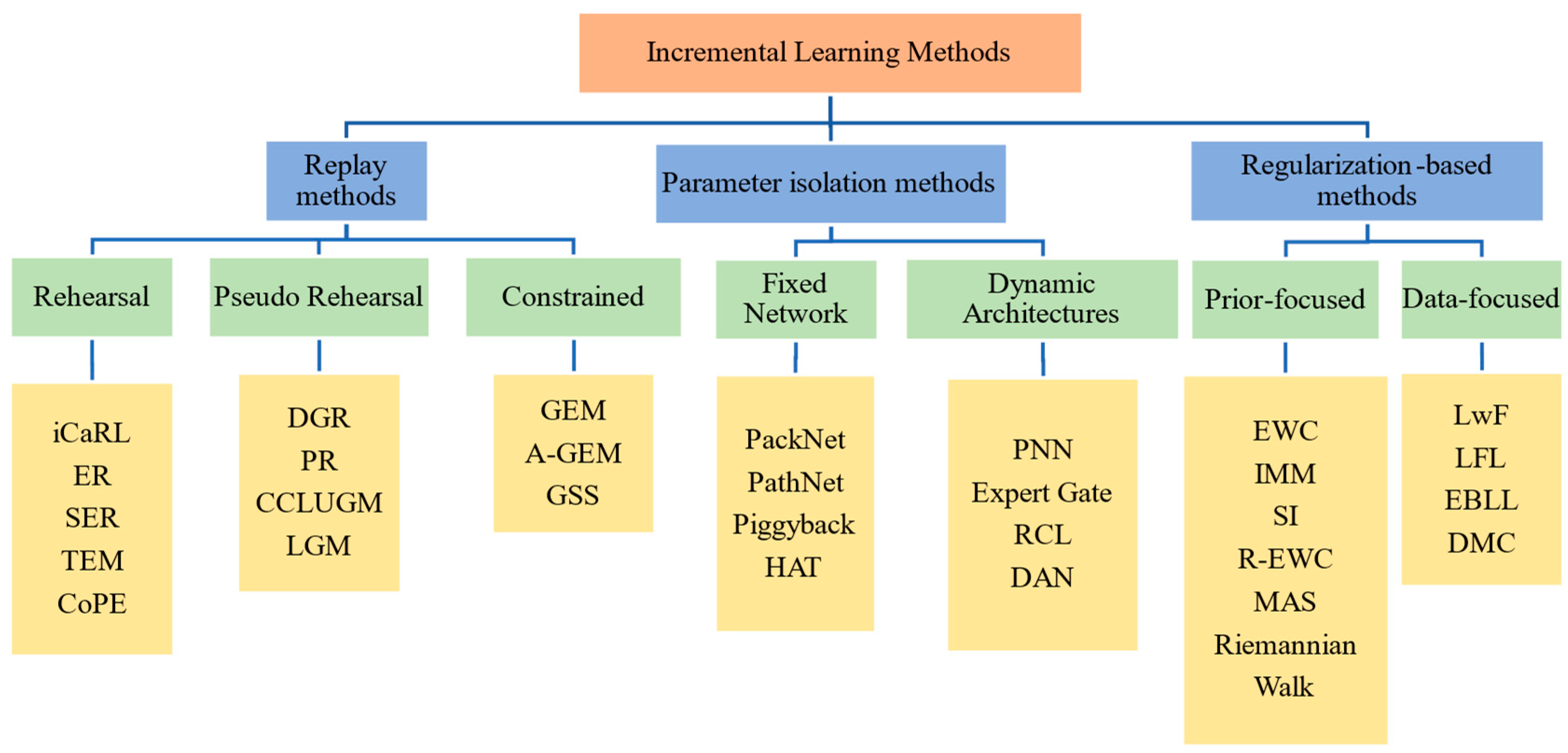
In this study, following the research of De Lange et al. [9], the methods for implementing incremental learning are categorized into three main categories: replay methods, parameter isolation methods, and regularization-based methods. Figure 1 illustrates a tree-structured diagram of different incremental learning methods. A brief overview of some of these methods is provided below.

Replay methods involve storing samples in their original format or generating virtual samples (pseudo-data) using generative models. These samples from previous tasks are included in the training process to reduce forgetting. Replay methods can be further divided into two strategies. The first strategy is Rehearsal/Pseudo-Rehearsal, which retains a subset of representative samples from previous tasks and utilizes them during the training of new tasks. Representative learning methods, such as iCaRL [10], fall under this category.

To address concerns related to data privacy leakage and overfitting to retain old data, a variation of replay methods called Pseudo-Rehearsal is employed when previous samples are not available. This strategy involves inputting random numbers into a trained model to generate virtual samples that approximate the original sample data. DGR [11], for example, trains a deep generative model “generator” in the framework of generative adversarial networks to generate data similar to past data. However, it should be noted that the results of using the Pseudo-Rehearsal method are generally not as effective as the Rehearsal strategy. Another strategy known as Constrained Optimization restricts the optimization of the new task loss function to prevent interference from old tasks. GEM [12] is a representative algorithm that adopts this approach.

Parameter isolation methods aim to prevent forgetting by allocating different parameters for each task. Some methods within this category involve adding new branches for new tasks while freezing the parameters of old tasks [13] or providing dedicated model copies for each task [14] when the model architecture allows. For parameter isolation methods that maintain a static model architecture, specific portions are allocated to each task. During the training of a new task, the portions associated with previous tasks are masked to prevent parameter updates, thereby preserving the knowledge acquired from previous tasks. Representative methods include the PathNet [15], PackNet [16], and HAT [17].

Regularization-based methods introduce an additional regularization term in the loss function to consolidate previous knowledge when learning new data. These methods prioritize data privacy, reduce memory requirements, and avoid the use of old data for training. Examples of regularization-based methods include Learning without Forgetting (LwF) [18] and Elastic Weight Consolidation (EWC) [19]. LwF leverages the output distribution of the old model as knowledge and transfers it to the training of the new model. EWC calculates the importance of all neural network parameters to limit the degree of change in important parameters.

Among the three methods, the Rehearsal strategy (iCaRL) often outperforms the other two types of methods. This is because the Rehearsal strategy allows for the direct involvement of old data in training, resulting in improved performance. However, it does not fully meet the extreme situation of incremental learning, which demands the exclusion of old data. On the other hand, methods employing the Pseudo-Rehearsal strategy rely heavily on the quality of the generated samples. The overall learning outcomes are significantly compromised and even perform worse than the other two methods with a poor generator.

Although regularization-based methods avoid the use of old data, which aligns more closely with the real-world scenario that incremental learning aims to simulate, they are often vulnerable to domain changes between tasks, particularly when the domains differ significantly. This leads to the persistent problem of catastrophic forgetting. Consequently, many regularization-based methods employ knowledge distillation to retain knowledge from old tasks as much as possible to mitigate the issue of catastrophic forgetting, which will be reviewed in the next subsection.

2.3. Knowledge Distillation

To retain the knowledge of previous tasks, regularization-based methods often employ the technique of knowledge distillation (KD). Knowledge distillation is a model compression technique that effectively extracts knowledge from a more complex neural network model to produce a smaller and simpler model that can perform on par with the complex model. This technique has been widely utilized not only in incremental learning but also in various other fields, such as computer vision, natural language processing, speech recognition, and recommendation systems.

The concept of using knowledge distillation to compress models was first introduced by Bucilua et al. [20] in 2006, although no practical implementation was provided. In 2014, Hinton et al. [21] formally defined the term “distillation” and proposed a practical training process. The process involves a teacher–student model framework, where the teacher model is initially trained and then distilled to extract knowledge as teaching materials. This allows the student model to achieve performance comparable to the teacher model. Specifically, the teacher model can be an initial or trained model, while the student model is the model that needs to undergo training. The final output of the entire framework is based on the results obtained from training the student model.

In knowledge distillation, the architecture of the teacher–student relationship serves as a general carrier for knowledge transfer. The quality of knowledge acquisition and distillation from teacher to student is determined by the design of the teacher and student networks. Similar to human learning, students need to find suitable teachers from whom to learn. Therefore, in knowledge distillation, factors such as the type of knowledge, distillation strategy, and the structural relationship between the teacher and student models significantly impact the learning process of the student model. Most knowledge distillation methods utilize the output of a large deep model as knowledge [22,23,24]. Alternatively, some methods employ the activation functions or feature neurons of intermediate layers as knowledge [25,26,27,28].

In a survey conducted by Gou et al. [29], the authors categorized knowledge in knowledge distillation into three types: response-based knowledge, feature-based knowledge, and relation-based knowledge.

Response-based knowledge refers to the output of neurons in the last layer of the teacher model. The aim is to imitate the final predictions of the teacher model. This type of knowledge distillation is widely used in various tasks and applications, such as object detection [30] and semantic landmark localization. However, it has the limitation of relying solely on the output of the last layer, disregarding potential knowledge in hidden layers. Additionally, response-based knowledge distillation is primarily applicable to supervised learning problems.

Feature-based knowledge overcomes the limitation of neglecting hidden layers. In addition to the last layer output, intermediate layers’ output, specifically feature maps, can be utilized to improve the performance of the student model. For example, the Fitnets introduced by Romero et al. [31] adopted such an idea. Inspired by them, other methods have been proposed to match features during the distillation process indirectly [32,33,34]. While feature-based knowledge distillation provides valuable information for student model learning, challenges remain in selecting appropriate layers from the teacher and student models to match the feature representations effectively.

Relation-based knowledge explores relationships between different layers or different data samples, going beyond the specific layer outputs used in response-based and feature-based knowledge. For instance, Liu et al. [35] proposed a method that employs an instance relationship graph, where the knowledge transferred includes instance features, instance relationships, and feature space transformations across layers.

2.4. Out-of-Distribution Dataset

In the domain of computer vision, numerous studies have extensively explored the incorporation of external datasets to enhance the performance of target tasks. For instance, inductive transfer learning has been employed to transfer and reuse knowledge from labeled out-of-domain samples through external datasets [36,37]. Semisupervised learning approaches [38,39] aim to leverage the utility of unlabeled samples within the same domain, while the self-taught learning approach improves the performance of specific classification tasks using easily obtainable unlabeled data [40].

In a study by Yu et al. [41], auxiliary datasets were applied to unsupervised anomaly detection. The auxiliary dataset consists of unlabeled data, encompassing samples from known categories (referred to as in-distribution or ID samples) as well as datasets that deviate from the target task distribution (known as out-of-distribution (OOD) samples). OOD samples exhibit lower confidence levels, indicating their proximity to the classifier’s decision boundary. These samples are distinguished by analyzing the discrepancies between classifiers. Since OOD samples are not explicitly assigned to ID sample categories or lie far from the ID sample distribution, classifiers with varying parameters become perplexed and produce divergent outcomes. Consequently, OOD samples occupy the “gap” between the decision boundaries, thus enhancing the classifier’s classification performance on ID samples and facilitating the detection of OOD samples.

This study adopts a perspective similar to that of the investigation conducted by Yu et al. [41] in utilizing unlabeled auxiliary data. Based on our intuition, the auxiliary dataset should possess distinguishable characteristics that are distinct from the samples in the current task. When learning a new task, the objective is to identify the disparities between the current task and previous tasks. By incorporating classifier discrepancy with OOD data, the classification performance can be enhanced in scenarios where no data from previous tasks were utilized, as OOD data can serve as dissimilar data to the current task data.

2.5. Summary

After reviewing existing literature on incremental learning, this study focuses on exploring class-IL problems. Replay methods are often used but do not meet the challenging requirement of learning without old data. Parameter isolation methods are limited to Task-IL scenarios. Therefore, this study adopts a regularization-based approach and proposes a novel method that combines response-based and feature-based knowledge distillation. In addition, multiple classifiers and auxiliary datasets are introduced to enhance the classification performance of new tasks and strike a balance between stability and plasticity.

3. Methodology

In this section, we present the proposed two-stage incremental learning method.

3.1. Problem Definition

Assuming there are T tasks, $D_t=\left\{x_t,y_t\right\}, t=1,\dots ,T$ is developed, where $D_t$ represents the dataset of task t, and $x_t$ and $y_t$ are the samples and corresponding labels in task t. Each task t consists of distinct classes $C_t$, and the classes vary across tasks. In the context of Class-IL, the objective is to sequentially train the model from $D_1$ to $D_T$. As the number of tasks increases, the model gradually adapts to all the learned tasks, and the number of classes that the model needs to classify also grows. Specifically, when training task t, the model is trained exclusively on the dataset $D_t$. After training, the model should not only be capable of classifying the current task t but also retain the ability to classify the datasets $D_{1:t-1}$ from previously trained tasks. Therefore, the desired outcome is that after learning all tasks, the model can classify all observed datasets $D_{1:T}$ without experiencing any forgetting.

3.2. System Architecture

To achieve the objective stated in Section 3.1, this study introduces a two-stage training model for Class-IL. The model consists of a dual-headed CNN architecture that includes a shared feature extractor and two classifiers. Due to the different initialized parameters, the decision boundaries of these two classifiers may show slight variations after training.

First, the model learns based on an initial task dataset, $D_0$. The feature extractor of the model in this situation is called $F_0$, and the classifiers are called $C_0^{\left(1\right)}$ and $C_0^{\left(2\right)}$. After training, when training a new task, t, with dataset $D_t$, we divide the training process into two stages.

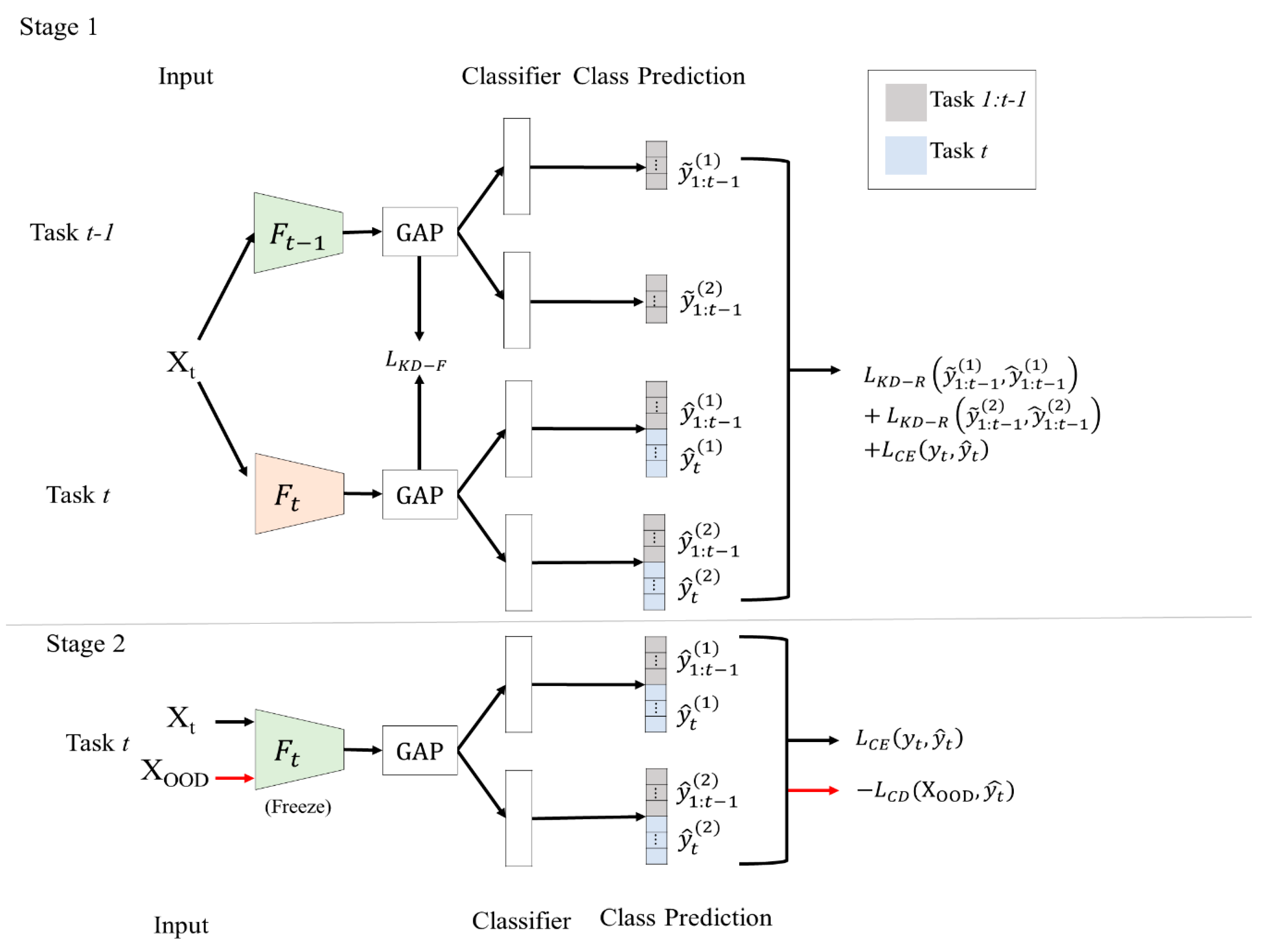
In the first stage, the output of $F_{t-1}$, ${\tilde{y}}_{1:t-1}^{\left(1\right)}$, and ${\tilde{y}}_{1:t-1}^{\left(2\right)}$ is considered as the knowledge of the old model. This knowledge is used to update the feature extractor, $F_t$, and the classifiers, $C_t^1$ and $C_t^2$, for task t. We calculate two distillation losses: the feature map distillation loss (called KD-F), which uses the outputs of $F_{t-1}$ and $F_t$, and the response distillation losses (called KD-R), which use the output logits ${\tilde{y}}_{1:t-1}^{\left(1\right)}$, and ${\tilde{y}}_{1:t-1}^{\left(2\right)}$ of the old tasks. Additionally, we calculate the cross-entropy loss of $D_t$ in the output logits of the new task to update the entire model.

The reason for using dual distillation loss is to ensure that the updated model in the training process of the new task can retain the feature extraction ability that is similar to the old model. It is important to note that since there is no old task data involved in learning a new task, we use the logits of the old task to calculate the response distillation loss. This is executed in the hope that during the training process of the new task, the updated model’s logits output can closely match the old model’s output, so that similar classification results on old tasks can be expected.

The first stage of the proposed method constrains the model with dual distillation loss, which may lead to an overreliance on recognizing the old task and a loss of the ability to learn new tasks. To address this issue, a second stage is introduced. In this stage, the discrepancy loss between the classifiers using auxiliary data is calculated to enhance the classification ability for new tasks. The goal of the classifier discrepancy loss is to increase the disparity between the two classifiers, while the cross-entropy loss reduces the discrepancy. Through the interplay between these two types of losses, the aim is to find the optimal decision boundary. The overall architecture is illustrated in Figure 2.

3.3. Dual Knowledge Distillation

In the study by Hinton et al. [21], they referred to knowledge based on responses as “soft targets”. “Soft targets” represent the probability that an input belongs to a certain class and can be estimated using the softmax function, as shown in Equations (1) and (2):

$$y\left({\mathrm{z}}_{\mathrm{i}},\tau \right)=\frac{exp\left(z_i/\tau \right)}{{\sum }_{j}exp\left(z_j/\tau \right)}$$

(1)

and

$${\mathcal{L}}_{KD}\left(y\left(z_t,\tau \right),y\left(z_s,\tau \right)\right)={\mathcal{L}}_R\left(y\left(z_t,\tau \right),y\left(z_s,\tau \right)\right)$$

(2)

where ${\mathcal{L}}_R$ represents the divergence loss of the logits, and $z_t$ and $z_s$ represent the logits output of the teacher and student models. Following the suggestion by Hinton et al. [21], a temperature $\tau$ should be set to a number larger than 1 to increase the weight of smaller logits, encouraging similarity between the teacher and student networks.

In this study, the knowledge distillation process is referred to as a self-distillation process, as the teacher and student networks are identical. The only difference lies in the training dataset used for different tasks. Thus, the objective of the knowledge distillation process is to obtain knowledge from the network itself, essentially learning from previous tasks.

The response-based knowledge distillation method involves variations in the extracted features of the network due to the incremented tasks, which can lead to challenges in adaptability and stability when learning different tasks or domains. This may result in catastrophic forgetting or ineffective learning of new tasks. In contrast, the feature-based knowledge distillation method relies solely on the feature representation of the model’s intermediate layer for knowledge transfer without depending on labeled prediction responses. It focuses on extracting and transferring the feature representations within the model, providing flexibility and adaptability to different tasks. However, relying solely on the feature-based knowledge distillation method can fail the classifier because the classifier does not reflect the change in the feature space. To address this issue, this study adopts a dual distillation approach, combining feature map distillation (KD-F) with the traditional knowledge distillation method based on logit outputs (KD-R). This approach enables the new model to not only learn the output results of the old model but also approximate the feature extraction results of the old model. Consequently, catastrophic forgetting is effectively mitigated while preserving the network’s ability to learn new tasks.

The feature map distillation loss is the mean square error (MSE) loss:

$$L_{KD-F}=\left|\left|F_{1:t-1}\left(X_t\right)-F_t\left(X_t\right)\right|\right|,$$

(3)

where $F_{1:t-1}\left(X_t\right)$ and $F_t\left(X_t\right)$ represent the output of the feature extraction layer of the new model and old model, respectively, at a specific training task t. During the training of a new task t, only the data $X_t$ from that task are used. Therefore, it is reasonable to expect that the feature vectors extracted using the new model should be similar to those extracted through the old model when facing “unseen” data that the old model has never encountered.

After applying feature map distillation, the model effectively approximates the feature distribution of the old model while learning the new task. However, including the categories of the previous task in the calculation of cross-entropy loss when training the new task, which uses only new task data, can lead to significant catastrophic forgetting. This is due to the tendency of the softmax function to bias the overall logit output towards the categories of the new task. As mentioned above, with the change in feature extraction results, the classifier for the previous task cannot ensure good discriminative ability in the new feature space. Hence, this study utilizes response-based logit output as a second knowledge distillation loss to reinforce the model’s classifier in preserving its classification capability for the categories of the previous task in the modified feature space. The equation for KD-R is presented in Equation (4):

$$L_{KD-R}\left({\tilde{y}}_{1:t-1}^{\left(k\right)},{\widehat{y}}_{1:t-1}^{\left(k\right)}\right)=-{\sum }_{i=1:t-1}{\tilde{y}}_{{\mathcal{l}}_i}^{\prime \left(k\right)}·log{\widehat{y}}_{{\mathcal{l}}_i}^{\prime \left(k\right)},$$

(4)

where ${\tilde{y}}_{1:t-1}^{\left(k\right)}$ is the logits of the old model, and ${\widehat{y}}_{1:t-1}^{\left(k\right)}$ is the logits of the kth classifier on old tasks’ categories. $\mathcal{l}$ is the categories from task 1 to t−1, ${\tilde{y}}_{{\mathcal{l}}_i}^{\prime \left(k\right)}$ is the soft target, and ${\widehat{y}}_{{\mathcal{l}}_i}^{\prime \left(k\right)}$ is the predicted output of the ith category from the new model.

In addition to the distillation loss, the cross-entropy loss is computed based on the predicted results of both classifiers (see Equation (5)). It is important to note that since only the data from the new task are used during the training of the new task, considering the categories of the old task when calculating the cross-entropy loss would result in significant forgetting. Therefore, in this study, the cross-entropy loss calculation only considers the output results of the new task categories. In other words, only the classifier for the categories of the new task is updated using the cross-entropy loss. The overall loss function is expressed using Equation (6):

$$L_{CE}=-\left(y_t^{\left(1\right)}·log{\widehat{y}}_t^{\left(1\right)}+y_t^{\left(2\right)}·log{\widehat{y}}_t^{\left(2\right)}\right)$$

(5)

and

$$L_{{stage}_I}=L_{CE}+\alpha {(L}_{KD-F}+L_{KD-R}),$$

(6)

where α is a weight factor. A higher α value leads to better performance in classifying old tasks.

3.4. Classifier Discrepancy Learning

This study is inspired by the work of Yu and Aizawa [41] and Saito et al. [42], which proposed the use of multiple classifiers and the simultaneous calculation of cross-entropy and classifier discrepancy loss to effectively enhance the classification performance of the classifiers during the learning process. The underlying concept of their approach is to enable each classifier to utilize different features for classification, thereby enhancing the model’s capability to classify diverse categories. By leveraging different classifiers, the model can capture distinct crucial information, leading to more stable classification results.

Since the information regarding the previous task is insufficient during the incremental learning process, there is no guarantee that the model will not cover the data distribution of the old task when solely relying on the training data of the new task. To address this concern, this study proposes the incorporation of an additional OOD dataset as auxiliary data. The goal is to utilize the OOD dataset with the discrepancy loss to create a separation between the two classifiers. For k classifiers, the classifier discrepancy loss is defined as follows:

$$L_{CD}\left(X_{OOD},{\widehat{y}}_t\right)={\sum }_{m=1}^k{\sum }_{n=m+1}^{k}d\left(p_m\left(y_t|X_{OOD}\right),p_n\left(y_t|X_{OOD}\right)\right),$$

(7)

where the discrepancy loss for a single classifier is defined as follows:

$$\mathrm{d}\left(p_m\left(y_t|X_{OOD}\right),p_n\left(y_t|X_{OOD}\right)\right)=\left|p_m\left({\widehat{y}}_t|X_{OOD}\right)\mathrm{ }-\mathrm{ }{p}_n\left({\widehat{y}}_t|X_{OOD}\right)\right|.$$

(8)

In this study, k is set to 2 because there is no significant performance difference when using more classifiers, as described in [42].

Simultaneously, the optimization of the two classifiers is continuously performed using the cross-entropy loss. This approach enables better convergence of the decision boundary of the model. The overall loss function in stage II is shown in Equation (9):

$$L_{stag{e}_{II}}=\mathrm{ }{L}_{CE}\mathrm{ }-\mathrm{ }\lambda L_{CD},$$

(9)

where the computation of $L_{CE}$ is the same as that in stage I. The weight λ represents the balance between the discrepancy loss of the classifier and the cross-entropy loss. When λ is too small, for example, λ = 0.5, it cannot effectively separate the decision boundaries between two classifiers, resulting in a bias towards learning the new tasks by strongly minimizing the cross-entropy loss in the second stage. Therefore, there may be overfitting of the new tasks in subsequent tasks. On the other hand, when λ is too large, for example, λ = 2, the decision boundaries between the classifiers may be too widely separated, resulting in more noticeable differences between the classifiers. Therefore, after experimentation, we chose λ = 1 for successive experiments. It is important to note that in the second stage, we freeze the well-trained feature extractor $F_t$ for the model to focus on improving the classifiers.

In the next section, we will introduce the experimental results of this study. We will also discuss the performance of the proposed method on both natural image and remote sensing image datasets.

4. Results and Discussions

In this section, several experiments and discussions are conducted to demonstrate the validity of the proposed approach.

4.1. Datasets and Experimental Settings

This study explores the feasibility of the proposed framework using two types of datasets. The first dataset used is CIFAR100 [43], a natural image dataset, while the corresponding auxiliary dataset is Tiny Imagenet [44]. The auxiliary dataset, Tiny Imagenet, is employed in the second stage of training and is considered unlabeled. For the experiment, CIFAR100 is divided into ten tasks, each consisting of ten classes. The initial task comprises a set of 10 classes. In the first incremented task, an additional 10 classes are introduced, resulting in the model being required to classify a total of 20 classes using only the training samples from the newly added 10 classes. This process continues until the ninth incremented task is reached, at which point the model must classify all 100 classes.

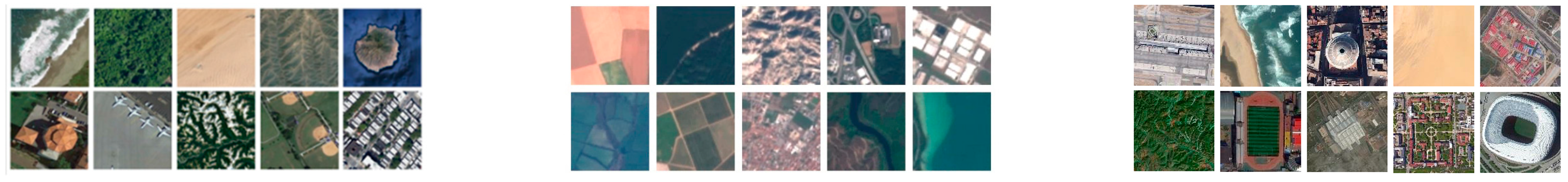
Additionally, remote sensing image datasets, namely NWPU-RESISC45 [45], UC-Merced [46], and AID [47], are used. These benchmark datasets are widely utilized to assess the performance of the model and demonstrate the general applicability in the domain of remote sensing imagery. NWPU-RESISC45 contains 31,500 images, covering 45 scene classes with 700 images per class. Each image has a size of 256 × 256 pixels, but for the experiment, the images are resized to 64 × 64 pixels. AID comprises 10,000 images divided into 30 classes, with each image measuring 600 × 600 pixels. UC-Merced consists of 21 classes with 100 images per class. Some sample images are shown in Figure 3. In the experiments involving the remote sensing image dataset, the RESISC45 is used as the training dataset, while the others are combined to create the auxiliary dataset.

Due to the limitation of the number of samples in the RESISC45 remote sensing dataset, the training dataset is divided into five tasks (nine classes for each task), and the images are resized to 64 × 64 pixels. Each class is further divided into an 80% training set and a 20% test set so that there are 5040 training samples for each task. Regardless of the dataset used as the training dataset, 10,000 randomly selected images from the mixture of other datasets (UC-Merced and AID) are used as the OOD dataset for training in the second stage, with each image also resized to 64 × 64 pixels.

Considering training time, a pretrained ResNet34 [48] is employed as the network backbone. The classes for each task are randomized, and training starts from the first task. In the first stage of training for each task, the network is trained for 100 epochs with a learning rate of 0.001, which is decayed by a factor of 10 after 50 epochs. In the second stage, the network is trained for 20 epochs with a learning rate of 0.0001. Stochastic gradient descent is utilized for optimization, with a batch size of 128 for all experiments.

4.2. Comparison of Different Knowledge Distillation Approaches

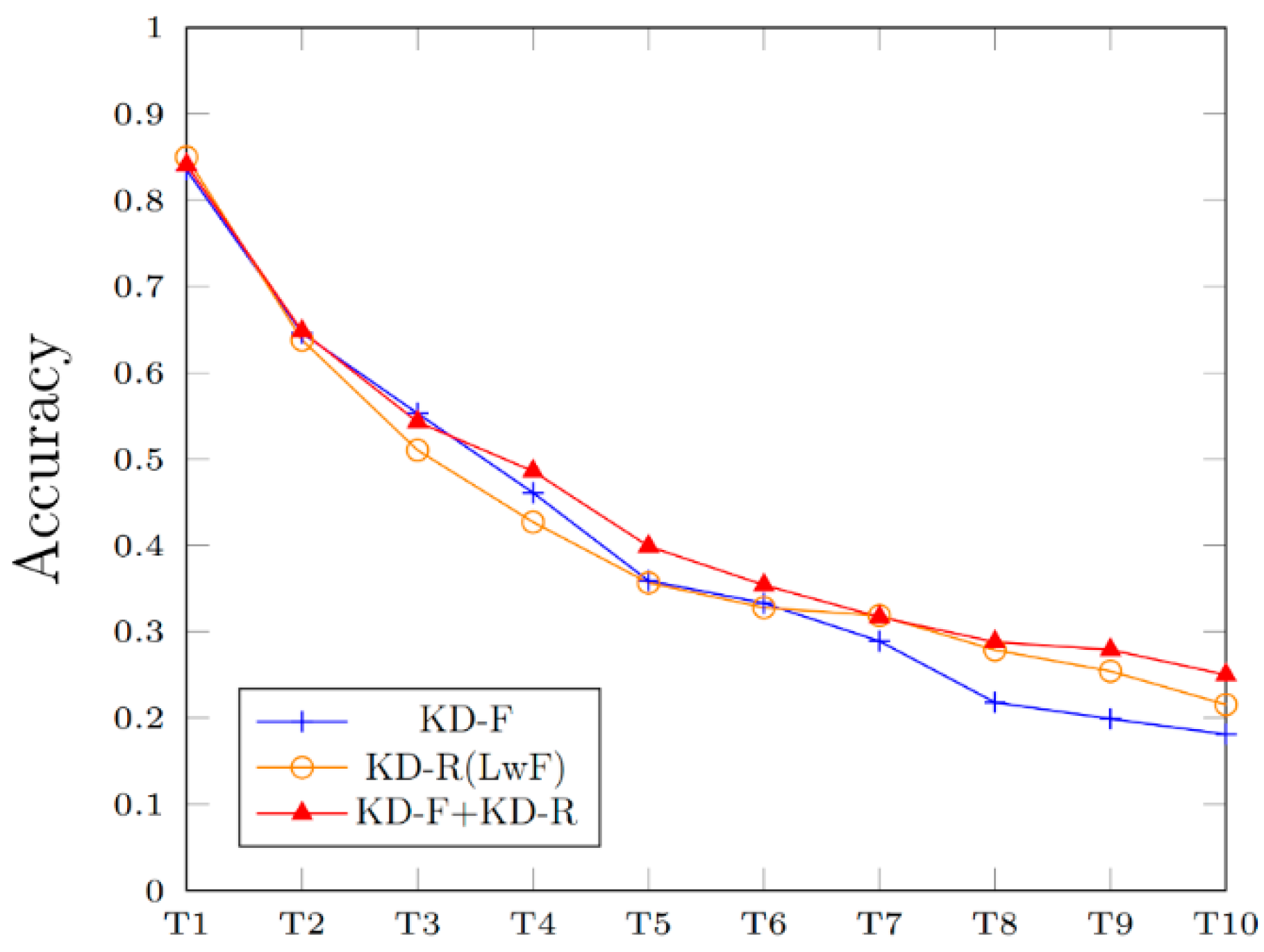
To address the issue of catastrophic forgetting, this study proposes employing dual knowledge distillation to preserve the model’s ability to retain knowledge of previous tasks. The CIFAR100 dataset was utilized in this experiment. Figure 4 presents a comparison of accuracy using different types of knowledge distillation during the first stage. Three approaches were considered: adopting only KD-F, adopting only KD-R, which corresponds to the baseline method LwF [18], and adopting both KD-F and KD-R. In this experiment, the weight α in all three methods was set to 2. The results in Figure 4 demonstrate that the accuracy is not as good as using dual distillation when only one distillation loss is considered. This is because calculating the knowledge distillation loss solely on the feature maps enables the new model to effectively capture the features of the old model, but the classifier cannot adapt to the changed feature space, resulting in forgetting old tasks. On the other hand, calculating the response-based loss solely on the logit output of the classifier may drastically change the feature space with the increasing number of tasks, leading the model to be unstable. When both distillation losses are considered, the feature space is retained, and the classifiers of new tasks are forced to learn from this feature space, while the classifiers for old tasks only make slight adjustments. This approach improves the overall accuracy. These findings suggest that the combination of KD-F with KD-R is the most effective approach in mitigating catastrophic forgetting. Thus, subsequent experiments were conducted using both KD-F and KD-R.

4.3. Confusions among Tasks

Due to the information imbalance between new and old tasks, the acquisition of new task knowledge relies on the strong supervisory signal provided by the cross-entropy loss, while knowledge distillation is employed for acquiring old task knowledge. It has been observed by Zhao et al. [49] that while knowledge distillation effectively retains knowledge of old tasks and reduces misclassification of old task categories as other old task categories, it also increases the likelihood of misclassifying old task categories as new task categories. This is attributed to the limited scope of distillation loss calculation within old task categories. Consequently, even if an old task sample is misclassified as a new task category, the distillation loss may remain low. Conversely, if an old task sample is misclassified as a different old task category, the distillation loss becomes significant. Despite the classifier providing sufficiently large logits for old task categories, the logits of old task samples are unable to surpass the logits of new categories due to the larger logits associated with the new task categories. This phenomenon is termed “old–new confusion” (ONC) [50], and it has been observed in this study as well.

To overcome the ONC problem, Ahn et al. [51] proposed the Separated Softmax (SS) method. The SS method segregates the model output of the new task and the old task. The final prediction given a test sample x is obtained using

$$\widehat{y}=\arg \underset{t=1:T}{\max }{z}_t\left(x,{\mathsf{\theta }}_t\right),$$

(10)

where $z_t$ is the output logits of the classifier ${\mathsf{\theta }}_t$. This technique serves to prevent the mixing of logits from the old task with the classes of the new task during the calculation of output probabilities. Another approach, called Weight Alignment (WA) [49], normalizes the weights of the last fully connected layers (i.e., classifiers) between the old tasks and new tasks (see Equations (11) and (12)). This ensures fairness in the output logits for both the new task and the old task.

$${\mathrm{W}}_{old}=\left({\mathrm{w}}_1,{\mathrm{w}}_2,\dots ,{\mathrm{w}}_{c_{old}}\right),{\mathrm{W}}_{new}=\left({\mathrm{w}}_{c_{old}+1},{\mathrm{w}}_{c_{old}+2},\dots ,{\mathrm{w}}_{c_{all}}\right)$$

(11)

and

$${\widehat{\mathrm{W}}}_{new}=\frac{mean\left(Norm\left({\mathrm{W}}_{old}\right)\right)}{mean\left(Norm({\mathrm{W}}_{new}\right))}·{\mathrm{W}}_{new}$$

(12)

where W_old is the classifier weights of old tasks, and W_new is the classifier weights of new tasks.

Considering the presence of the ONC phenomenon in this study, the experimental setup incorporates SS and WA techniques to explore the possibility of further improving performance. Results are shown in the next subsection.

4.4. Ablation Study

A comparative analysis was conducted to evaluate multiple methods, including the incorporation of WA and SS techniques, to address the ONC problem and assess their compatibility with the proposed method. When it comes to adopting WA and SS, we followed their original work without making any modifications. The detailed findings are presented in

Table 1. Comparisons of different combinations of methods on CIFAR100. The values in the table represent classification accuracies (%). S1 and S2 stand for the stages I and II proposed in this study. The letter “T” indicates the incremented task. The original two-stage design has better accuracy at tasks T1 and T2. However, the two-stage model with separated softmax achieves the highest accuracy after task T3. Numbers in bold indicate the highest accuracy among all methods in the corresponding tasks.

Method	T0	T1	T2	T3	T4	T5	T6	T7	T8	T9
LwF [18]	87.4	73.7	58.7	21.7	17.6	16.2	16.0	16.3	14.6	14.2
LwF + WA [49]	89.3	73.3	63.1	23.7	21.0	18.0	17.5	16.3	14.3	14.6
S1	88.6	73.5	61.3	49.1	27.7	23.3	21.7	20.6	19.7	18.6
S1 + WA	86.2	70.1	58.9	45.5	35.3	26.2	22.9	21.9	18.7	17.3
S1 + S2	87.7	75.6	64.8	49.6	36.2	27.7	23.1	21.3	19.8	19.9
S1 + S2 + WA	87.0	73.2	60.1	48.4	33.2	10.1	12.1	13.2	12.6	11.2
S1 + SS	88.6	72.2	59.2	47.9	28.2	24.6	23.3	20.9	20.2	20.3
S1 + WA + SS	86.2	70.6	59.0	46.3	36.3	26.1	23.9	22.3	18.8	17.5
S1 + S2 + SS	87.7	74.1	63.7	50.4	37.8	29.4	25.8	23.4	21.2	21.1
S1 + S2 + WA + SS	87.0	71.7	60.2	48.5	33.9	10.9	12.7	13.2	12.8	11.5

and

Table 2. Comparisons of different combinations of methods on RESISC45. The values in the table represent classification accuracies (%). Numbers in bold indicate the highest accuracy among all methods in the corresponding tasks.

Method	T0	T1	T2	T3	T4
LwF [18]	91.9	74.0	66.5	61.2	55.7
LwF + WA [49]	93.1	74.6	67.7	63.9	55.3
S1	92.4	74.8	66.9	63.2	55.8
S1 + WA	92.4	72.5	64.4	58.8	54.3
S1 + S2	92.1	74.8	67.7	64.6	57.3
S1 + S2 + WA	92.6	73.8	63.0	60.1	55.7
S1 + SS	92.4	74.7	66.2	61.2	57.6
S1 + WA + SS	92.4	73.1	65.0	59.1	54.5
S1 + S2 + SS	92.1	75.0	67.1	61.9	57.1
S1 + S2 + WA + SS	92.6	74.5	64.4	60.4	56.6

, where T0 represents the initial task, and T1 represents the first incremented task, and so on. The CIFAR100 dataset was partitioned into ten tasks due to its abundant sample size, while the RESISC45 dataset was divided into five tasks due to its comparatively smaller sample size. It should be noted that the proposed method comprises two stages, where the first stage (referred to as S1) can be independently trained, while the second stage (referred to as S2) needs to be conducted following S1. The experimental results in Table 1 indicate that either WA or SS, in conjunction with the proposed two-stage design, contributes to an overall improvement in top-1 accuracy. However, the simultaneous utilization of WA and SS does not yield a significant effect. In addition, the adoption of the two-stage approach proposed in this study demonstrates superior accuracy compared to solely employing the first stage in tasks T1 and T2. It is noteworthy that the incorporation of SS in conjunction with the two-stage approach achieves the highest accuracy after task T3, whereas the incorporation of WA lowers the overall accuracy significantly.

When experimenting with the RESISC45 dataset, it was observed that, due to its relatively small size, most combinations resulted in acceptable classification accuracy. As a result, the effectiveness of the proposed method was not significantly proven. However, the two-stage design with SS still yielded favorable results compared to adopting stage I solely. These results lead to the conclusion that for long-term incremental tasks, the implementation of the two-stage approach can effectively enhance the overall effectiveness of recognition, particularly through SS.

4.5. Forgetting Rate

To evaluate the severity of catastrophic forgetting in the model, we refer to the study conducted by Chaudhry et al. [52] to assess the level of forgetting of previous tasks by the model in the current task. The forgetting rate measures the difference between the highest accuracy achieved for a specific task among previous tasks and the accuracy of that task when the current incremented task is involved. Based on this definition, when the model undergoes incremental training on task t, the forgetting rate for the jth task, $f_j^t$, is calculated using the following equations:

$$f_j^t=\underset{i\in \{1,\dots ,t-1\}}{\mathit{max}}(a_{i,j}-a_{t,j}),\forall j<t$$

(13)

and

$${\mathcal{F}}^t=\frac{1}{t-1}{\sum }_{j=1}^{t-1}{f}_j^t,$$

(14)

where $a_{i,j}$ is the averaged classification accuracy of task j when there are I tasks in total. The overall forgetting rate ${\mathcal{F}}^t$ is the averaged value for all previous tasks. A lower ${\mathcal{F}}^t$ indicates a smaller level of forgetting. The forgetting rates of various combinations are calculated for the CIFAR100 and RESISC45 datasets and are presented in

Table 3. Comparisons of the forgetting rate (%) of different methods on CIFAR100. Smaller numbers indicate better performance. Numbers in bold indicate the highest accuracy among all methods in the corresponding tasks.

Method	T1	T2	T3	T4	T5	T6	T7	T8	T9
LwF [18]	23.7	37.8	64.5	60.4	56.9	54.1	52.1	51.9	51.8
LwF + WA [49]	8.2	36.1	44.7	41.5	41.2	42.2	40.0	39.9	41.2
S1	20.8	28.8	33.8	53.6	53.5	53.5	52.4	51.2	52.3
S1 + WA	5.3	13.1	23.3	30.7	37.5	39.8	39.3	42.9	45.3
S1 + S2	18.5	23.8	36.8	46.8	52.0	55.4	54.7	54.1	53.1
S1 + S2 + WA	8.2	15.3	21.8	36.7	54.1	49.4	46.8	45.5	46.5
S1 + SS	21.4	28.3	30.3	47.9	46.4	45.9	45.6	44.1	43.9
S1 + WA + SS	9.1	18.5	23.9	31.1	39.0	39.4	39.8	42.9	45.1
S1 + S2 + SS	17.7	21.8	28.9	39.3	44.5	46.3	46.2	47.0	46.7
S1 + S2 + WA + SS	10.1	17.6	22.2	35.75	54.5	49.7	47.0	46.1	46.5

and

Table 4. Comparisons of the forgetting rate (%) of different methods on RESISC45. Smaller numbers indicate better performance. Numbers in bold indicate the highest accuracy among all methods in the corresponding tasks.

Method	T1	T2	T3	T4
LwF [18]	8.7	16.5	26.0	29.8
LwF + WA [49]	19.1	18.4	21.9	32.2
S1	15.1	15.5	16.5	25.1
S1 + WA	2.9	5.8	7.6	12.6
S1 + S2	9.8	10.9	10.9	13.0
S1 + S2 + WA	3.7	7.7	8.1	13.1
S1 + SS	13.1	15.4	14.9	18.3
S1 + WA + SS	5.6	7.2	8.5	13.4
S1 + S2 + SS	11.1	12.1	13.3	18.0
S1 + S2 + WA + SS	6.3	10.9	10.5	13.8

. It is observed that the inclusion of WA leads to a low forgetting rate; however, it also restricts the model’s flexibility, limiting its ability to learn new tasks and subsequently lowering classification accuracy (as indicated in Table 1 and Table 2). Therefore, based on the consistent findings in Table 3 and Table 4, we believe that the proposed two-stage approach with SS achieves a sufficiently low forgetting rate. Specifically, it demonstrates a reduction in the forgetting rate of 5.1% and 11.8% when compared to the baseline method LwF after the completion of nine incremented tasks on CIFAR100 and RESISC45 datasets, respectively. Moreover, this approach maintains the highest classification accuracy, surpassing LwF by 6.9% and 1.4% on both datasets, respectively.

5. Conclusions and Future Work

This study presents a novel incremental learning method that combines knowledge distillation and multiple classifiers. The proposed method is applied to address natural image classification and remote sensing image classification problems through a two-stage training process. In the first stage, a feature map-based knowledge distillation method is introduced, which transfers knowledge through the feature representation of the model’s feature extraction layer. This allows the feature space of the new model to approach the feature space of the old model, reducing the risk of catastrophic forgetting. However, relying solely on feature-based knowledge distillation may hinder the adaptability of the old task classifiers to changes in the feature space, resulting in weakened knowledge retention for the old task after consecutive tasks. To address the limitations of feature map-based knowledge distillation, this study introduces response-based knowledge distillation as a second form of knowledge transfer to alleviate catastrophic forgetting of the old task. The experiments conducted demonstrate that the proposed method is more effective in mitigating catastrophic forgetting compared to using response-based knowledge distillation or feature-based knowledge distillation alone.

However, using multiple distillation methods poses a “stability–plasticity dilemma”, limiting the model’s ability to learn new tasks while retaining old knowledge. To overcome this, the second stage of training incorporates multiple classifiers into the model and maximizes the differences among them on the new task. This approach aims to enhance the classification capability and robustness for the new task by maximizing the distinct information captured by each classifier while minimizing the overall classification error, thereby achieving a balance between stability and plasticity. The experimental results demonstrate the efficacy of the proposed method in addressing the “stability–plasticity dilemma”, which is the primary challenge encountered in incremental learning.

While the proposed method effectively mitigates catastrophic forgetting, there remains an issue of asymmetry between the information of the new and old tasks. To overcome this, we additionally employ the Separated Softmax and Weight Alignment techniques, and our findings indicate that the proposed method exhibits capability with both approaches, with the incorporation of Separated Softmax yielding the best results. Future research can explore further experiments on various datasets to examine the capacity of tasks, including factors such as the number of tasks and the number of classes in each task. In the context of remote sensing image classification problems, training models in the remote sensing domain often prove challenging due to sample scarcity and imbalance. Therefore, future research can investigate the generalizability of this study by incorporating additional techniques, such as data augmentation. Furthermore, other influencing factors, such as the impact of different OOD datasets on model learning and the relationship between the similarity of the new task and the OOD datasets, can also be explored.

References

- Li, J.; Wu, Y.; Zhang, H.; Wang, H. A Novel Unsupervised Segmentation Method of Canopy Images from UAV Based on Hybrid Attention Mechanism. Electronics 2023, 12, 4682. [Google Scholar] [CrossRef]
- McCloskey, M.; Cohen, N.J. Catastrophic interference in connectionist networks: The sequential learning problem. In Psychology of Learning and Motivation; Elsevier: Amsterdam, The Netherlands, 1989; pp. 109–165. [Google Scholar]
- Devkota, N.; Kim, B.W. Deep Learning-Based Small Target Detection for Satellite–Ground Free Space Optical Communications. Electronics 2023, 12, 4701. [Google Scholar] [CrossRef]
- Ma, S.; Chen, J.; Wu, S.; Li, Y. Landslide Susceptibility Prediction Using Machine Learning Methods: A Case Study of Landslides in the Yinghu Lake Basin in Shaanxi. Sustainability 2023, 15, 15836. [Google Scholar] [CrossRef]
- van de Ven, G.M.; Tuytelaars, T.; Tolias, A.S. Three types of incremental learning. Nat. Mach. Intell. 2022, 4, 1185–1197. [Google Scholar] [CrossRef]
- Mirza, M.J.; Masana, M.; Possegger, H.; Bischof, H. An efficient domain-incremental learning approach to drive in all weather conditions. In Proceedings of the IEEE/CVF Conference on Computer Vision and Pattern Recognition (CVPR) Workshops, New Orleans, LA, USA, 19–20 June 2022. [Google Scholar] [CrossRef]
- von Oswald, J.; Henning, C.; Sacramento, J.; Grewe, B.F. Continual learning with hypernetworks. In Proceedings of the International Conference on Learning Representations, Virtual Conference, 26–30 April 2020. [Google Scholar] [CrossRef]
- Van de Ven, G.M.; Siegelmann, H.T.; Tolias, A.S. Brain-inspired replay for continual learning with artificial neural networks. Nat. Commun. 2020, 11, 4069. [Google Scholar] [CrossRef]
- De Lange, M.; Aljundi, R.; Masana, M.; Parisot, S.; Jia, X.; Leonardis, A.; Slabaugh, G.; Tuytelaars, T. A continual learning survey: Defying forgetting in classification tasks. IEEE Trans. Pattern Anal. Mach. Intell. 2021, 44, 3366–3385. [Google Scholar] [CrossRef]
- Rebuffi, S.-A.; Kolesnikov, A.; Sperl, G.; Lampert, C.H. iCaRL: Incremental Classifier and Representation Learning. In Proceedings of the Conference on Computer Vision and Pattern Recognition, Honolulu, HI, USA, 21–26 July 2017. [Google Scholar] [CrossRef]
- Shin, H.; Lee, J.K.; Kim, J.; Kim, J. Continual learning with deep generative replay. In Proceedings of the Neural Information Processing Systems, Long Beach, CA, USA, 4–9 December 2017. [Google Scholar] [CrossRef]
- Lopez-Paz, D.; Ranzato, M. Gradient episodic memory for continual learning. In Proceedings of the Neural Information Processing Systems, Long Beach, CA, USA, 4–9 December 2017. [Google Scholar] [CrossRef]
- Rusu, A.A.; Rabinowitz, N.C.; Desjardins, G.; Soyer, H.; Kirkpatrick, J.; Kavukcuoglu, K.; Pascanu, R.; Hadsell, R. Progressive neural networks. arXiv 2016, arXiv:1606.04671. [Google Scholar] [CrossRef]
- Xu, J.; Zhu, Z. Reinforced continual learning. In Proceedings of the Neural Information Processing Systems, Montréal, QC, Canada, 3–8 December 2018. [Google Scholar]
- Fernando, C.; Banarse, D.S.; Blundell, C.; Zwols, Y.; Ha, D.R.; Rusu, A.A.; Pritzel, A.; Wierstra, D. PathNet: Evolution Channels Gradient Descent in Super Neural Networks. arXiv 2017, arXiv:1701.08734. [Google Scholar] [CrossRef]
- Mallya, A.; Lazebnik, S. PackNet: Adding multiple tasks to a single network by iterative pruning. In Proceedings of the Conference on Computer Vision and Pattern Recognition, Salt Lake City, UT, USA, 18–22 June 2018. [Google Scholar] [CrossRef]
- Serra, J.; Suris, D.; Miron, M.; Karatzoglou, A. Overcoming catastrophic forgetting with hard attention to the task. In Proceedings of the International Conference on Machine Learning, Vancouver, BC, Canada, 30 April–3 May 2018. [Google Scholar] [CrossRef]
- Li, Z.; Hoiem, D. Learning without forgetting. IEEE Trans. Pattern Anal. Mach. Intell. 2018, 40, 2935–2947. [Google Scholar] [CrossRef] [PubMed]
- Kirkpatrick, J.; Pascanu, R.; Rabinowitz, N.; Veness, J.; Desjardins, G.; Rusu, A.A.; Milan, K.; Quan, J.; Ramalho, T.; GrabskaBarwinska, A.; et al. Overcoming catastrophic forgetting in neural networks. Proc. Natl. Acad. Sci. USA 2017, 144, 3521–3526. [Google Scholar] [CrossRef] [PubMed]
- Bucilua, C.; Caruana, R.; Niculescu-Mizil, A. Model compression. In Proceedings of the 12th ACM SIGKDD International Conference on Knowledge Discovery and Data Mining, Philadelphia, PA, USA, 20–23 August 2006. [Google Scholar]
- Hinton, G.; Vinyals, O.; Deans, J. Distilling the knowledge in a neural network. In Proceedings of the NIPS Deep Learning and Representation Learning Workshop, Montréal, QC, Canada, 7–12 December 2015. [Google Scholar] [CrossRef]
- Kim, J.; Park, S.; Kwak, N. Paraphrasing complex network: Network compression via factor transfer. In Proceedings of the Neural Information Processing Systems, Montréal, QC, Canada, 3–8 December 2018. [Google Scholar] [CrossRef]
- Ba, L.J.; Caruana, R. Do Deep nets really need to be deep? In Proceedings of the Neural Information Processing Systems, Montréal, QC, Canada, 8–13 December 2014. [Google Scholar] [CrossRef]
- Mirzadeh, S.I.; Farajtabar, M.; Li, A.; Ghasemzadeh, H. Improved knowledge distillation via teacher assistant. In Proceedings of the AAAI Conference on Artificial Intelligence, New York, NY, USA, 7–12 February 2020. [Google Scholar] [CrossRef]
- Huang, Z.; Wang, N. Like What You Like: Knowledge Distill via Neuron Selectivity Transfer. arXiv 2017, arXiv:1707.01219. [Google Scholar] [CrossRef]
- Ahn, S.; Hu, S.; Damianou, A.; Lawrence, N.D.; Dai, Z. Variational information distillation for knowledge transfer. In Proceedings of the IEEE/CVF Conference on Computer Vision and Pattern Recognition, Long Beach, CA, USA, 16–20 June 2019. [Google Scholar] [CrossRef]
- Heo, B.; Lee, M.; Yun, S.; Choi, J.Y. Knowledge transfer via distillation of activation boundaries formed by hidden neurons. In Proceedings of the the AAAI Conference on Artificial Intelligence, Honolulu, HI, USA, 27 January–1 February 2019. [Google Scholar] [CrossRef]
- Zagoruyko, S.; Komodakis, N. Paying more attention to attention: Improving the performance of convolutional neural networks via attention transfer. In Proceedings of the International Conference on Learning Representations, Toulon, France, 24–26 April 2017. [Google Scholar] [CrossRef]
- Gou, J.; Yu, B.; Maybank, S.J.; Tao, D. Knowledge Distillation: A Survey. Int. J. Comput. Vis. 2021, 129, 1789–1819. [Google Scholar] [CrossRef]
- Chen, G.; Choi, W.; Yu, X.; Han, T.; Chandraker, M. Learning efficient object detection models with knowledge distillation. In Proceedings of the Neural Information Processing Systems, Long Beach, CA, USA, 4–9 December 2017. [Google Scholar] [CrossRef]
- Romero, A.; Ballas, N.; Kahou, S.E.; Chassang, A.; Gatta, C.; Bengio, Y. FitNets: Hints for thin deep nets. In Proceedings of the International Conference on Learning Representations, San Diego, CA, USA, 7–9 May 2015. [Google Scholar] [CrossRef]
- Passban, P.; Wu, Y.; Rezagholizadeh, M.; Liu, Q. ALP-KD: Attention-based layer projection for knowledge distillation. In Proceedings of the AAAI Conference on Artificial Intelligence, Vancouver, BC, Canada, 2–9 February 2021. [Google Scholar] [CrossRef]
- Chen, D.; Mei, J.P.; Zhang, Y.; Wang, C.; Wang, Z.; Feng, Y.; Chen, C. Cross-layer distillation with semantic calibration. In Proceedings of the AAAI Conference on Artificial Intelligence, Vancouver, BC, Canada, 2–9 February 2021. [Google Scholar] [CrossRef]
- Wang, X.; Fu, T.; Liao, S.; Wang, S.; Lei, Z.; Mei, T. Exclusivity-consistency regularized knowledge distillation for face recognition. In Proceedings of the european conference on computer vision, Glasgow, UK, 23–28 August 2020. [Google Scholar] [CrossRef]
- Liu, Y.; Cao, J.; Li, B.; Yuan, C.; Hu, W.; Li, Y.; Duan, Y. Knowledge distillation via instance relationship graph. In Proceedings of the IEEE/CVF Conference on Computer Vision and Pattern Recognition, Long Beach, CA, USA, 16–20 June 2019. [Google Scholar] [CrossRef]
- Csurka, G. A comprehensive survey on domain adaptation for visual applications. In Domain Adaptation in Computer Vision Applications; Springer: New York, NY, USA, 2017; pp. 1–35. [Google Scholar] [CrossRef]
- Zhang, J.; Liang, C.; Kuo, C.C.J. A fully convolutional tri-branch network (FCTN) for domain adaptation. In Proceedings of the IEEE International Conference on Acoustics, Speech and Signal Processing (ICASSP), Calgary, AB, Canada, 15–20 April 2018. [Google Scholar] [CrossRef]
- Chapelle, O.; Scholkopf, B.; Zien, A. Semi-supervised learning. IEEE Trans. Neural Netw. 2009, 20, 542. [Google Scholar] [CrossRef]
- Zhu, X. Semi-supervised learning literature survey. In Computer Science; University of Wisconsin-Madison: Madison, WI, USA, 2006; Volume 2, p. 4. [Google Scholar]
- Raina, R.; Battle, A.; Lee, H.; Packer, B.; Ng, A.Y. Self-taught learning: Transfer learning from unlabeled data. In Proceedings of the 24th International Conference on Machine Learning, Corvallis, OR, USA, 20–24 June 2007. [Google Scholar]
- Yu, Q.; Aizawa, K. Unsupervised out-of-distribution detection by maximum classifier discrepancy. In Proceedings of the IEEE/CVF International Conference on Computer Vision, Seoul, Republic of Korea, 27 October–2 November 2019. [Google Scholar] [CrossRef]
- Saito, K.; Watanabe, K.; Ushiku, Y.; Harada, T. Maximum classifier discrepancy for unsupervised domain adaptation. In Proceedings of the IEEE conference on Computer Vision and Pattern Recognition, Salt Lake City, UT, USA, 18–22 June 2018. [Google Scholar] [CrossRef]
- Krizhevsky, A. Learning Multiple Layers of Features from Tiny Images; Technical report; University of Toronto: Toronto, ON, Canada, 2009. [Google Scholar]
- Le, Y.; Yang, X. Tiny Imagenet Visual Recognition Challenge; Stanford University: Stanford, CA, USA, 2015. [Google Scholar]
- Cheng, G.; Han, J.; Lu, X. Remote Sensing Image Scene Classification: Benchmark and State of the Art. Proc. IEEE 2017, 105, 1865–1883. [Google Scholar] [CrossRef]
- Yang, Y.; Shawn, N. Bag-of-visual-words and spatial extensions for land-use classification. In Proceedings of the 18th SIGSPATIAL International Conference on Advances in Geographic Information Systems (GIS ’10), San Jose, CA, USA, 2–5 November 2010. [Google Scholar]
- Xia, G.S.; Hu, J.; Hu, F.; Shi, B.; Bai, X.; Zhong, Y.; Lu, X.Q. AID: A Benchmark Data Set for Performance Evaluation of Aerial Scene Classification. IEEE Trans. Geosci. Remote Sens. 2017, 55, 3965–3981. [Google Scholar] [CrossRef]
- He, K.; Zhang, X.; Ren, S.; Sun, J. Deep residual learning for image recognition. In Proceedings of the IEEE Conference on Computer Vision and Pattern Recognition (CVPR), Las Vegas, NV, USA, 26 June–1 July 2016. [Google Scholar] [CrossRef]
- Zhao, B.; Xiao, X.; Gan, G.; Zhang, B.; Xia, S.-T. Maintaining Discrimination and fairness in class incremental learning. In Proceedings of the IEEE/CVF Conference on Computer Vision and Pattern Recognition (CVPR), Seattle, WA, USA, 13–19 June 2020. [Google Scholar] [CrossRef]
- Huang, B.; Chen, Z.; Zhou, P.; Chen, J.; Wu, Z. Resolving task confusion in dynamic expansion architectures for class incremental learning. In Proceedings of the AAAI Conference on Artificial Intelligence, Washington, DC, USA, 7–14 February 2023. [Google Scholar] [CrossRef]
- Ahn, H.; Kwak, J.; Lim, S.; Bang, H.; Kim, H.; Moon, T. SS-IL: Separated softmax for incremental learning. In Proceedings of the International Conference on Computer Vision (ICCV), Montreal, QC, Canada, 10–17 October 2021. [Google Scholar] [CrossRef]
- Chaudhry, A.; Dokania, P.K.; Ajanthan, T.; Torr, P.H. Riemannian walk for incremental learning: Understanding forgetting and intransigence. In Proceedings of the European Conference on Computer Vision (ECCV), Munich, Germany, 8–14 September 2018. [Google Scholar] [CrossRef]