Explaining the Behaviour of Reinforcement Learning Agents in a Multi-Agent Cooperative Environment Using Policy Graphs ^†

Abstract

The adoption of algorithms based on Artificial Intelligence (AI) has been rapidly increasing during the last few years. However, some aspects of AI techniques are under heavy scrutiny. For instance, in many use cases, it is not clear whether the decisions of an algorithm are well informed and conforming to human understanding. Having ways to address these concerns is crucial in many domains, especially whenever humans and intelligent (physical or virtual) agents must cooperate in a shared environment. In this paper, we apply an explainability method based on the creation of a Policy Graph (PG) based on discrete predicates that represent and explain a trained agent’s behaviour in a multi-agent cooperative environment. We show that from these policy graphs, policies for surrogate interpretable agents can be automatically generated. These policies can be used to measure the reliability of the explanations enabled by the PGs through a fair behavioural comparison between the original opaque agent and the surrogate one. The contributions of this paper represent the first use case of policy graphs in the context of explaining agent behaviour in cooperative multi-agent scenarios and present experimental results that sets this kind of scenario apart from previous implementations in single-agent scenarios: when requiring cooperative behaviour, predicates that allow representing observations about the other agents are crucial to replicate the opaque agent’s behaviour and increase the reliability of explanations.

1. Introduction and Motivation

Over the last decade, methods based on machine learning have achieved remarkable performance in many seemingly complex tasks such as image processing and generation, speech recognition or natural language processing. It is reasonable to assume that the range of potential applications will keep growing in the forthcoming years. However, there are still many concerns about the transparency, understandability and trustworthiness of systems built using these methods, especially when they are based on so-called opaque models [1]. For example, there is still a need for proper explanations of the behaviour of agents where their behaviour could be a risk for their real-world applicability and regulation in domains such as autonomous driving, robots, chatbots, personal assistants, or recommendation, planning or tutoring systems [2,3].

Since AI has an increasing impact on people’s everyday lives, it becomes urgent to keep progressing in the field of Explainable Artificial Intelligence (XAI) [4]. In fact, there are already regulations in place that require AI model creators to enable mechanisms that can produce explanations for them, such as the European Union’s General Data Protection Regulation (GDPR) that went into effect on 25 May 2018 [5]. This law creates a “Right to Explanation” whereby a user can ask for the explanation of an algorithmic decision that was made about them. Therefore, explainability is not only desirable but is also a frequent requirement and, in cases where personal data are involved, it is mandatory. Furthermore, the European AI Act [6] prescribes that AI systems presenting risks, such as those that interact with humans and therefore may impact safety, must be transparent. Cooperation between humans and AIs will gradually become more common [7], and thus it is crucial to be able to explain the behaviour of cooperative agents so that their actions are understandable and can be trusted by humans. However, in many cases, agents trained to operate and cooperate in physical or virtual environments use Reinforcement Learning (RL) complex models such as deep neural networks that are opaque by nature. Due to this need for being able to make such systems more transparent, explainability in RL (XRL) is starting to gain momentum as a distinct field of explainability.

This paper aims to contribute to XRL by building upon the line of research opened in [8,9], which has consisted of producing explanations from predicate-based Policy Graphs (PGs) generated from the observation of RL-trained agents in single-agent environments. This paper is an extension of the conference paper [10] (Vila et al., ”Testing Reinforcement Learning Explainability Methods in a Multi-agent Cooperative Environment.” Published in: Artificial Intelligence Research and Development 355 A. Cortés et al. (Eds.) © 2022 The authors and IOS Press. This article is published online with Open Access by IOS Press and distributed under the terms of the Creative Commons Attribution Non-Commercial License 4.0 (CC BY-NC 4.0). doi:10.3233/ FAIA220358), in which we present the first use case of the same methodology to generate explanations for agents trained with Multi-Agent Reinforcement Learning (MARL) methods in a cooperative environment. The contributions of this paper are focused on analysing what kind of explanations can be produced and whether there can be explanations about the relationship between the agents, i.e., about cooperation.

Currently, there are several approaches to explain agents trained with reinforcement learning, which are mainly from a single-agent perspective. In this work, we briefly overview some of them in Section 2 and we introduce the approach followed in our use case, which is based on the creation of policy graphs. We briefly summarise our initial results of applying such an approach to a single-agent environment in Section 2.1. In Section 3, we introduce a multi-agent cooperative environment, which we use in Section 4 to apply our explainability method, giving some insights about the required methodology to generate explanations in a new domain. In Section 5, we introduce three algorithms that query policy graphs. In Section 6, we build new agents using the graph as a policy to compare them with the originals in order to have a measure of reliability for the explanations. Finally, we end with a summary of the main conclusions and contributions from the work in Section 7.

2. Background

The area of explainability in reinforcement learning is still relatively new, especially when dealing with policies as opaque models. In this section, we will provide a brief overview of some state-of-the-art XRL methods and discuss, in more depth, the method chosen for our work. A more detailed study of the explainability methods in RL can be found in [11]: XRL methods can be classified by their time horizon of explanation (reactive/proactive), scope of explanation (global/local), timing of explanation (post hoc /intrinsic), type of the environment (deterministic/stochastic), type of policy (deterministic/stochastic) and their agent cardinality (single-agent/multi-agent system).

Reactive explanations are those that are focused on the immediate moment. A family of reactive methods is policy simplification, which finds solutions based on tree structures. In these, the agent answers the questions from the root to the bottom of the tree in order to decide which action to execute. For instance, Coppens et al. [12] use Soft Decision Trees (SFTs), which are structures that work similarly to binary trees but where each decision node works as a single perceptron that returns, for a given input x, the probability of going right or left. This allows the model to learn a hierarchy of filters in its decision nodes. Another family is reward decomposition, which tries to decompose the reward into meaningful components. In [13], Juozapaitis et al. decompose the Q-function into reward types to try to explain why an action is preferred over another. With this, they can know whether the agent is choosing an action to be closer to the objective or to avoid penalties. Another approach is feature contribution and visual methods, like LIME [14] or SHAP [15], which try to find which of the model features are the most relevant in order to make decisions. On the other hand, Greydanus et al. [16] differentiate between gradient-based and perturbation-based saliency methods. The former try to answer the question “Which features are the most relevant to decide the output?” while the latter are based on the idea of perturbing the input of the model in order to analyse how its predictions changes.

Proactive models are those that focus on longer-term consequences. One possible approach is to analyse the relationships between variables. This family of techniques give explanations that are very close to humans because we see the world through a causal lens [17]. According to [18], the causal model tries to describe the world using random variables. Each of these variables has a causal influence on the others. This influence is modelled through a set of structural equations. Madumal et al. [19] generate explanations of behaviour based on a counterfactual analysis of the structural causal model that is learned during RL. Another approach tries to break down one task into multiple subtasks in order to represent different abstraction levels [20]. Therefore, each task can only be carried out if its predecessor tasks have been finished.

According to [21], in order to achieve interoperability, it is important that the tasks are described by humans beforehand. For instance, Kulkarni et al. [20] define two different policies in hierarchical RL, local and global policies. The first one uses atomic actions in order to achieve the subobjectives, while the second one uses the local policies in order to achieve the final goal.

In addition, there is another approach that combines relational learning or inductive logic programming with RL. The idea behind these methods [22] is to represent states, actions and policies using first-order (or relational) language. Thanks to this, it is easier to generalise over goals, states and actions, exploiting knowledge learnt during an earlier learning phase.

Finally, another approach consists of building a Markov Decision Process and following the graph from the input state to the main reward state [19]. This allows asking simple questions about the chosen actions. As an optional step, we can simplify the state representation (discretising it if needed). This step becomes crucial when we are talking about more complex environments [8]. In this work, we will use this last approach: we will use a method that consists of building a policy graph by mapping the original state to a set of predicates (discretisation step) and then repeatedly running the agent policy, recording its interactions with the environment. This graph of states and actions can then be used for answering simple questions about the agent’s execution, which is shown at the end of Section 4. This is a post hoc and proactive method, with a global scope of explanation, which works with both stochastic environments and policies and has, until the use case presented in this paper, only been tested in single-agent environments (

Table 1. Summarised comparison of XRL methods with policy graphs according to the taxonomy presented in Krajna et al. [11] (i.e., respectively, time horizon, scope, timing, types of environment and policy and agent cardinality). A more complete description of each method can be found in the cited paper. Env. stands for type of environment (stochastic/deterministic), while P-H stands for post hoc and Intr. stands for intrinsic.

Method	Horiz.	Scope	Timing	Env.	Policy	Agents	Description
Coppens et al. [12]	Reac.	Global	P-H	Stoch.	Stoch.	Single	Binary decision trees, value heatmap images
Juozapaitis et al. [13]	Reac.	Local	P-H	Stoch.	Deter.	Single	Decomposed reward diagrams and images
Greydanus et al. [16]	Reac.	Global	P-H	Deter.	Deter.	Multi-	Attention saliency maps
Madumal et al. [19]	Proac.	Local	P-H	Stoch.	Stoch.	Multi-	Counterfactual text explanations
Kulkarni et al. [20]	Proac.	Local	Intr.	Stoch.	Stoch.	Multi-	Attention saliency maps
Zambaldi et al. [22]	Proac.	Local	Intr.	Stoch.	Stoch.	Multi-	Counterfactual text explanations
Policy graphs	Proac.	Global	P-H	Stoch.	Stoch.	Sing./Mult.	Behaviour graphs, text explanations, transparent agent version

).

Thus, a policy graph is built by sampling the behaviour of a trained agent in the environment in the form of a labelled directed graph $PG=\langle V,E,A\rangle$ where each node $v_i\in V$ represents a discretised state $s_i$, and each edge $e=(v_i,a,v_j)\in E$ represents the transition $(s_i,a,s_j)$, where $a\in A$ is an action from the available actions of the environment.

Note that for the sake of brevity, hereinafter, we equate discretised states and their node counterparts in a policy graph: $s_i=v_i\wedge V\subseteq S$, where S is the set of all discretised states.

There may exist more than one transition between the same pairs of nodes as long as the labels are different, as performing different actions in a certain state may still lead to the same resulting state. Conversely, there may exist more than one transition between a particular state and many different states labelled with the same action, since applying an action on the environment may have a stochastic effect (e.g., the action could occasionally fail).

Each node $v\in V$ stores the well-formed formula in propositional logic that represents its state and its probability $P\left(v\right)$. Each edge $e=(v_i,a,v_j)$ stores the action a that causes the transition it represents, and its probability $P(v_j,a|v_i)$, such that:

$$\forall v\in V,\exists e=(v,a,v^{\prime })\in E\Rightarrow \sum _{(v,a_i,v_j)\in E}P(v_j,a_i|v)=1$$

(1)

Essentially, for every node in the policy graph, either the sum of probabilities for every edge originating from the node is exactly 1, or the node has no such edges.

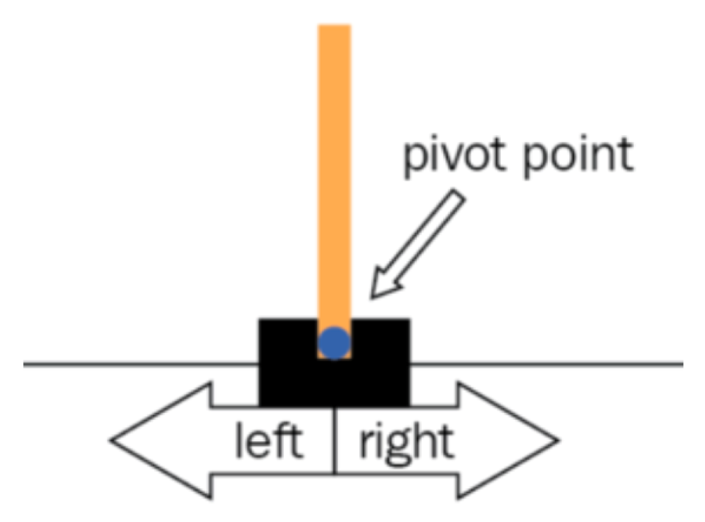
2.1. Explaining the Cartpole Scenario

Before detailing the use of policy graphs for explaining agents’ behaviour in a multi-agent cooperative setting, it may be worth describing first how this methodology can be applied to a single-agent setting.

In [9], we use Cartpole as the scenario for this work. Cartpole is an environment for reinforcement learning provided by the OpenAI Gym library (https://gym.openai.com, accessed on 4 December 2023), in which a pole is attached to a cart through an unactuated joint, and both move along a friction-less track, as depicted in Figure 1. The agent controls the cart by moving it left or right, and the challenge is to prevent the pole from falling over due to gravity. To represent the state of the system, the agent has access to observations containing four variables: cart position, cart velocity, pole angle, and pole angular velocity. A fall is determined when the pole angle exceeds 12 degrees from the vertical or when the cart moves out of bounds.

It was possible to generate valid and accurate explanations for this environment by using the following set of predicates as the discretiser for the policy graphs:

• $pole\_falling\left(X\right)$, where $X\in \{left,right\}$.
• $pole\_stabilising\left(X\right)$, where $X\in \{left,right\}$.
• $pole\_standing\_up\left(\right)$.
• $cart\_moving\left(X\right)$, where $X\in \{left,right\}$.
• $cart\_pos\left(X\right)$, where $X\in \{far\_left,far\_right,left,right\}$.
• $cart\_near\_middle\left(\right)$.
• $stuck\left(X\right)$, where $X\in \{left,right\}$.

This set of predicates, combined with the algorithms introduced in [8], allow for generating explanations for the behaviour of any agent operating in the Cartpole environment. This explanations can be validated via qualitative methods, e.g., by human expert validation. In order to validate these explanations from a quantitative perspective, our previous work [9] presented a novel technique based on the creation of a new agent policy inferred from the structure of the policy graph, trying to imitate the behaviour developed by the original trained agent’s policy.

One concern related to this proposal is that the policy graph is based on a simplification of the states and the actions (using predicates), and therefore such a policy could also be an oversimplification of a policy that is backed by a complex, opaque model. For this reason, our aim was to confirm whether the behaviour of the two policies shows a similar performance and, therefore, that the critical decisions that influence performance are comparable. If that is the case, the explanations generated would be able to reflect the trained agent in terms of human interpretation.

Figure 2 provides a histogram illustrating the final steps achieved by various policies. These final steps could be a consequence of either reaching success (200 steps) or encountering failure. Among these policies, the ones involving random agents (HRD 5.54% success rate and RND 0%) are severely outmatched by those considering either the original agent (DQN 78.65%), the policy graph (PGR 78.16%), or their hybrid (HEX 72.95%), the three of them having comparable success rates. Interestingly, the success rate of the PGR agent displays significant deviations in the initial steps, particularly around steps 25 to 50, as evidenced by non-marginal frequencies in the histogram. These deviations can be attributed to the previously mentioned state simplification and discretisation, affecting the agent’s ability to stabilise in challenging scenarios, such as when the pole is far from the center. In contrast, DQN and HEX, the latter being 50% based on PGR, showcase remarkably similar histograms, indicating that the PGR policy has a stable behaviour after 50 steps, aligning well with the original behaviour.

Additionally, we conducted a correlation analysis (Spearman) involving three domain-specific metrics: average cart movement, average pole velocity, and average pole rotation (as shown in Figure 3). The most significant correlations regarding cart movement are observed between DQN and HEX (0.60, p < 0.001) and between PGR and HEX (0.53, p < 0.001), which is logical since HEX is a combination of both policies. The correlation between DQN and PGR (0.26, p < 0.001) is statistically significant but relatively low. However, when examining the impact of actions on the pole, including velocity and rotation, higher correlations are identified: DQN and PGR (0.55, p < 0.001), DQN and HEX (0.72, p < 0.001), and PGR and HEX (0.67, p < 0.001).

Our analysis suggested that the behaviours of the two agents yield similar outcomes, both in terms of performance and their influence on the pole’s behaviour, in an environment where there is only one agent and therefore there are no actions from other agents to take into account. For further details on the methodology and the results of the quantitative analysis for the Cartpole environment, please refer to [9]. From now on, in this paper, we focus on the application of policy graphs to a multi-agent scenario, in which we analyse the feasibility of using policy graphs to explain the behaviour of agents in environments where the actions of other agents are relevant for the performance.

3. Overcooked-AI: A Multi-Agent Cooperative Environment

In this paper, we have used the PantheonRL [23] package for training and testing an agent in Overcooked-AI [24]. Overcooked-AI is a benchmark environment for fully cooperative human–AI task performance, which is based on the popular video game Overcooked (http://www.ghosttowngames.com/overcooked, accessed on 15 November 2023). The goal of the game is to deliver soups as fast as possible. Each soup requires placing up to three ingredients in a pot, waiting for the soup to cook, and then having an agent pick up the soup and deliver it. The agents should split up tasks on the fly and coordinate effectively in order to achieve high rewards.

The environment has a sparse reward function. In the steps where certain tasks of interest are performed, the following rewards are given: 3 points if an agent places an onion in a pot or if it takes a dish, 5 points if it takes a soup and 20 points if the soup is placed in a delivery area. The same reward is delivered to both agents without regard to which agent performed the task itself.

Here, in this work, we have worked with five different layouts: simple, unident_s, random0, random1 and random3 (Figure 4).

At each timestep, the environment returns a list with the objects not owned by the agent present in the layout and, for each player, the position, orientation, and object that it is holding and its information. We can also obtain the location of the basic objects (dispensers, etc.) at the start of the game.

For example, the agent would receive the following data from the situation depicted in Figure 5:

• Player 1: Position (5, 1)—Facing (1, 0)—Holding Soup;
• Player 2: Position (1, 3)—Facing (−1, 0)—Holding Onion;
• Not owned objects: Soup at (4, 0)—with 1 onion and 0 cooking time.

The environment layout can have a strong influence on the degree of cooperation and the strategy agents must follow in order to win the game or to have an optimal behaviour. For instance, unident_s has enough elements at each side of the kitchen for each agent to serve soups by themselves without the need of the other, so cooperation is not mandatory for winning, but it is desirable for optimality. On the other hand, random0 has different elements at each side of the layout division, so cooperation is mandatory for winning. random1 and random3 require that agents are capable of not blocking each other.

The aim of our work is not to solve the Overcooked game but rather to analyse the potential of explainability in this cooperative setting. Therefore, we do not really care about what method is used to train our agent. However, it is important that the agent performs reasonably well in order to verify that we are explaining an agent with a reasonable policy. Thus, we train our agents using Proximal Policy Optimisation (PPO) [25] because it has achieved great results in Overcooked previously [24]. We use the Stable Baselines 3 [26] Python package to train all agents. Indeed, if we obtain good results with PPO, we should also obtain good results with other methods since our explainability method is independent from the training algorithms used. In our case, we have trained five different agents (one for each layout) for 1M total timesteps and with an episode length of 400 steps. Training results can be found in

Table 2. Performance metrics of the trained agent pairs.

Layout	Mean Reward	Std.
simple	387.87	25.33
unident_s	757.71	53.03
random0	395.01	54.43
random1	266.01	48.11
random3	62.5	5.00

.

4. Building a Policy Graph for the Trained Agent

We have created a total of 10 predicates to represent each state. The first two predicates are held and held_partner, which have five possible values depending on which object the agent and its partner, respectively, are holding: O(nion), T(omato), D(ish), S(ervice) or * for nothing.

The third predicate is pot_state, which has four possible values depending on the state of each pot:

-

$"Of"$ (Off), when $[\mathrm{pot}.\mathrm{onions}=0]$.

-

$"Fi"$ (Finished), when $[\mathrm{pot}.\mathrm{onions}=3\wedge \mathrm{pot}.\mathrm{timer}\ge 20]$.

-

$"Co"$ (Cooking), when $[\mathrm{pot}.\mathrm{onions}=3\wedge \mathrm{pot}.\mathrm{timer}<20]$.

-

$"Wa"$ (Waiting), when $[\mathrm{pot}.\mathrm{onions}<3]$.

To relate the actions of the agent with the relative position of the objects in the environment, we introduce six more predicates: onion_pos(X), tomato_pos(X), dish_pos(X), pot_pos(X), service_pos(X) and soup_pos(X). All of them can have the same six possible values depending on the next action to perform to reach the corresponding object as quickly as possible: S(tay), R(ight), L(eft), T(op), B(ottom) or I(nteract). The last predicate is partner_zone, which is intended to represent agents’ cooperation along with held_partner. It has eight possible values depending on which cardinal point the partner is located at (e.g., “NE” for “northeast”).

As mentioned in Section 2, the aim of the policy graph algorithm is to apply the following method: to record all the interactions of the original trained agent by executing it in a large set of random environments and to build a graph relating predicate-based states seen in the environment with the actions executed by the agents after each of those states.

An example can be found in Figure 6. In this graph, the state on the left side represents the state {held(Dish), held_partner(Onion), pot_state(Finished), onion_pos(Interact), toma-to_pos(Stay), dish_pos(Stay), pot_pos(Top), service_pos(Right), soup_pos(Right), partner-_zone(South)}. The state on the right side represents the state {held(Dish), held_partner(Onion), pot_state(Finished), onion_pos(Left), tomato_pos(Stay), dish_pos(Stay), pot_pos(Left), service-_pos(Right), soup_pos(Top), partner_zone(South West)}. This policy graph shows that from the left state, there is a 20% probability for the agent to interact with the object in front of them, which in this case is the onion (due to $onion\_pos$ having value $Interact$). In that case, the state does not change due to the action not being effective: there are infinite onions available, so it is still possible to interact with them, but the agent is already holding a dish, so there is no real effect. There is an 80% probability for the agent to move right, which will cause a change of some values in the state: it is not possible to interact with the onions in the new location, as the onions are now to the left of the agent; the closest soup is now to the top instead of to the right, and the partner is to the southwest of the agent instead of to the south.

Our work has followed two distinct approaches for building this graph:

• Greedy Policy Graph: The output of the algorithm is a directed graph. For each state, the agent takes the most probable action. Therefore, not all the agent interactions are present in the graph—only the most probable action from each node. The determinism of this agent could be an interesting approach from a explainability perspective, as it is intuitively more interpretable to analyse a single action than a probability distribution.
• Stochastic Policy Graph: The output of the algorithm is a multi-directed graph. For each state, the agent records the action probability for all actions. As such, each state has multiple possible actions, each with its associated probability, as well as a different probability distributions for future states, one for each action. This representation is much more representative of the original agent, since the original agent may have been stochastic, or its behaviour may not be fully translated to the ’most probable action’ whenever the discretiser does not capture all information of the original state.

From the policy graphs we have built, we can create surrogate agents that base their behaviour on sampling them: at each step, these agents receive the current state as an observation from the environment and decide their next action by querying their policy graph for the most probable action on the current state. This results in a transparent agent whose behaviour at any step can be directly examined via querying its policy graph.

There is a consideration to be made, though. With our proposed discretisation, there exist a total of 37,324,800 potential states, which means it is highly unlikely that the policy graph-building algorithm will have observed state transitions involving all of them. As a consequence, we introduce a state similarity metric diff: $S\times S⟼\mathbb{R}$ to deal with previously unknown states, such that two states $s_i,s_j$ are similar if diff$(s_i,s_j)\le \epsilon ,$ where $\epsilon \in \mathbb{R}$ is a defined threshold. In this work, we define diff as the amount of different predicate values between them (for example, given states $s_i=$ {held(Onion), pot_state(Cooking), onion_pos(South)} and $s_j=$ {held(Onion), pot_state(Cooking), onion_pos(North)}, then diff$(s_i,s_j)=1$), and set $\epsilon$ to 1.

Let $PG=\langle V,E,A\rangle$ be a policy graph. Given a certain discretised state s, we can distinguish three cases:

• $s\in V$: The surrogate agent picks an action using weights from the probability distribution of s in the PG.
• $s\notin V\wedge \exists s^{\prime }\in V,$diff$(s,s^{\prime })\le 1$: The agent picks an action using weights from the probability distribution of $s_j$ in the PG.
• $s\notin V\wedge \nexists s^{\prime }\in V,$diff$(s,s^{\prime })\le 1$: The agent picks a random action with uniform distribution.

Using these surrogate agents, we will analyse under which condition each of these approaches offers better explainability in Section 6.

5. Explainability Algorithm

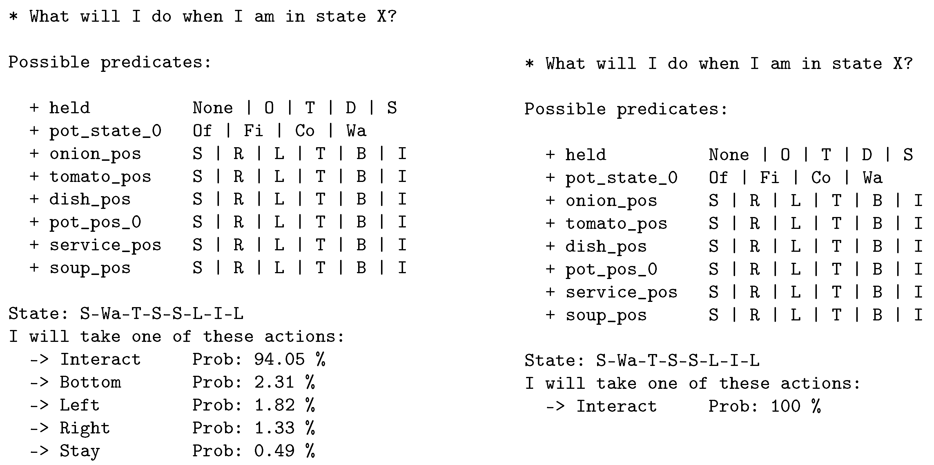
The following questions can be asked of a policy graph, which are a starting point to obtaining explanations on agent behaviour:

• What will you do when you are in state region X? (e.g., all states where pot_ state(Finished))
• When do you perform action a?
• Why did you not perform action a in state s?

Each of these questions can be answered with custom algorithms that leverage the probability distributions learnt by the policy graph. For our work, we borrow from and evolve upon the original conceptualisation found in [8] with some changes described in the following subsections. In Section 5.4, we open a discussion regarding the validity and the limitations of this approach.

5.1. What Will You Do When You Are in State Region X?

The answer to this question consists of aggregating the probabilities of possible actions in the policy graph from all the input states that the user wants to check. Let $PG=\langle V,E,A\rangle$ be the computed policy graph, $X\in S$ be the target state region, and dist: $\mathcal{P}\left(S\right)\times S⟼\mathbb{R}$ be a measure of distance between a discretised state and a state region in S. (This distance function can depend heavily on the environment and on the predicate set chosen. An in-depth analysis of possible functions is out of the scope of this paper, but it will be part of future work. For the sake of proof-of-concept, the distance function we have chosen for the work presented in this paper consists of: let $s\in S$ and $X=\{s_1,...\}\subseteq S$, we define dist$(X,s)={min}_{s_i\in X}$diff$(s_i,s)$, where diff is the function defined in Section 4. For example, this measure for the states in Figure 6 would be dist$(\left\{s_{left}\right\},s_{right})=4$ as only four predicates change value between them.) Very similarly to the possible courses of action of a surrogate agent defined in Section 4, there are three possible cases regarding the information available about the state region X.

• $|X\cap V|>0$: The policy graph generation algorithm has seen one or more states $s\in X$ during training, and it is likely that we can extract the probability of choosing among each of the accessible actions from them (this is only likely since a state s may have been visited very few times, and the estimation of probability may be little informed, in which case we would consider the other options in the list).
• $X\cap V=⌀$, but one or more similar states are found ($\exists s\in V:$dist$(X,s)<\epsilon ,\epsilon \in \mathbb{R}$): the policy graph has never seen any state in X, so we rely on a measure of similarity to another state to extrapolate (as in case 1).
• $X\cap V=⌀$ and no similar state is found: Returns a uniform probability distribution over all the actions.

A formal version of this procedure is shown in Algorithm 1.

Algorithm 1 What will you do when you are in state region X?

Input: Policy Graph $PG=\langle V,E,A\rangle$, Action Set A, Set of States X, Distance Threshold $\epsilon$ Output: Explanation of policy behaviour in X per action    $X^{\prime }\leftarrow X$   if  $X\cap V=⌀$then       $X^{\prime }\leftarrow \{v\in V|$dist$(X,v)=\underset{v^{\prime }\in V}{min}$dist$(X,v^{\prime })\}$▹ The set of states in V closest to X   end if   if  dist$(X,X^{\prime })>\epsilon$then       $\mathbf{P}\leftarrow Uniform\left(A\right);$   else       for all $a\in A$ do           $\mathbf{P}\left[a\right]\leftarrow \frac{{\sum }_{s\in X^{\prime }}P\left(a\right|s)P\left(s\right)}{{\sum }_{s\in X^{\prime }}P\left(s\right)}$       end for   end if   return  $\mathbf{P}$

For example, for the state region $\left\{\right\{$held(Service), pot_state(Waiting), onion_pos(Top), tomato_pos(Stay), dish_pos(Stay), pot_pos(Left), service_pos(Interact), soup_pos(Left)$\left\}\right\}$ (see Figure 7), the most probable action is to interact since the state shows us that the agent holds a soup and it is in front of the service.

5.2. When Do You Perform Action a?

The answer to such a question can be generated from an extensive list of all states that perform such an action (i.e., when is it the most likely?), as formalised in Algorithm 2.

For instance, when asking the policy graph of a trained agent for the Interact action, the list may include the state {held(Nothing), pot_state(Cooking), onion_pos(Left), tomato_pos(Stay), dish_pos(Interact), pot_pos(Left), service_pos(Right), soup_pos(Top)} (see Figure 8). There are three main predicates to analyse here: (1) the agent is empty-handed, (2) the pot is cooking, and (3) we are in an interact position with the dish pile. This results in picking up a plate, which seems reasonable given a plate is necessary to pick up soup from the pot once it finishes cooking.

Algorithm 2 When do you perform action a?

Input: Policy Graph $PG=\langle V,E,A\rangle$, Target Action a Output: Set of target states $S_{P{G}^a}$ where target a is the dominant action, Set of non-target states $S_{P{G}^{*a}}$   $S_{P{G}^a}\leftarrow \left\{\right\}$   $S_{P{G}^{*a}}\leftarrow \left\{\right\}$   for all  $s\in V$  do       $a^{*}\leftarrow \underset{a\in A}{argmax}P\left(a\right|s)$       if $a^{*}=a$ then           $S_{P{G}^a}\leftarrow S_{P{G}^a}\cup s;$       else           $S_{P{G}^{*a}}\leftarrow S_{P{G}^{*a}}\cup s;$       end if   end for   return  $S_{P{G}^a},S_{P{G}^{*a}}$

An intuitive improvement over this version would be finding which subset of satisfied predicates are sufficient to cause the action being picked. This would greatly reduce the complexity of analysis, given that instead of outputting a large number of states, we would find a small set of partial predicates.

5.3. Why Did You Not Perform Action a in State s?

This question is a non-trivial counterfactual question, regarding a transition: doing action a in a state s which potentially has never been sampled (hence the value in answering the question). To do so, Algorithm 3 finds the neighbouring states (i.e., states within a distance threshold in the metric space proposed in Section 5.1) and lists the difference in predicate sets between the regions where action a is performed and where it is not. Much like before, we distinguish between three cases depending on the characteristics of s:

• $s\in V$: The states within a distance threshold $\delta$ to s are gathered and filtered to those where action a is the most likely ($S_{P{G}^a}$). The output is the list of differences $\forall v\in S_{P{G}^a},preds\left(s\right)-preds\left(v\right)$. If $S_{P{G}^a}=⌀$, no explanation is given, and it is suggested to increase the threshold.
• $s\notin V$ but $\exists s^{\prime }\in V:$dist$(\left\{s\right\},s^{\prime })<\epsilon ,\epsilon \in \mathbb{R}$: the state $s^{\prime }$ substitutes s in the algorithm above.
• $s\notin V$ and no similar state is found: no explanation is given due to lack of information.

Algorithm 3 Why did you not perform action a in state $s_p$?

Input: Policy Graph $G=V,E$, Target Action a, Previous State $s_p$, Distance Threshold $D_{const}$ Output: Explanation of difference between current state and state region where $a_t$ is performed, explanation of where $a_t$ is performed locally.   $S_{{\pi }^a}\leftarrow \left\{\right\}$   $S_{{\pi }^{*a}}\leftarrow \left\{\right\}$   for all  $s\in \{v\in V\mid$dist$(\left\{v\right\},s_p)\le \epsilon \}$do       $a^{*}\leftarrow most\_frequent\_action\_executed\_from\left(s\right);$       if $a^{*}==a$ then           $S_{{\pi }^a}\leftarrow S_{{\pi }^a}\cup s;$       else           $S_{{\pi }^{*a}}\leftarrow S_{{\pi }^{*a}}\cup s;$       end if   end for   $expected\_region\leftarrow describe(S_{{\pi }^a},S_{{\pi }^{*a}},C);$   $current\_region\leftarrow describe(\left\{s_p\right\},S_{{\pi }^a},C);$   return  $diff(expected\_region,current\_region),expected\_region;$

As an example, consider the answer to “why the agent did not take the top action in state {held(Dish), pot_state(Cooking), onion_pos(Left), tomato_pos(Stay), dish_pos(Interact), pot_pos(Top), service_pos(Bottom), soup_pos(Left)}?”, as seen in Figure 9. This state is not part of the policy graph, whereas the one where dish_pos(Stay) indeed is (the difference being whether the dish pile is in the agent’s interact position (s) or south ($s^{\prime }$). The predominant action in state $s^{\prime }$ is going to the left. This algorithm’s output is the list of nearby states where the chosen action is top. For example, {held(Dish), pot_state(Cooking), onion_pos(Left), tomato_pos(Stay), dish_pos(Stay), pot_pos(Right), service_pos(Right), soup_pos(Top)}, where the nearest soup was on top. Seeing the difference, a human interpreter may understand that the agent has taken the action which brings him closer to the soup. The output of the algorithm itself is arguably not an explanation, but it gives information which could be useful in providing one.

5.4. Can We Rely on These Explanations?

As we mentioned in Section 1, one of the objectives of this project is to test if we can obtain valid explanations from an agent behaviour using the explainability method used in [9] in a multi-agent cooperative environment. In this section, we have seen some examples of the explanations given by our policy graphs.

We would like to emphasise the fact that not all the explanations given by the policy graph are so easy to interpret or understand at first sight. For instance, in Figure 9, we have seen that we asked the policy graph why the agent did not perform the Top action in the state {held(Dish), pot_state(Cooking), onion_pos(Left), tomato_pos(Stay), dish_pos(Interact), pot_pos(Top), service_pos(Bottom), soup_pos(Left)}. In this case, the algorithm answered that they would have chosen to go to the left, but the reason behind this decision is not so clear here, at least at first sight. We could elaborate hypotheses about the strategy that each agent was playing and maybe they could understand their decision. There is also the possibility that in this state, the agent is not choosing the more appropriate action. Although analysing these aspects in more depth is crucial for the objective of achieving better explainability, it is out of the scope of this paper, so we leave it for future work.

The policy graphs derived in the previous sections enable the generation of natural language explanations. In [8], the explanations are validated by comparing the sentences generated by the algorithm against sentences written by human experts. While this may be a valid qualitative approach for validation, it relies on expert availability and on the nature of the specific domain.

Even though sometimes the explanations given by the method are not as illustrative as we intended, at least we have an explanation. Namely, although at first glance we have not been able to draw too many conclusions, this method is explaining to us what has to happen for the agent to take said action. Therefore, it is one more tool to study and analyse the behaviour of these types of AI models. For all the reasons mentioned above, we can say we have met the goal of extracting useful explanations from the policy graph.

6. Validating the Policy Graph

To ensure that the policy graphs provide true explanations, we generate a policy graph for each Overcooked layout based on the trajectories of 1500 episodes on different seeds, and we build surrogate agents from them as explained in Section 4. In order to test these new surrogate agents, we run them through the environment for a total of 500 different fixed seeds and track the obtained rewards, the amount of previously unknown states encountered, the amount of served soups per episode and the mean log-likelihood $-\overline{l}=-\sum logP(s^{\prime },a|s)$ of the original’s trajectories for each policy graph.

In order to gauge the effect of cooperative predicates, we build four policy graphs per Overcooked layout, which are increasingly more expressive in relation to the state and actions of the agent’s partner. For each of the four policy graphs, we use a different subset of the 10 predicates defined in Section 4. We give these subsets of predicates the names D11 to D14 (

Table 3. Sets of predicates used to generate policy graphs. Note that held_partner and partner_zone are the only cooperative predicates in the sets.

	Single-Agent			Coop.
	held	pot_state	object_pos	held_partner	partner_zone
D11	X	X	X
D12	X	X	X	X
D13	X	X	X		X
D14	X	X	X	X	X

).

As we saw in Section 4, we are testing two different policy graph generation algorithms. Therefore, we have built two surrogate agents for each layout. We call an agent Greedy if its policy is generated from a greedy policy graph; analogously, we call an agent Stochastic if its policy is generated from a stochastic policy graph.

All experiment runs on the Overcooked environment have been performed using Python 3.7, PantheonRL v0.0.1 [23] and Overcooked-AI v0.0.1 (https://github.com/HumanCompatibleAI/overcooked_ai, accessed on 15 November 2023). All PPO agents have been trained with Stable Baselines 3 v1.7.0 [26], while the policy graphs have been generated with NetworkX v2.6.3 (https://networkx.org/, accessed on 15 November 2023).

• $S\in PG$: Picks an action using weights from the probability distribution in the PG.
• $S\notin PG$, but a similar state is found: Same as case 1 but using the similar state.
• $S\notin PG$ and a similar state is not found: Pick a random action.

Figure 10 shows the rewards obtained by the different surrogate agents. We can see that in the simple and unident_s scenarios, the greedy surrogate agents manage to consistently outperform the original ones while the stochastic ones do not. We can also see how in random1, the greedy agents are not able to function properly while the stochastic agents almost score as well as the originals. Note how the addition of the partner_zone predicate to an agent clearly improves its median score or makes it perform better more consistently in several cases. Examples include the greedy agents for simple, random3 and random0 and the stochastic agents for simple, random1 and random3. It also can be seen that although they may improve performance, in most layouts, it is not necessary to introduce cooperative predicates to explain the surrogate agents’ behaviour. In the random0 scenario, though, the agents need the predicate partner_zone to obtain good results.

Regarding the encounter of previously unknown states (

Table 4. Surrogate agent statistics. |PG| represents the size of the agent’s policy graph. NS means amount of new states encountered, %|PG| represents the amount of new states as a proportion of the size of the agent’s policy graph, and %steps indicates the percentage of steps during the evaluation runs that the agent spent in new state. $-\overline{l}$ is the negative log-likelihood. Note that a previously unknown state transition would make the log-likelihood go to Infinity, so instead we penalise it by $mi{n}_{PG}logP(s^{\prime },a|s)$.

				Greedy			Stochastic
		$-\overline{\mathit{l}}$	|PG|	NS	%|PG|	%steps	NS	%|PG|	%steps
simple	D11	880.1	475	0	0.0%	0.0%	70	14.7%	1.3%
	D12	996.2	884	2	0.2%	0.0%	75	8.5%	0.6%
	D13	1036.2	1045	5	0.5%	0.0%	94	9.0%	0.5%
	D14	1042.0	1734	5	0.3%	0.0%	135	7.8%	0.3%
random_1	D11	696.1	2663	2	0.1%	0.0%	197	7.4%	1.6%
	D12	731.4	5016	0	0.0%	0.0%	625	12.5%	3.2%
	D13	828.2	5256	0	0.0%	0.0%	530	10.1%	2.3%
	D14	827.8	8566	29	0.3%	0.3%	1260	14.7%	3.2%
random_3	D11	760.5	2195	31	1.4%	3.2%	177	8.1%	1.2%
	D12	787.1	3613	54	1.5%	1.4%	419	11.6%	1.4%
	D13	859.3	3536	92	2.6%	4.3%	595	16.8%	1.6%
	D14	878.6	5436	161	3.0%	2.1%	827	15.2%	1.3%
unident_s	D11	559.5	202	0	0.0%	0.0%	12	5.9%	0.2%
	D12	673.8	464	0	0.0%	0.0%	49	10.6%	0.1%
	D13	743.0	422	1	0.2%	0.0%	19	4.5%	0.0%
	D14	777.4	900	5	0.6%	0.0%	70	7.8%	0.1%
random0	D11	650.5	1793	3	0.2%	0.3%	133	7.4%	1.6%
	D12	693.6	3089	37	1.2%	30.6%	268	8.7%	2.1%
	D13	710.9	2696	6	0.2%	0.0%	181	6.7%	1.2%
	D14	745.5	4392	36	0.8%	0.3%	285	6.5%	1.7%

), we can see that most of the greedy surrogate agents achieve a very small amount of new states in relation to their policy graph’s size (i.e., already seen states) and spend a very little amount of steps in them in relation with the total evaluation time. An exception is random_3, for which it appears that there still was a notable amount of states to explore when building the policy graph. On the other hand, all the stochastic surrogate agents can consistently arrive at unexplored states to a higher degree than their greedy counterparts. This is to be expected, as the stochastic nature of the former inherently promotes exploration.

Also in Table 4, we can observe that the episode trajectories achieved by the original agents have a better mean log-likelihood with the D11 policy graphs than the others. This stems from the fact that the policy graphs built with D11 have a simpler world representation than those built with D12–D14, as D11 is the smallest subset of predicates in use. As a result, these policy graphs have less entropy.

To summarise, the stochastic policy graphs provide stable surrogate agents that mirror the original agent’s behaviour consistently. However, greedy policy graphs are a double-edged sword: their surrogate agents can act like distilled versions of the original’s behaviour that remove noise, or they can stop functioning because their deterministic nature did not capture fundamental parts of the original’s behaviour. Thus, stochastic policy graphs are the more reliable choice from an XRL point of view and should be the one used for producing explanations.

We have also seen that although there are scenarios where it is not necessary to introduce cooperative predicates to explain the agent’s behaviour, there are others—particularly those that promote the need for cooperation—where this information is crucial.

7. Conclusions

Explainability in Artificial Intelligence is a research area that has been rapidly growing in recent years due to the need to understand and justify the decisions made by AIs, especially in the field of RL. All the research made in this area can be key not only to study the quality of an agent’s decision but also to help people rely on AI, especially in situations where humans and machines have to cooperate, and it is becoming necessary to be able to give explanations about their decisions. There are already some proposals in the literature to provide them, and it is important to test their effectiveness in practice.

In this paper, we have presented the procedure and the experimental results of the first use case of an explainability method, based on the construction of a policy graph by discretising the state representation into predicates, into a cooperative MARL environment (Overcooked). We have proposed two different algorithms to generate the policy graph, and we have used them to generate explanations that, following [8], can be transformed into human language expressions. In principle, the quality of these explanations can be qualitatively validated by human experts with domain-specific knowledge. Our contribution to this respect is a quantitative validation of the generated policy graphs by applying a method previously employed into a single-agent environment (Cartpole) [9], automatically generating policies based on these explanations in order to build agents that represent their original behaviour. Finally, we have analysed the behaviour of agents following these new policies in terms of their explainability capabilities, depending on the environmental conditions, and we have shown that relevant predicates for cooperation become also important for the explanations when the environmental conditions influence the need for such cooperation.

The contributions presented in this paper are part of ongoing research, by testing among different environments, types of agent policy, and explainability methods. Therefore, several important points can be explored to complement and advance our work. For example, policy graphs are rarely complete, as seen in Section 6. It would be very interesting to be able to produce a domain-agnostic distance function that enables a reliable detection of similar states for different environments.

There should also be a more general and comprehensive analysis of the question-answering capabilities of policy graphs, as this can help with quantifying the understandability of the explanations produced. One way can be via the exploration and creation of new algorithms, adding to the ones explored in this paper, in order to attend to other modalities that the receivers of explanations might find important. Additionally, a more thorough study of when and why the policy graphs adjust better to the original agent, regardless of the specific domain—in terms of, for instance, whether the policy is greedy or stochastic, or what the relationship between each subset of predicates and the performance is.

Finally, other environments should be explored. Specifically, Overcooked-AI requires cooperation in some layouts but this cooperation is not explicitly reflected in the policy but emerging from the behaviour. It would be interesting to explore an application of policy graphs in an environment where there are explicit mechanisms such as communication or cooperative planning. In competitive or mixed-motive environments, such as StarCraft II [27], Neural MMO [28], Google Research Football (https://github.com/google-research/football, accessed on 5 December 2023), or Multi-Agent Particle [29], there also exists potential in using policy graphs to create a model of the behaviour of opponent agents based on observations. The resulting graph could be leveraged by an agent using Graph Neural Networks (GNNs) [30] to change its own behaviour with the purpose of increasing performance against specific strategies previously encountered.