Abstract
In the field of mining robot maintenance, in order to enhance the research on predictive modeling, we introduce the LODS model (long short-term memory network (LSTM) optimized deep fusion neural network (DFNN) with spatiotemporal attention network (STAN)). Traditional models have shortcomings in handling the long-term dependencies of time series data and mining the complexity of spatiotemporal information in the field of mine maintenance. The LODS model integrates the advantages of LSTM, DFNN and STAN, providing a comprehensive method for effective feature extraction and prediction. Through experimental evaluation on multiple data sets, the experimental results show that the LODS model achieves more accurate predictions, compared with traditional models and optimization strategies, and achieves significant reductions in MAE, MAPE, RMSE and MSE of 15.76, 5.59, 2.02 and 11.96, respectively, as well as significant reductions in the number of parameters and computational complexity. It also achieves higher efficiency in terms of the inference time and training time. The LODS model performs well in all the evaluation indexes and has significant advantages; thus, it can provide reliable support for the equipment failure prediction of the mine maintenance robot.
1. Introduction
In the field of industrial automation, intelligent mine maintenance robots are playing an increasingly critical role. Faced with the extreme characteristics of the mining environment and the high complexity of maintaining equipment, they must cope with the sudden and unpredictable nature of equipment failures [1]. The characteristics of equipment failures increase the difficulty of maintenance work, forcing us to consider developing advanced predictive models to effectively address them.
Deep learning, as a powerful data analysis and predictive modeling technology, has demonstrated its outstanding capabilities in multiple fields. In particular, its performance in feature learning and pattern recognition has proven to be beneficial in mining potential information in data, thereby improving the accuracy and efficiency of prediction [2]. However, there are several challenges that need to be overcome to successfully apply deep learning technology to the predictive maintenance of mine maintenance robots. The data generated by these robots often have complex multi-modal timing characteristics, including but not limited to sensor data, images and sounds [3]. The traditional method that uses single-modal data as the main body of analysis fails to comprehensively examine and understand the operating status of the equipment, making it difficult to meet the needs of practical applications [4].
With the aid of deep learning technology, we expect to overcome the limitations of current methods and achieve more accurate and reliable equipment failure predictions. The high adaptability and autonomous learning capabilities of deep learning make it a powerful tool to solve multi-modal time series data problems [5]. By further improving and adapting the deep learning model, we expect to achieve a qualitative leap forward in the field of fault prediction for mine maintenance robots.
Most current research focuses on the processing of single-modal data and ignores the importance of the comprehensive analysis of multi-modal data. At the same time, the characteristics of long-term dependencies in time series data and the complexity of spatiotemporal data pose additional challenges to predictive modeling. This study will provide a comprehensive evaluation of several currently widely used deep learning models, aiming to explore their potential application scenarios and challenges in the field of mine robot maintenance and provide a theoretical basis for the model construction in this study.
As a powerful image processing tool in deep learning, the convolutional neural network (CNN) can effectively capture the spatial hierarchical features of images through its stacked convolutional layers and pooling layers [6]. This means that the CNN shows great potential in image analysis tasks in the field of mining robot maintenance, especially in identifying tiny cracks, corrosion or other forms of defects on the surfaces of equipment [7]. However, in the face of analysis tasks involving complex multi-modal time series data, such as processing images, sound and sensor data simultaneously, the CNN needs to integrate additional structures for effective information fusion [8].
The temporal convolutional network (TCN) adopts a one-dimensional convolution structure [9]. Its main advantage is to effectively learn the local features of temporal data and it has excellent short-term dependency capture capabilities [10]. The TCN has great application potential in mine maintenance diagnosis. It can analyze time series data generated by sensors to monitor and predict equipment performance [11]. However, the TCN may not be effective in capturing long-term dependencies.
Graph convolutional networks (GCNs) are specifically designed to process graph data and are capable of identifying complex patterns in graph structures [12]. In mining robot maintenance, GCNs can reveal the interactions and dependencies between equipment, providing a more comprehensive system perspective for prediction [13]. However, GCNs face challenges in terms of computational efficiency and scalability when facing large device networks [14].
The Transformer model, with its self-attention mechanism as its core, provides a new solution for the capturing of long-distance dependencies of sequences [15]. When applied to mining robot maintenance, the Transformer model is able to process time series data from different modalities and provide accurate predictions by capturing inherent global dependencies [16]. However, Transformer’s high computing requirements limit its deployment in resource-constrained practical application scenarios [17].
Although deep learning models such as CNN, TCN, GCN and Transformer have achieved certain results in the field of mine robot maintenance, they still have shortcomings in processing multi-modal time series data and long-term dependencies in special environments. Traditional CNNs may face difficulties in information fusion [18], The TCN may have certain challenges in modeling long-term dependencies [19], the GCN may have computational efficiency issues in large-scale graph data processing [20], and Transformer may face some computational complexity issues [21].
Based on the shortcomings of the above methods, we propose the LODS model (LSTM-optimized DFNN with STAN). The LODS model uses the long short-term memory network (LSTM) as an optimization module and integrates a deep fusion neural network (DFNN) and spatiotemporal attention network (STAN) through synergy. The DFNN is responsible for processing multi-modal data, while the STAN focuses on the characteristics of spatiotemporal data. The LSTM optimization module helps to integrate the two aspects of information and is especially suitable for processing time series data, improving the accuracy of the model’s time series prediction of equipment failures. The LODS model provides a comprehensive and efficient deep learning solution for the field of mining robot maintenance, enabling us to more comprehensively understand the equipment status and improve the accuracy and reliability of fault prediction. Its advantages are reflected in the comprehensive analysis of multi-modal time series data, spatiotemporal data modeling and long-term dependency processing, providing more reliable decision support for mine maintenance work. By introducing the LSTM optimization module, the model achieves better information collaboration between different modalities and data characteristics, providing an innovative solution for the equipment failure prediction of mine maintenance robots.
The main contributions of this study are as follows:
- The pioneering nature of the LODS model: This study proposes the LODS model, which is an innovative multi-modal time series data analysis framework that combines a deep fusion neural network (DFNN), spatiotemporal attention network (STAN) and long short-term memory network (LSTM). It provides a new modeling method for the field of mine robot maintenance.
- Multi-modal data fusion: The LODS model uses DFNN to deeply integrate various data sources, which enhances the model’s understanding of the equipment status and provides more comprehensive information support for fault prevention.
- Spatiotemporal dependency optimization: The STAN module is used to enhance the capture of key spatiotemporal data, and the LSTM module is used to improve the long-term dependency modeling capabilities, greatly improving the accuracy of equipment failure prediction.
In the following sections, we will structure our discussion as follows. Section 2 will introduce the method in depth and reveal the core construction and design principles of the LODS model. Section 3 will focus on the experimental settings and details in order to reproduce the experiment. Section 4 will introduce the experimental results in detail to show the performance of the LODS model in different data sets and scenarios. Finally, Section 5 discusses and summarizes the full text.
2. Methods
2.1. Overview of Our Network
The LODS model (LSTM-optimized DFNN with STAN) that we propose aims to provide a comprehensive and efficient deep learning solution for mining robot equipment failure prediction. The core construction of the LODS model includes three key components: DFNN, STAN and LSTM.
The DFNN is responsible for processing multi-modal data, including sensor data, images and sounds, etc. Through the deep fusion layer, the DFNN effectively fuses the information processed in different branches to achieve a comprehensive understanding of the multi-modal information. The purpose of this section is to provide more comprehensive device information and promote a comprehensive understanding of the device’s health status. The STAN module uses an attention mechanism to focus on the spatiotemporal data characteristics in the mining environment. This helps the network to better focus on critical moments and areas and increase its sensitivity to changes in the device status. The role of the STAN in the mine maintenance environment is to capture the complexity of the spatiotemporal data and enhance the network’s understanding of the entire system status. The LSTM serves as an optimization module and integrates the output of the DFNN and STAN. It is particularly useful in capturing long-term dependencies in time series data. Through the introduction of the LSTM, we optimize the model’s timing prediction accuracy for equipment failures and improve the performance of the overall model.
The network construction process of the LODS model is divided into the following steps. First, we design the DFNN network branch to process multi-modal data, including images, sensor data and sounds. Each branch contains an adaptive hierarchy to extract features of a specific data type. Then, the STAN network branch is designed, which is used to process spatiotemporal data and uses the attention mechanism to capture information at key moments and regions. This branch models multi-modal data in the spatiotemporal dimension. Then, we perform information fusion, using the deep fusion layer to fuse the information of the DFNN and STAN branches to form a global, multi-modal feature representation. Finally, the LSTM is introduced as an optimization module to integrate the fused feature representation to better capture the long-term dependencies in the time series data and improve the time series prediction performance of the model.
The overall model structure diagram is shown in Figure 1.
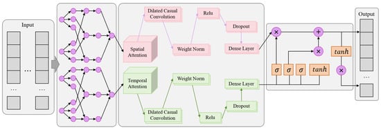
Figure 1.
Overall flow chart of the model.
The running process of the LODS model is shown in Algorithm 1.
| Algorithm 1: LODS Training |
| 1: Input: Training data from C-MAPSS, SECOM, PHM08, Tennessee Eastman 2: Output: Trained parameters of the LODS model 3: Initialize LSTM parameters , DFNN parameters , STAN parameters 4: Initialize optimizer parameters 5: for each training epoch do 6: for each batch in do 7: Sample a batch of multi-modal time series data 8: Extract features using DFNN: 9: Extract spatiotemporal features using STAN: 10: Concatenate DFNN and STAN features: 11: Apply LSTM for sequence modeling: 12: Compute loss: 13: Backpropagate gradients and update LSTM, DFNN, STAN parameters 14: Update optimizer parameters using backpropagation: 15: end for 16: end for 17: return Trained parameters: |
In this model, for the “Input” section, the input data of our model include three main types: one is the sensor data, which are the time sequence data from different sensors of mine robots and may include the numerical sequences of temperature, pressure, vibration and other indicators; the other is image data, which refer to the images of the mine robot’s working environment or continuous camera frame sequences, used to capture the visual state information of the device; the other is sound data for the acoustic signals captured during the robot’s operation, which can help to detect the abnormal noise of the device to assist in fault prediction. The LODS model uses the DFNN network to process the above multi-modal data and performs deep fusion. For the “Output” section, the data type output by the model is the prediction of the potential failure of the mine robot equipment. Specifically, the output data can be qualitatively defined as probability values or classification results, meaning that every possible failure type will be assigned a predicted probability by our model. Further, these prediction results can help the maintenance team to make timely repair or maintenance decisions.
2.2. Deep Fusion Neural Network
The deep fusion neural network (DFNN) is a deep learning model focused on processing multi-modal data. The basic principle is to process different types of data, such as sensor data, images and sounds, in different branches of the network, and then effectively fuse the information of these branches through a deep fusion layer to improve the prediction performance for equipment failures [22]. The main purpose of the DFNN is to achieve the organic integration of different data types in complex multi-modal data scenarios to more comprehensively understand the status of the system [23].
In the application of mine robot maintenance, the DFNN model shows its powerful comprehensive data processing capability, especially in processing multi-modal data. Unlike traditional methods, the DFNN model not only deals with a single form of data, such as the readout of the sensor, but also can integrate and analyze multi-modal data from different sources, including but not limited to high-resolution images, complex sound signals and multi-dimensional sensor data. For example, when monitoring the health of key maintenance components such as hydraulic arms, the DFNN can use data from vibration sensors, acoustic monitoring equipment and visual detection systems, which are subtle signals that may be missed by a single data source.
The internal architecture of the DFNN is specifically designed with a deep fusion layer, which is tailored to the characteristics of different data modalities and the optimal way to extract features. For example, our model uses convolutional neural network branches to process image data to identify visual patterns and texture abnormalities, while using recurrent neural network branches to process sound signals to capture temporal dependence and periodicity characteristics. Using the features obtained by these branches, the deep fusion layer of the DFNN uses innovative fusion algorithms to effectively combine them and establish meaningful associations between different data streams.
In the LODS model constructed in this work, the DFNN undertakes the task of processing multi-modal data. Its function is to organically integrate information from different branches through a deep fusion layer to form a global feature representation. This fusion of multi-modal information enables the model to more comprehensively understand the working status of the equipment, providing a more accurate basis for the prediction of equipment failures. The function of the DFNN in the overall model is to provide the efficient processing of different data types and generate more informative feature representations through fusion, thereby providing strong support for subsequent spatiotemporal data modeling and the optimization of long-term dependencies. Its importance lies in its ability to provide global and multi-dimensional device information for the LODS model, making a key contribution to improving the performance of the overall model.
The structure diagram of the DFNN model is shown in Figure 2.
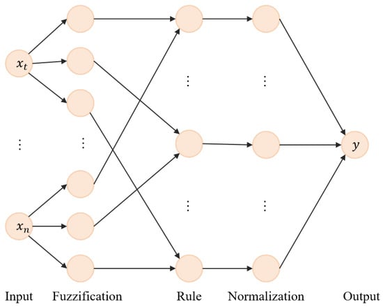
Figure 2.
Flow chart of the DFNN model.
The main formula of the DFNN is as follows:
where is the update gate at time t, is the sigmoid activation function, and are weight matrices for the input and hidden state, is the input at time t, is the hidden state at time , and is the bias vector for the update gate.
where is the reset gate at time t, is the sigmoid activation function, and are weight matrices for the input and hidden state, is the input at time t, is the hidden state at time , and is the bias vector for the reset gate.
where is the candidate hidden state at time t, tanh is the hyperbolic tangent activation function, and are weight matrices for the input and hidden state, is the input at time t, is the reset gate at time t, is the hidden state at time , and is the bias vector for the candidate hidden state.
where is the hidden state at time t, is the update gate at time t, and ⊙ denotes element-wise multiplication.
where is the predicted class at time t, and is the argmax function that outputs the index of the maximum element.
2.3. Spatiotemporal Attention Network
The spatiotemporal attention network (STAN) is a deep learning model focused on processing spatiotemporal data [24]. The basic principle is to use the attention mechanism to enable the network to better focus on key moments and areas, thereby enhancing the modeling ability for spatiotemporal data [25]. The main purpose of the STAN is to capture temporal and spatial relationships in the data and it is suitable for data scenarios where time and space characteristics need to be considered.
In the practice of mine robot maintenance, there are complex time sequence data and location correlations. By introducing an attention mechanism, this model not only accurately calibrates key time points, but also identifies areas with a significant impact on the performance of the device. The STAN model is significantly better in capturing the intrinsic connections between spatiotemporal data than traditional deep learning methods. Through the built-in spatial and temporal attention component, the model can identify the patterns that have a significant impact on the running state of the entire mine machine in the continuous data flow. For example, when predicting conveyor belt wear, the STAN uses its spatiotemporal attention mechanism to pinpoint abnormal wear patterns occurring in specific operating conditions, thus providing decision support for early maintenance and replacement. The STAN model utilizes the attention scoring mechanism to prioritize the data regions that are most important for the current prediction target. In practical cases, when analyzing noise data generated by multiple sensors, it can distinguish abnormal sounds generated by equipment failures and distinguish them from background ambient noise, thus improving the fault detection rate and reducing false positives. The flexibility of the STAN is also reflected in its ability to process spatiotemporal data in different mining environments and equipment. For example, when monitoring the navigation system of a mine robot, the STAN is able to adapt to different terrain and obstacle configurations and optimize the path planning by analyzing the evolution of spatiotemporal data.
In the LODS model, the function of the STAN module is to model spatiotemporal data and enhance the understanding of the entire system state. Due to the complexity of spatiotemporal relationships in the mining environment, the introduction of STAN helps the network to better focus on critical moments and areas and improves its sensitivity to changes in equipment status. Its importance lies in the ability to provide the overall model with effective modeling capabilities for spatiotemporal data, thereby providing more accurate and comprehensive support for the prediction of equipment failures. In the equipment failure prediction of mine maintenance robots, the contribution of the STAN module not only improves the performance of the model but also strengthens the ability to adapt to the complexity of the mine environment.
The structure diagram of the STAN model is shown in Figure 3.
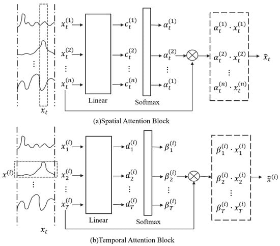
Figure 3.
Flow chart of the spatiotemporal attention network model.
The main formula of the STAN model is as follows:
where Q is the query matrix, K is the key matrix, V is the value matrix, X is the input matrix, and , , are learnable weight matrices.
where is the attention mechanism, is the softmax function, and is the dimension of the key vectors.
where is the multi-head attention, , , and is the output weight matrix.
where is the residual connection. is any of the sub-layers.
2.4. Long Short-Term Memory
The long short-term memory network (LSTM) is a variant of the recurrent neural network (RNN) with long short-term memory capabilities. The basic principle is that by introducing gate structures (forgetting gates, input gates and output gates), the LSTM model can better capture the long-term dependencies in time series data and effectively avoid the vanishing gradient problem [26]. The main use of LSTM is to process time series data, especially in scenarios where long-term dependencies need to be captured, such as speech recognition, text generation, etc. [27].
LSTM demonstrates its profound value in mine robot maintenance tasks, especially when processing and analyzing time series data collected by monitoring equipment. Mine robots usually operate in extreme and unpredictable environments; the data collected reflect the operating state of the robot’s systems, and these data show complex temporal characteristics. The LSTM model is suitable for such application scenarios, firstly, because the gating mechanism of LSTM is particularly suitable for analyzing the time series recorded by robotic sensors. In the mine environment, robotic components (e.g., drill bits, loading arms, delivery systems) may gradually experience subtle performance degradation, which show long-term trends in temporal data. By identifying these long-term dependencies, the LSTM can alert them to potential failures early, leaving more time for maintenance teams to respond. Second, in practice, LSTM has significant advantages over traditional RNN models in handling the stability and accuracy of long time series. This advantage is attributed to the gate structure in its design, which can effectively prevent the gradient disappearance or explosion problem and ensure the training stability. For mining robots, this means that the model can be used to track and analyze changes in its key operational parameters, allowing an accurate assessment of the robot’s long-term health. In addition, due to the inherent timing characteristics of the mine robot maintenance data, the LSTM model provides a more accurate and reliable prediction tool. By modeling the timing changes in device status, LSTM helps to develop maintenance plans and preventive maintenance strategies, reduce unexpected downtime and extend the operating life of the robot.
In the LODS model, the function of the LSTM module as an optimization module is to integrate the output of the DFNN and STAN branches to enhance the overall model’s ability to process time series data. By introducing LSTM, we can better capture the long-term dependencies of equipment state changes and improve the accuracy of the model in time series prediction. Its importance lies in providing the overall model with optimized support for time series data. By effectively integrating information from different branches, the model’s sensitivity and expressive ability regarding changes in equipment failure time series are improved. In the field of mining robot maintenance, the introduction of the LSTM module strengthens the model’s performance in processing equipment failure time series data, providing important support for the reliability of the entire prediction model.
The structure diagram of the LSTM model is shown in Figure 4.
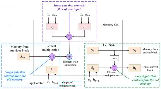
Figure 4.
Flow chart of the LSTM model.
The main formula of the attention mechanism is as follows:
where is the forget gate output at time t, is the weight matrix for the forget gate, is the hidden state from the previous time step, is the input at time t, is the bias vector for the forget gate, and is the sigmoid activation function.
where is the input gate output at time t, is the weight matrix for the input gate, and is the bias vector for the input gate.
where is the cell candidate at time t, is the weight matrix for the cell candidate, is the bias vector for the cell candidate, and tanh is the hyperbolic tangent activation function.
where is the cell state at time t, and ⊙ is the element-wise multiplication (Hadamard product).
where is the output gate output at time t, is the weight matrix for the output gate, and is the bias vector for the output gate.
where is the hidden state at time t.
3. Experiment
3.1. Experimental Environment
- Hardware Environment. The hardware environment used in the experiments consists of a high-performance computing server equipped with an AMD Ryzen Threadripper 3990X @ 3.70 GHz CPU and 1 TB RAM, along with 6 Nvidia GeForce RTX 3090 24 GB GPUs. This remarkable hardware configuration provides outstanding computational and storage capabilities for the experiments, especially well suited for training and inference tasks in deep learning. It effectively accelerates the model training process, ensuring efficient experimentation and rapid convergence.
- Software Environment. In this study, we utilized Python and PyTorch to implement our research work. Python, serving as the primary programming language, provided us with a flexible development environment. PyTorch, as the main deep learning framework, offered powerful tools for model construction and training. Leveraging PyTorch’s computational capabilities and automatic differentiation functionality, we were able to efficiently develop, optimize, and train our models, thereby achieving better results in the experiments.
3.2. Experimental Data Sets
In order to obtain comprehensive and representative experimental results, we selected four different data sets, including the C-MAPSS data set, SECOM Manufacturing Data, PHM08 Challenge Data and Tennessee Eastman Process Simulation Data.
The C-MAPSS Data Set is a classic data set used for aviation engine health monitoring, including multiple different types of engines. Each engine is equipped with multiple sensors, providing rich timing data [28]. This data set is widely used in the aviation field, providing complex and diverse engine operating states for the model and helping to verify the performance of the LODS model in complex environments. In this study, we selected engine data similar to the mine equipment sensor configuration to meet the fault prediction requirements of the LODS model in the mine-specific environment.
SECOM Manufacturing Data comes from the semiconductor manufacturing industry. It contains a range of sensor data from the semiconductor production process, covering both functioning and defective products [29]. The main characteristic of SECOM Manufacturing Data lies in its ability to capture diverse issues in the manufacturing process, providing the LODS model with training data that are closer to actual application scenarios. In this experiment, the features related to the fault detection in the production process of the mine robot were extracted, and the model was adjusted to accurately identify the unique fault signal of the mine robot.
PHM08 Challenge Data is a data set from the PHM community, specifically designed for mechanical system health prediction [30]. This data set contains sensor data from multiple devices and is complex and challenging. The use of PHM08 Challenge Data aims to test the LODS model’s ability to process the multi-source data of mechanical systems and its performance in challenging environments. This data set is used to evaluate and optimize the prediction accuracy of the LODS model under high load conditions by simulating the high load during the mine machine operation and its impact on the health state of the equipment.
Tennessee Eastman Process Simulation Data is an extensively researched chemical process simulation data set. This data set simulates the operation of a chemical plant and contains simulated sensor data under normal and fault operating conditions [31]. By using this data set, we aim to verify the robustness and reliability of the LODS model in handling complex failure prediction tasks in chemical processes. This data set is used to simulate the chemical factors that may affect the health of the robot equipment in the mine environment, and to test and verify the failure prediction model for this special scenario.
3.3. Experimental Setup and Details
In this paper, the LODS model (LSTM-optimized DFNN with STAN) model is constructed to meet the challenge of the fault prediction of mine maintenance robot equipment. To ensure the accuracy and reproducibility of the experiment, by thoroughly considering the design and details of the experiment, the specific experimental settings are detailed below.
Step 1: Data set preparation
- Data cleaning: In this paper, the features with more than 5% missing values are set as the objects to be processed, and the mean filling method is used for processing.
- Data standardization: This paper adopts the standard deviation standardization method to map the values of all features to the standard normal distribution with mean 0 and standard deviation 1.
- Data split: 70% of the data in the experiment are used for training, 20% for validation and 10% for testing. Random sampling is used to ensure the stochasticity and representativeness of the data set.
Step 2: Model training
- Network parameter setting: The initial learning rate is 0.001, the batch size is 64, and 150 rounds of iterative training are conducted.
- Model architecture design: The DFNN is responsible for processing multi-modal data, the STAN focuses on spatial and temporal relations and LSTM serves as an optimization module to integrate the output of both. Three branches are included in the DFNN that process sensor data, images and sound information. The STAN uses a three-layer attentional structure to model the relevance of data in spatiotemporal dimensions. The number of hidden cells of the LSTM was set to 128 to ensure that it effectively captured the long-term dependencies in the temporal data.
- Model training process: A stochastic gradient descent (SGD) optimizer was used, combined with a learning rate decay mechanism. During the training process, training was stopped to avoid overfitting when 10 consecutive rounds of validation set loss no longer decreased. Moreover, batch normalization and dropout were used to improve the robustness and generalization of the model.
Step 3: Model validation and tuning
- Cross-validation: The experiment uses k-fold cross-validation to divide the data set into k mutually exclusive subsets. Moreover, k = 10, to balance the computational cost and the accuracy of the performance evaluation.
- Model fine-tuning: During the fine-tuning process, we focus on the model hyperparameters such as the learning rate and batch size, as well as the details of the network structure. By systematically using different hyperparameter combinations, we chose the parameter settings to achieve the best performance on the validation set. To prevent overfitting, we also used regularization techniques to limit the complexity of the model.
Step 4: Ablation experiment
During the experiments in this paper, a series of ablation experiments were designed to investigate the impact of the various components of the LODS model on model performance. Remove experiments for each component were performed to assess its contribution to the overall model performance.
- Removing LSTM: This set of experiments removed the LSTM components from the overall LODS model and built the model using only the DFNN and STAN. The number of hidden cells in LSTM was set to 50 with a learning rate of 0.001.
- Remove STAN: This set of experiments removed STAN components from LODS and modeled only using the DFNN and LSTM. The number of attention heads in STAN was 4 with a learning rate of 0.002.
- Removing DFNN: This set of experiments retained the LSTM and STAN and removed the DFNN. The number of convolution kernels for DFNN was set to 16, with a learning rate of 0.001.
- Overall model LODS: In the full model, the LSTM, STAN and DFNN work together to comprehensively utilize temporal data, spatial–temporal relationships and multi-modal information. The number of hidden cells in LSTM is 100, the number of the heads of attention in STAN is 8, and the number of convolution kernels in the DFNN is 32, with an overall learning rate of 0.001.
Step 5: Comparative Analysis
In the experiments presented in this paper, comparison experiments were also designed, focusing on the optimization strategy, selecting Adam, Bayesian and PSO as comparison objects, and performing the performance comparison with LSTM.
- Adam vs. LSTM: In this comparison experiment, the learning rate of Adam was 0.001, and the number of hidden cells of LSTM was 100.
- Bayesian vs. LSTM: In this comparison experiment, the default settings of the Bayesian optimization strategy were adopted, and the number of hidden cells of LSTM was set to 100.
- PSO vs. LSTM: In this comparison experiment, the number of iterations of PSO was set to 50, the population size was set to 20, and the number of hidden cells of LSTM was set to 100.
Step 6: Model Evaluation In this study, we conducted a comprehensive and detailed evaluation of the LODS model, focusing on the two core dimensions of accuracy and efficiency.
- The accuracy of the model’s prediction ability is assessed using the following evaluation metrics: Mean Absolute Error (MAE), Mean Absolute Percentage Error (MAPE), Root Mean Square Error (RMSE) and Mean Square Error (MSE). A lower MAE value indicates greater accuracy in the model’s predictions. A low MAPE value indicates small errors and high prediction accuracy. RMSE permits a more stringent evaluation of the accuracy of the model by giving greater weight to larger errors. MSE is a key indicator in evaluating the model prediction performance in regression analysis.
- The efficiency of the model is evaluated using the following indicators: parameters, floating-point operations (FLOPs), inference time and training time. Models with fewer parameters are generally considered more efficient and concise. Lower FLOPs means that the model has a smaller demand for computing resources and has higher computing efficiency. The inference time directly reflects the real-time nature and response speed of the model. Training time measures the total time that it takes the model to complete the learning process during the training phase.
4. Results
We performed a comprehensive comparison of the LODS model against six alternative models across four distinct data sets. The evaluation incorporated several metrics, including the Mean Absolute Error (MAE), Mean Absolute Percentage Error (MAPE), Root Mean Square Error (RMSE) and Mean Square Error (MSE), alongside additional indicators, as detailed in Table 1. On the C-MAPSS data set, compared with other models, the LODS model achieved significant reductions in MAE, MAPE, RMSE and MSE, which were 15.76, 5.59, 2.02 and 11.96, respectively. This shows that the LODS model predicts equipment failures more accurately on the C-MAPSS data set. On the three data sets of SECOM Manufacturing Data, PHM08 Challenge Data and Tennessee Eastman Process Simulation Data, the LODS model also performed well. Compared with other models, it achieved lower MAE, MAPE, RMSE and MSE values, further proving its superiority on multiple data sets. It is particularly worth noting that, compared with the classic model mentioned earlier, the LODS model has achieved significant improvements in various indicators. This shows that the LODS model can better adapt to the complex multi-modal time series data of mine maintenance robots and improve the accuracy and reliability of equipment failure prediction. Comparing all data results, the LODS model performs well in all evaluation indicators and has significant advantages in predicting equipment failure in mine maintenance robots.

Table 1.
Performance comparison across models Using varied data sets.
Figure 5 visually presents the excellent performance of the LODS model in various performance indicators. It can be clearly observed from the figure that the LODS model has significant advantages over other models in indicators such as MAE, MAPE, RMSE and MSE.
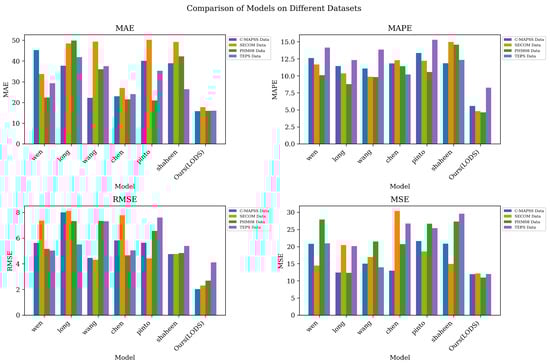
Figure 5.
Model accuracy verification comparison chart of different indicators of different models.
As shown in Table 2, we compared the LODS model with six other models on four different data sets, using metrics such as the model parameter volume, computational complexity (FLOPs), inference time and training time to evaluate the model performance. On the C-MAPSS data set, the parameter amount, computational complexity, inference time and training time of the LODS model are 337.64 M, 3.54 G, 5.37 ms and 325.19 s, respectively. Compared with other models, the LODS model has achieved significant reductions in parameter volume and computational complexity, while also achieving higher efficiency in terms of inference time and training time. The LODS model also performed well on the three data sets of SECOM Manufacturing Data, PHM08 Challenge Data and Tennessee Eastman Process Simulation Data. Specifically, the number of parameters, computational complexity, inference time and training time of the LODS model on these three data sets are significantly better than those of other models, further proving its efficiency on multiple data sets. Of particular note is that the LODS model performs well in terms of computational complexity and has lower FLOPs than other models, indicating that it improves the prediction performance while reducing the computational costs. Overall, the LODS model performed well in all evaluation indicators, not only achieving significant improvements in prediction performance, but also achieving higher efficiency in terms of model parameters and computational complexity.
Table 2.
Model efficiency verification and comparison of different indicators of different data sets.
Figure 6 further visually presents the performance comparison of the LODS model on different data sets. By observing the chart, it can be clearly found that the LODS model performs well on multiple data sets, such as C-MAPSS, SECOM Manufacturing Data, PHM08 Challenge Data and Tennessee Eastman Process Simulation Data, demonstrating its performance in different mine maintenance robot task scenarios. It shows universality and robustness.
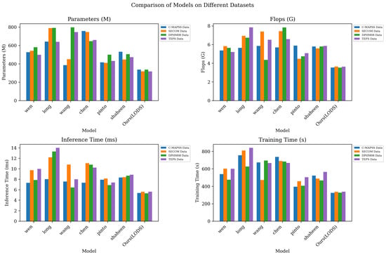
Figure 6.
Model efficiency verification comparison chart of different indicators of different models.
As shown in Table 3, we conducted a series of ablation experiments to remove the LSTM, STAN and DFNN components in the LODS model, as well as the comparison of the overall model. The experimental results after removing LSTM (DFNN + STAN) show MAEs of 49.73 and 36.86 on C-MAPSS and PHM08 Challenge Data, respectively, which are significantly higher than the 10.52 and 19.84 of the overall LODS model. This shows that LSTM plays a key role in the model performance when dealing with long-term dependencies in time series data. The experimental results after removing the STAN (DFNN + LSTM) on the Tennessee Eastman Process Simulation Data show an MAPE of 10.89, which is significantly higher than the 5.54 of the LODS model. This shows that the STAN plays a positive role in improving the model performance when considering spatiotemporal relationships. The experimental results after removing the DFNN (STAN + LSTM) show RMSEs of 6.76 and 5.93 on C-MAPSS and PHM08 Challenge Data, respectively, which are higher than the 2.98 and 2.23 of the LODS model. This implies the importance of the DFNN in multi-modal information fusion, especially when processing data such as images. The overall LODS model achieves better performance on all data sets relative to any single-component model. On C-MAPSS and PHM08 Challenge Data, the MAE of LODS is only 10.52 and 19.84, respectively, further verifying its excellent performance in mine maintenance robot tasks.
Table 3.
Ablation experiments on the LODS model using different data sets.
Figure 7 shows the comparison of the different models in different performance indicators, which further confirms the significant comprehensive performance advantage of the LODS model compared with each single-component model in the ablation experiment.
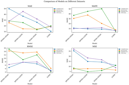
Figure 7.
Ablation experiments on the LODS model.
As shown in Table 4, we conducted a series of comparative experiments, using Adam, Bayesian and PSO as comparison objects and comparing their performance with that of LSTM. The following conclusions can be drawn from the data in the table. For the Adam vs. LSTM experiment, on C-MAPSS and PHM08 Challenge Data, the LODS model is significantly better than the Adam optimization strategy in indicators such as MAE and RMSE. Especially on C-MAPSS, the MAE of LODS is only 10.52, while that of Adam is 374.35, which shows the excellent performance of LODS in fault prediction tasks. For the Bayesian vs. LSTM experiment, the LODS model achieved better performance on all data sets. Compared with the Bayesian optimization strategy, it performed better in indicators such as MAPE and RMSE. For example, on the PHM08 Challenge Data, the MAPE of LODS is 4.48, while that of the Bayesian is 262.26, further verifying the superiority of LODS. For the PSO vs. LSTM experiment, on C-MAPSS and PHM08 Challenge Data, the LODS model is significantly better than the PSO optimization strategy in indicators such as MAE and RMSE. Especially on C-MAPSS, the MAE of LODS is 10.52, while that of PSO is 312.10, indicating that LODS is more reliable in fault prediction tasks. Overall, the LODS model has better performance than the optimization strategies in various comparative experiments.
Table 4.
Ablation experiments on the LSTM model using different data sets.
Figure 8 visualizes the contents of the table and shows the comparison of the different performance indicators of each model through intuitive charts, further proving the superior performance of the LODS model in mining robot maintenance tasks.
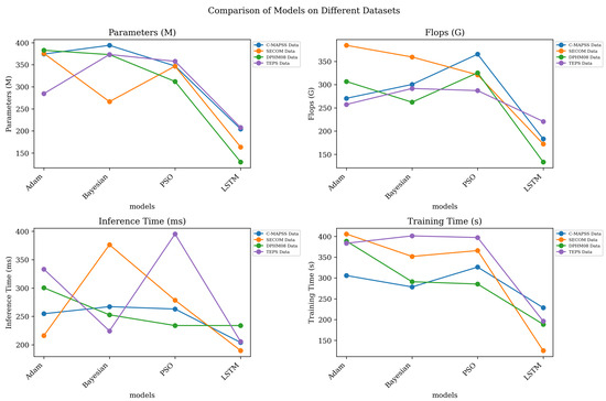
Figure 8.
Ablation experiments on the LSTM model.
5. Discussion
In this study, we propose an innovative LODS model designed to improve the accuracy of the predictive modeling of mine robots when performing maintenance tasks through an in-depth analysis of multi-modal temporal data. The model combines the advantages of the long short-term memory network (LSTM), dense feedforward neural network (DFNN) and spatial and temporal attention network (STAN) to specifically solve the long-term dependence problem and the spatiotemporal information processing challenges in mine maintenance. We tested it on multiple industry standard data sets and confirmed that the LODS model has significant performance improvements compared to existing models and methods in key performance metrics.
The LODS model provides a comprehensive and efficient deep learning solution for the field of mining robot maintenance, and it can more comprehensively understand the equipment status and improve the accuracy and reliability of fault prediction. Its advantages are reflected in the comprehensive analysis of multi-modal time series data, spatiotemporal data modeling and long-term dependency processing, providing more reliable decision support for mine maintenance work.
However, we also recognize that the LODS model may be limited by the quality and diversity of the training data, and the robustness in different mining environments needs to be verified by further studies. In addition, the high computing requirements of the model may pose challenges for real-time deployment on resource-limited robotic platforms.
In order to further develop the LODS model, we plan to conduct research in the following directions: improve the generalization capability and adaptability of the data through advanced data enhancement technology and diverse data integration; optimize the model structure and algorithm, reduce the computational resource demand and support real-time application; deepen the adaptive research on the dynamic mine environment and consider adding an online learning mechanism to timely respond to environmental changes; improve the LODS model to ensure excellent performance in challenging mine maintenance tasks and provide reliable prediction support to maximize the safety and efficiency.
Author Contributions
Conceptualization, Y.L. and J.F.; methodology, Y.L.; software, Y.L.; validation, Y.L. and J.F.; formal analysis, Y.L.; investigation, Y.L.; resources, Y.L.; data curation, Y.L.; writing—original draft preparation, Y.L.; writing—review and editing, Y.L.; visualization, Y.L.; supervision, J.F.; project administration, Y.L.; funding acquisition, J.F. All authors have read and agreed to the published version of the manuscript.
Funding
This research was supported by the Science and Technology Innovation Program of Higher Education Institutions (Grant No. 2022L431), the Basic Research Program of Shanxi Province (Grant No. 202303021211325) and the Shanxi Datong University Scientific Research Projects (Grant No. 2022K13).
Data Availability Statement
The datasets generated and/or analyzed during the curent study are not publiclyavailable due to data information that still needs to be organized and improved but areavailable from the corresponding author on reasonable request.
Conflicts of Interest
The authors declare that the research was conducted in the absence of any commercial or financial relationships that could be construed as a potential conflict of interest.
References
- Long, J.; Mou, J.; Zhang, L.; Zhang, S.; Li, C. Attitude data-based deep hybrid learning architecture for intelligent fault diagnosis of multi-joint industrial robots. J. Manuf. Syst. 2021, 61, 736–745. [Google Scholar] [CrossRef]
- Saufi, S.R.; Ahmad, Z.A.B.; Leong, M.S.; Lim, M.H. Challenges and opportunities of deep learning models for machinery fault detection and diagnosis: A review. IEEE Access 2019, 7, 122644–122662. [Google Scholar] [CrossRef]
- Fahle, S.; Prinz, C.; Kuhlenkötter, B. Systematic review on machine learning (ML) methods for manufacturing processes–Identifying artificial intelligence (AI) methods for field application. Procedia CIRP 2020, 93, 413–418. [Google Scholar] [CrossRef]
- Ning, X.; Tian, W.; He, F.; Bai, X.; Sun, L.; Li, W. Hyper-sausage coverage function neuron model and learning algorithm for image classification. Pattern Recognit. 2023, 136, 109216. [Google Scholar] [CrossRef]
- Wang, C.; Ning, X.; Sun, L.; Zhang, L.; Li, W.; Bai, X. Learning discriminative features by covering local geometric space for point cloud analysis. IEEE Trans. Geosci. Remote Sens. 2022, 60, 1–15. [Google Scholar] [CrossRef]
- Zhang, C.; Liu, G.; Zhan, X.; Shi, H.; Cai, H.; Li, Y. Multiple Object Tracking Algorithm Based on Mask R-CNN. J. Jilin Univ. Sci. Ed. 2021, 59, 609–618. [Google Scholar]
- Zhi, Z.; Liu, L.; Liu, D.; Hu, C. Fault detection of the harmonic reducer based on CNN-LSTM with a novel denoising algorithm. IEEE Sens. J. 2021, 22, 2572–2581. [Google Scholar] [CrossRef]
- Zhang, P.; Yu, X.; Bai, X.; Wang, C.; Zheng, J.; Ning, X. Joint discriminative representation learning for end-to-end person search. Pattern Recognit. 2024, 147, 110053. [Google Scholar] [CrossRef]
- Xiao, H.; Zeng, H.; Jiang, W.; Zhou, Y.; Tu, X. HMM-TCN-based health assessment and state prediction for robot mechanical axis. Int. J. Intell. Syst. 2022, 37, 10476–10494. [Google Scholar] [CrossRef]
- Liao, Y.; Yeaser, A.; Yang, B.; Tung, J.; Hashemi, E. Unsupervised fault detection and recovery for intelligent robotic rollators. Robot. Auton. Syst. 2021, 146, 103876. [Google Scholar] [CrossRef]
- Ning, X.; Yu, Z.; Li, L.; Li, W.; Tiwari, P. DILF: Differentiable rendering-based multi-view Image–Language Fusion for zero-shot 3D shape understanding. Inf. Fusion 2024, 102, 102033. [Google Scholar] [CrossRef]
- Xia, L.; Zheng, P.; Li, X.; Gao, R.X.; Wang, L. Toward cognitive predictive maintenance: A survey of graph-based approaches. J. Manuf. Syst. 2022, 64, 107–120. [Google Scholar] [CrossRef]
- Zhou, K.; Yang, C.; Liu, J.; Xu, Q. Deep graph feature learning-based diagnosis approach for rotating machinery using multi-sensor data. J. Intell. Manuf. 2023, 34, 1965–1974. [Google Scholar] [CrossRef]
- Ning, E.; Wang, Y.; Wang, C.; Zhang, H.; Ning, X. Enhancement, integration, expansion: Activating representation of detailed features for occluded person re-identification. Neural Netw. 2024, 169, 532–541. [Google Scholar] [CrossRef] [PubMed]
- Chen, C.; Liu, C.; Wang, T.; Zhang, A.; Wu, W.; Cheng, L. Compound fault diagnosis for industrial robots based on dual-transformer networks. J. Manuf. Syst. 2023, 66, 163–178. [Google Scholar] [CrossRef]
- Singh, A.; Patil, A.J.; Jarial, R. A Fuzzy Modeling Technique to Assist Submersible Inspection Robot for Internal Inspection of Transformers. In Proceedings of the 2020 Fourth International Conference on Inventive Systems and Control (ICISC), IEEE, Coimbatore, India, 8–10 January 2020; pp. 284–290. [Google Scholar]
- Yu, Z.; Tiwari, P.; Hou, L.; Li, L.; Li, W.; Jiang, L.; Ning, X. MV-ReID: 3D Multi-view Transformation Network for Occluded Person Re-Identification. Knowl.-Based Syst. 2024, 283, 111200. [Google Scholar] [CrossRef]
- Karpathy, A.; Toderici, G.; Shetty, S.; Leung, T.; Sukthankar, R.; Fei-Fei, L. Large-scale video classification with convolutional neural networks. In Proceedings of the IEEE Conference on Computer Vision and Pattern Recognition, Columbus, OH, USA, 23–28 June 2014; pp. 1725–1732. [Google Scholar]
- Bai, S.; Kolter, J.Z.; Koltun, V. An empirical evaluation of generic convolutional and recurrent networks for sequence modeling. arXiv 2018, arXiv:1803.01271. [Google Scholar]
- Chen, J.; Ma, T.; Xiao, C. FastGCN: Fast learning with graph convolutional networks via importance sampling. In Proceedings of the International Conference on Learning Representations (ICLR), Vancouver, BC, Canada, 30 April–3 May 2018. [Google Scholar]
- Vaswani, A.; Shazeer, N.; Parmar, N.; Uszkoreit, J.; Jones, L.; Gomez, A.N.; Kaiser, Ł.; Polosukhin, I. Attention is all you need. In Proceedings of the Advances in Neural Information Processing Systems, Long Beach, CA, USA, 4–9 December 2017; pp. 5998–6008. [Google Scholar]
- Saha, A.; Saha, J.; Mallik, M.; Chowdhury, C. AI Enabled Human and Machine Activity Monitoring in Industrial IoT Systems. In AI Models for Blockchain-Based Intelligent Networks in IoT Systems: Concepts, Methodologies, Tools, and Applications; Springer: Berlin/Heidelberg, Germany, 2023; pp. 29–54. [Google Scholar]
- Lee, C.S.; Tsai, Y.L.; Wang, M.H.; Kuan, W.K.; Ciou, Z.H.; Kubota, N. AI-FML agent for robotic game of Go and AIoT real-world co-learning applications. In Proceedings of the 2020 IEEE International Conference on Fuzzy Systems (FUZZ-IEEE), IEEE, Glasgow, UK, 19–24 July 2020; pp. 1–8. [Google Scholar]
- He, Q.; Pang, Y.; Jiang, G.; Xie, P. A spatio-temporal multiscale neural network approach for wind turbine fault diagnosis with imbalanced SCADA data. IEEE Trans. Ind. Inform. 2020, 17, 6875–6884. [Google Scholar] [CrossRef]
- Ding, C.; Sun, S.; Zhao, J. MST-GAT: A multimodal spatial–temporal graph attention network for time series anomaly detection. Inf. Fusion 2023, 89, 527–536. [Google Scholar] [CrossRef]
- Han, P.; Ellefsen, A.L.; Li, G.; Holmeset, F.T.; Zhang, H. Fault detection with LSTM-based variational autoencoder for maritime components. IEEE Sens. J. 2021, 21, 21903–21912. [Google Scholar] [CrossRef]
- Zheng, Y.; Zuo, X.; Zuo, W.; Liang, S.; Wang, Y. Bi-LSTM+GCN Causality Extraction Based on Time Relationship. J. Jilin Univ. Sci. Ed. 2021, 59, 643–648. [Google Scholar]
- Li, L.; Liu, J.; Wei, S.; Chen, G.; Blasch, E.; Pham, K. Smart robot-enabled remaining useful life prediction and maintenance optimization for complex structures using artificial intelligence and machine learning. In Proceedings of the Sensors and Systems for Space Applications XIV, SPIE, Online, 26 April 2021; Volume 11755, pp. 100–108. [Google Scholar]
- Çınar, Z.M.; Abdussalam Nuhu, A.; Zeeshan, Q.; Korhan, O.; Asmael, M.; Safaei, B. Machine learning in predictive maintenance towards sustainable smart manufacturing in industry 4.0. Sustainability 2020, 12, 8211. [Google Scholar] [CrossRef]
- ElDali, M.; Kumar, K.D. Fault diagnosis and prognosis of aerospace systems using growing recurrent neural networks and lstm. In Proceedings of the 2021 IEEE Aerospace Conference (50100), IEEE, Big Sky, MT, USA, 6–13 March 2021; pp. 1–20. [Google Scholar]
- Lomov, I.; Lyubimov, M.; Makarov, I.; Zhukov, L.E. Fault detection in Tennessee Eastman process with temporal deep learning models. J. Ind. Inf. Integr. 2021, 23, 100216. [Google Scholar] [CrossRef]
- Wen, Y.; Tang, Z.; Pang, Y.; Ding, B.; Liu, M. Interactive spatiotemporal token attention network for skeleton-based general interactive action recognition. In Proceedings of the 2023 IEEE/RSJ International Conference on Intelligent Robots and Systems (IROS), IEEE, Detroit, MI, USA, 1–5 October 2023; pp. 7886–7892. [Google Scholar]
- Long, J.; Qin, Y.; Yang, Z.; Huang, Y.; Li, C. Discriminative feature learning using a multiscale convolutional capsule network from attitude data for fault diagnosis of industrial robots. Mech. Syst. Signal Process. 2023, 182, 109569. [Google Scholar] [CrossRef]
- Wang, X.; Liu, M.; Liu, C.; Ling, L.; Zhang, X. Data-driven and Knowledge-based predictive maintenance method for industrial robots for the production stability of intelligent manufacturing. Expert Syst. Appl. 2023, 234, 121136. [Google Scholar] [CrossRef]
- Chen, S.; Cheng, L.; Deng, J.; Wang, T. Multi-Feature Fusion Event Argument Entity Recognition Method for Industrial Robot Fault Diagnosis. Appl. Sci. 2022, 12, 12359. [Google Scholar] [CrossRef]
- Pinto, R.; Cerquitelli, T. Robot fault detection and remaining life estimation for predictive maintenance. Procedia Comput. Sci. 2019, 151, 709–716. [Google Scholar] [CrossRef]
- Shaheen, K.; Hanif, M.A.; Hasan, O.; Shafique, M. Continual learning for real-world autonomous systems: Algorithms, challenges and frameworks. J. Intell. Robot. Syst. 2022, 105, 9. [Google Scholar] [CrossRef]
Disclaimer/Publisher’s Note: The statements, opinions and data contained in all publications are solely those of the individual author(s) and contributor(s) and not of MDPI and/or the editor(s). MDPI and/or the editor(s) disclaim responsibility for any injury to people or property resulting from any ideas, methods, instructions or products referred to in the content. |
© 2024 by the authors. Licensee MDPI, Basel, Switzerland. This article is an open access article distributed under the terms and conditions of the Creative Commons Attribution (CC BY) license (https://creativecommons.org/licenses/by/4.0/).