Ontological Modeling and Clustering Techniques for Service Allocation on the Edge: A Comprehensive Framework

Abstract

Nowadays, we are in a world of large amounts of heterogeneous devices with varying computational resources, ranging from small devices to large supercomputers, located on the cloud, edge or other abstraction layers in between. At the same time, software tasks need to be performed. They have specific computational or other types of requirements and must also be executed at a particular physical location. Moreover, both services and devices may change dynamically. In this context, methods are needed to effectively schedule efficient allocations of services to computational resources. In this article, we present a framework to address this problem. Our proposal first uses knowledge graphs for describing software requirements and the availability of resources for services and computing nodes, respectively. To this end, we proposed an ontology that extends our previous work. Then, we proposed a hierarchical filtering approach to decide the best allocation of services to computational nodes. We carried out simulations to evaluate four different clustering strategies. The results showed different performances in terms of the number of allocated services and node overload.

1. Introduction

In the last few years, we have witnessed the increasing development of the Internet of Things (IoT), where physical devices form interconnected systems. In complex distributed IoT-based applications, multiple and heterogeneous IoT devices are deployed in a given environment. Those devices typically act as information input providers (e.g., sensor networks) or actuators. Edge computing arose as a solution to reduce the high demand for data traffic between IoT devices and the cloud that processes them. Moreover, several notions have been introduced to shape the gap between the cloud and edge, like fog or mist computing [1]. One of the current research areas is application/service orchestration in the edge–cloud continuum [2], that is, deciding where to offload applications based on the computing characteristics of heterogeneous edge nodes, as well as requirements such as the network load, execution time and carbon emissions [3]. The aforementioned technologies are essential components on which smart cities are based. This is also the case for large smart areas suffering from harsh environments, with multiple IoT devices geographically distributed. In these environments, devices may suffer frequent contingencies (e.g., loss of connectivity, low battery autonomy, etc.) due to changing weather conditions or other unexpected events. While assuring the correct functioning of complex IoT systems in controlled environments (e.g., smart buildings) is not easy, doing so in large, hard and changing environments is a real challenge. Many developments working for smart cities are also useful for such complex smart areas. However, they require additional aspects to face the mentioned issues.

In our research, we deal with the problem of assigning software tasks (services) to devices according to their computational resources and capabilities. We are interested not only in deploying applications but also in adapting their behavior and/or redeployment according to the context (computing capability, expected connectivity, etc.), which may be especially relevant in smart areas. In this context, we are interested in keeping the system working smoothly during its operation. This requires methods that facilitate the dynamic adaptation of the infrastructure when unexpected contingencies occur. Adaptations may be of different types ranging from substituting unavailable devices (i.e., moving the software to a different device) to balancing the processing tasks among different computing resources.

In this article, which is an extension of our previous work [4], we present a clustering approach to load balancing in IoT infrastructures. First, we propose an ontology and knowledge graph representation for describing available resources (computing devices) and software service requirements. Then, a matching process finds the set of feasible assignments among both sets. Finally, a clustering algorithm is used to decide the best allocation of software tasks to physical devices. In particular, we propose to use agglomerative hierarchical clustering (AHC) techniques [5,6]. Basically, given a set of data points in a multi-dimensional space, AHC iteratively generates nested clusters from individual data points as clusters to obtain only one cluster containing all data points. In this case, we propose to group services and computing nodes according to a distance function and a specific clustering strategy.

The rest of this paper is organised as follows. Section 2 presents the state-of-the-art methods. Section 3 presents the solution proposed in this work, which consists of three layers, namely computing, (ontology-based) information and assignment (clustering approach) layers. Section 4 shows a use case example and the results obtained. Finally, Section 6 concludes this paper and presents some future lines of research.

2. Related Works

One of the goals of edge computing is to bring computing resources closer to devices. Edge computing [7] eliminates the need to use a cloud environment for extensive computations because edge computing provides computing resources, such as memory and processors, at the edge of the network (such as the base station [8]), so devices can use these local computational resources and not the remote resources located in the cloud. In edge computing, resource allocation mechanisms are used to assign computing resources to tasks or services located at the edge of the network. Switching processing tasks between computational resources is not an easy task because, if it is not performed correctly, the computational resources may be exhausted or the tasks may not be able to be performed. The environments formed by mobile devices, edge computing and cloud computing make up ecosystems of computational resources where software can be deployed somewhere in the system to be executed in the most suitable place. Resource allocation mechanisms calculate the best location based on preset objectives. In this direction, several works propose resource allocation mechanisms with different objectives, such as optimizing the energy consumption, bandwidth or computation. In [9,10], allocation tasks are made to reduce energy consumption. Goudarzi et al. [9] propose a model to optimize aspects of the energy consumption and execution time in the distribution of tasks between IoT devices and servers located in the fog or the cloud [10], unlike [9], which proposes a strategy based on the allocation of physical resources to minimize the energy consumption and processing time of the overall system. In [11], another type of problem is considered in which task allocation is performed taking into account the energy consumption, connectivity time and amount of data to be transferred.

Optimizing the allocation of resources according to aspects of the energy savings, bandwidth or amount of data used is an important aspect in smart cities. However, the optimization in the task allocation based on computing nodes’ capability is crucial for the proper functioning of the services. In this line, several works propose solutions taking into account computational aspects. For example, Pan and Li [12] propose to consider the computing capability of the mobile device and then determine whether the task needs to be offloaded. In that case, the algorithm transfers the tasks to the edge computing servers with the highest capacity. In [13,14,15], virtualization mechanisms are proposed to allocate resources to satisfy task requirements. Finally, other authors propose to use clustering mechanisms to manage resources according to the task priorities [16] and the overload of CPU, communications and I/O operations [17].

To explore the solutions mentioned above, various studies have introduced novel mechanisms for managing these tasks, such as those presented in works such as [13,14]. Additionally, some works propose adapting pre-existing algorithms and applying them to the specific domain of resource and task allocation, such as [15,18,19,20].

The solutions described have been designed for specific domains, and their application to other domains is complicated by the fact that they have been designed for a specific context. This implies that similar concepts appear in different works but are represented differently. In addition, there is a gap between the concepts that people use and the data that systems interpret. To overcome this problem, using semantic descriptions facilitates the common definition of the elements between people and computers when handling information. Semantic representation mechanisms provide a common language or structure for modeling IoT devices and service data, irrespective of the format. Typically involving a graph structure [21], semantic representation enables the interpretation of data beyond textual information. This would imply reducing human intervention by reducing the rate of errors introduced and increasing the speed of allocation.

Works such as [22] have explored the application of ontologies in cloud environments. The mOSAIC ontology [23] is one of the most important examples. mOSAIC offers a description detailed of cloud computing resources, and it is focused on interoperability within cloud-based systems. However, this solution is not tailored to address the IoT devices, such as sensors, actuators and gateways. Some ontologies have been specifically developed to model those devices. For instance, the Semantic Sensor Network ontology (SOSA/SSN) [24] is designed to describe sensor and actuator networks, detailing their capabilities, characteristics of interest and observations. SOSA/SSN is used as the core for the creation of other ontologies. Another relevant ontology is the Smart Applications REFerence Ontology (SAREF) [25], which is specifically designed to model devices and their functions. SAREF is aligned with the oneM2M base ontology [26], which enables syntactic and semantic interoperability between devices and external systems. This strategic alignment enhances the overall effectiveness of semantic representation in the IoT domain.

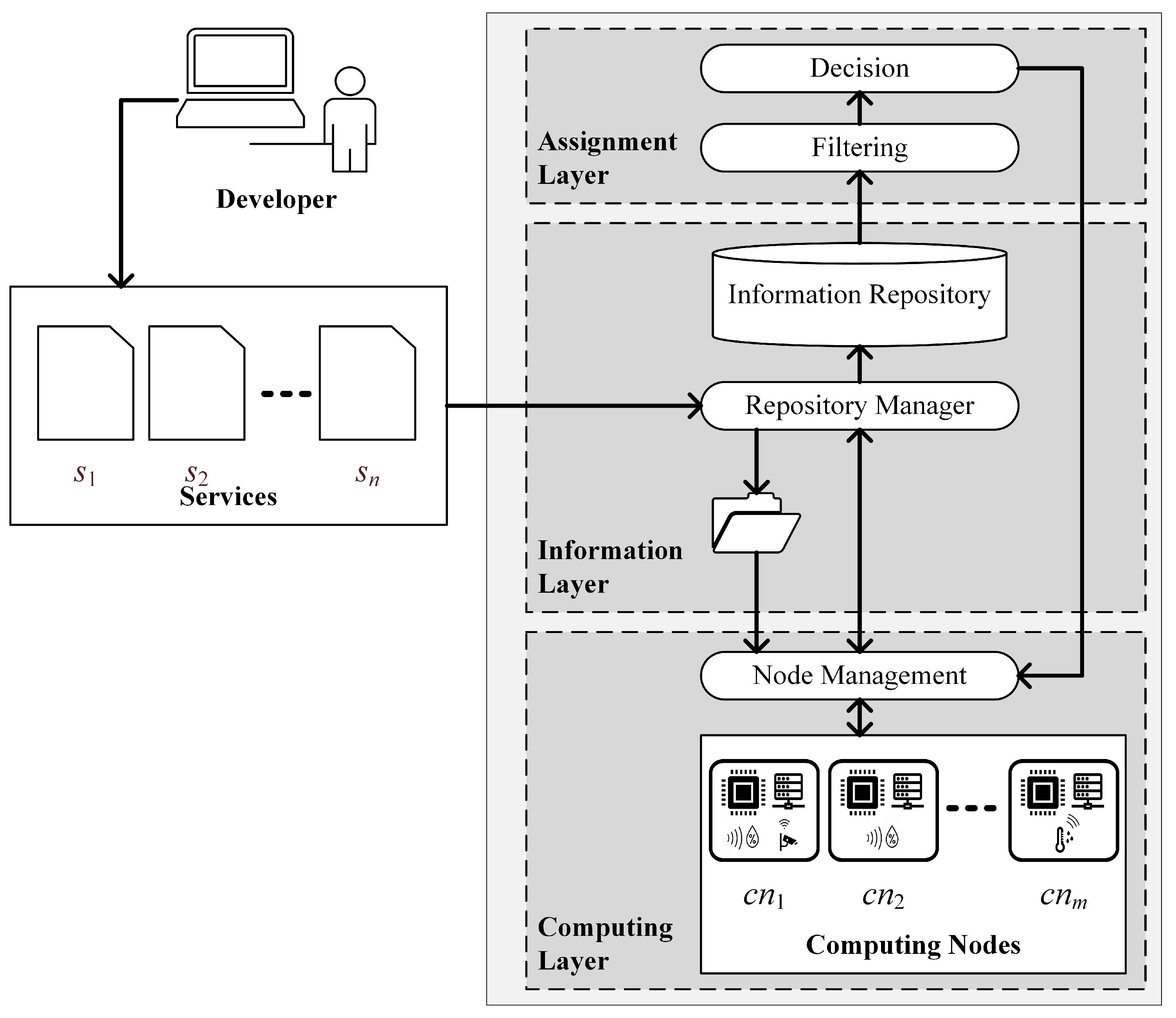
3. Proposed Framework

The architecture proposed in this work is shown in Figure 1. It tries to optimize the use of computational resources of IoT systems according to the needs of the software services that have to be computed. To do so, the solution executes an optimization process that first identifies the software and hardware needs, then identifies the available resources and finally performs the allocation of those resources to the software to be executed.

The proposed solution is composed of three layers: the computing layer, the information layer and the assignment layer. The computing layer consists of the computing nodes that will run software services and other functional resources such as sensors or cameras. The information layer contains data about the compute nodes in the system and their current available resources, as well as specifications of the services that need to be executed. Finally, the decision layer is in charge of processing all this information and planning the service assignments to the compute nodes.

In the following sections, we detail each of these layers.

3.1. Computing Layer

This layer is composed of hardware elements, which are mainly compute nodes and input/output devices (e.g., sensors, cameras, etc.). Computing nodes are an abstract representation for modeling computational devices of varying capacities. Examples of these nodes are Arduino-based development boards, Raspberry Pi, laptops, tablets, smartphones, servers, data centers, etc. Our work, in addition to taking into account the computational capacity, also considers functional resources offered by compute nodes. That is, a smartphone-based computing node is very likely to have a camera or some other type of sensor that the services can use. Or in the case of sensors connected to Arduinos or Raspberry Pi, the possibility of using other sensors connected to these devices opens the door to many possibilities. Our work also takes into account the physical location of each computing node.

The node management (NM) is in charge of managing the information of the compute nodes. The NM is responsible for collecting the information of each compute node and deploying the services on each of the nodes. The NM communicates with the repository manager (information layer) to update the list of available compute nodes and their resources state at a given time, in particular after deploying services on nodes. The NM receives, from the decision layer, the proposed allocation of services to computing nodes.

3.2. Information Layer

The information layer is in charge of managing all the existing information in the system. This layer contains information on the services and computing nodes with which the proposed system will work. This layer is composed of the information repository (IR) and the repository manager. The information repository is formed by a knowledge network that contains all the information related to the available computing nodes and the services that demand resources. The repository manager (RM) is in charge of registering the relevant information repository. The RM receives information about the compute nodes from the NM, and then the RM collects this information and inserts it into the knowledge network of the IR. The RM also receives the services to be executed by the compute nodes and a description of them. The RM processes the description of the services and inserts the information into the IR. The RM also stores those services in a repository connected to the NM, and then the NM will deploy, from that repository, the services on the corresponding compute nodes.

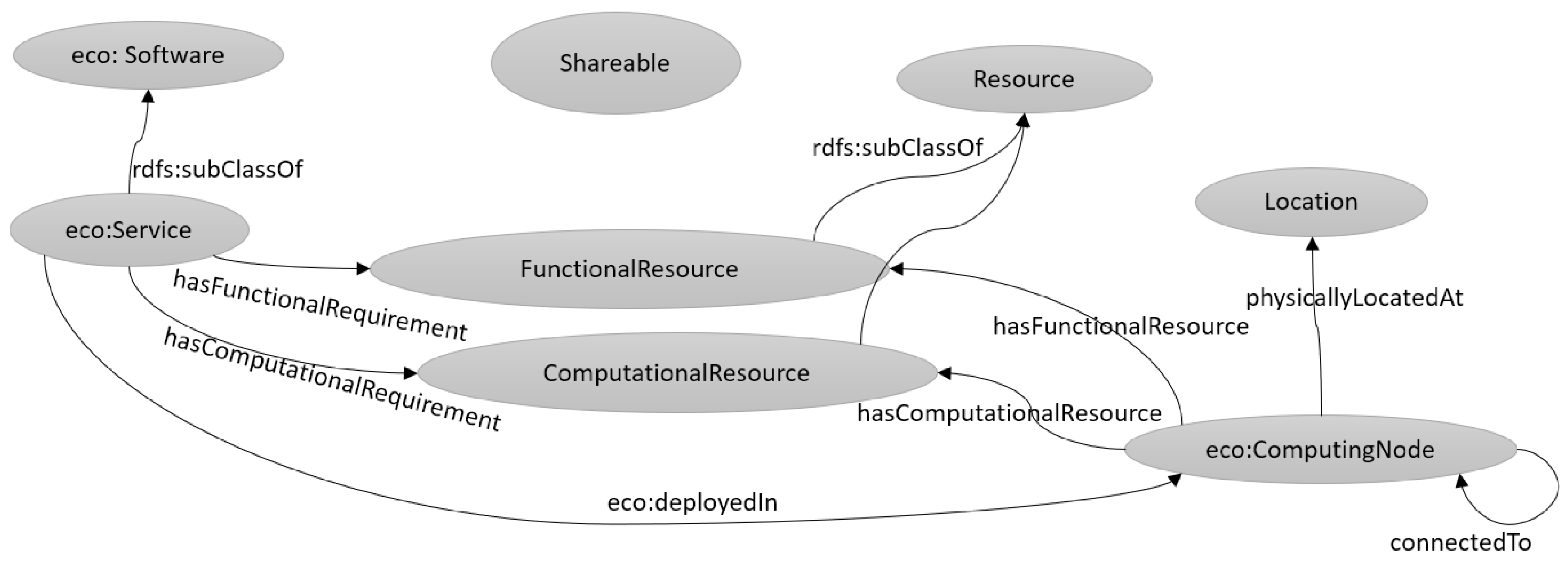
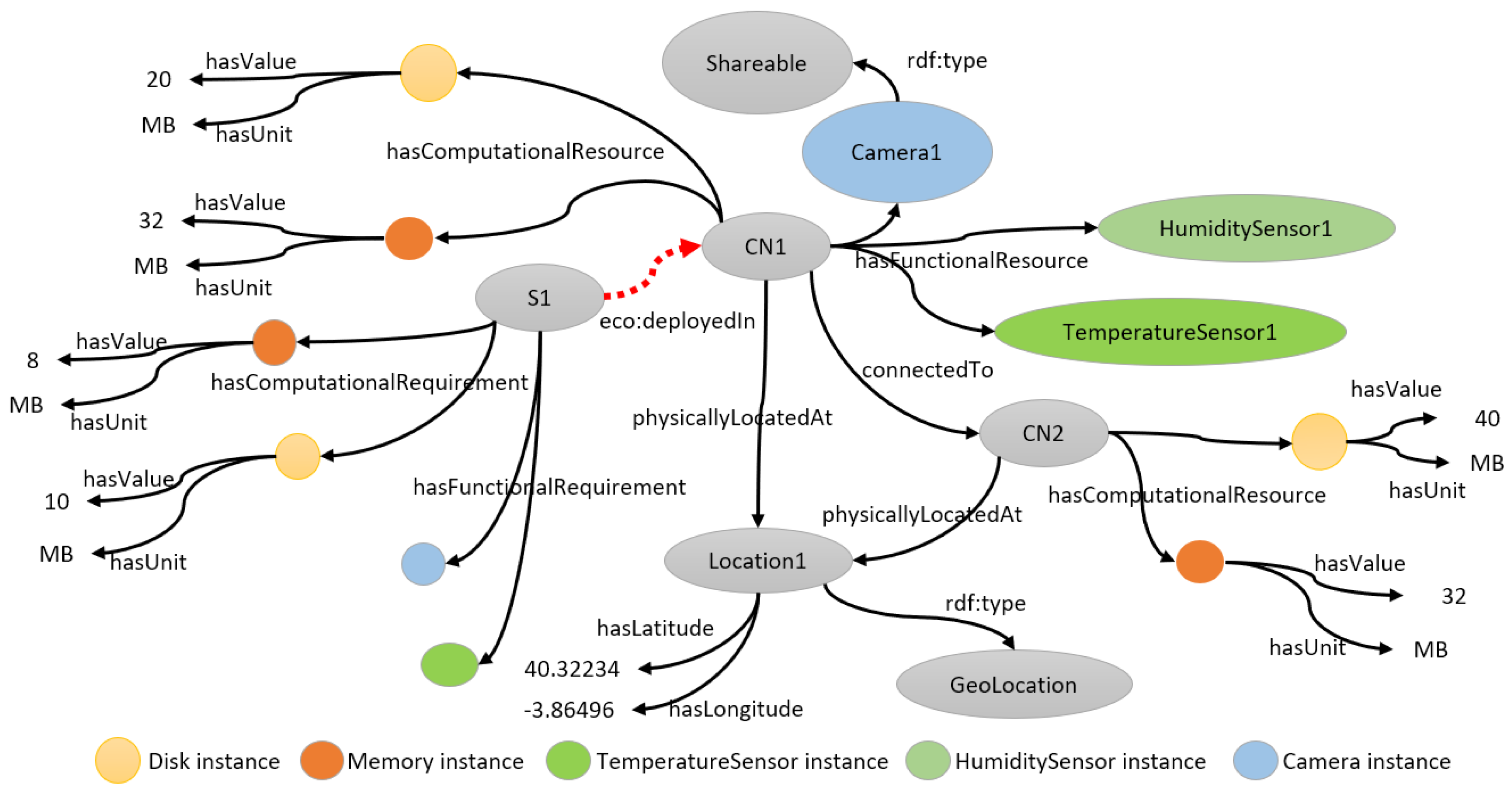
3.2.1. Knowledge Representation

For the management of the elements involved in such an ecosystem, we propose to use knowledge graphs [21], not only to model all the information available in the system but also to know how the information is related. The knowledge graph has a wide variety of key concepts in the domain of communications and computing. The knowledge graph proposed in this work is based on an extension of the OWL edge–cloud ontology (ECO) [27] developed in previous works. In this work, new elements have been added to the ECO to better represent and categorize the resources and requirements of the system. The ontology consists of several classes, data and object properties, which are semantically interconnected to accurately represent the relationships between concepts. The most relevant classes and properties are shown in Figure 2. In the following paragraphs, we describe the main elements of the ontology.

In our framework, there are two main types of entities: services and computing nodes. A service is the smallest software unit, and it can be of a certain type. For example, two meteorological stations may be running the same software to provide weather information. In this case, it is considered that they are two different services (of the same type), each of them running on different stations (devices). Depending on the purpose of the service and the functionality it provides, it can be deployed on IoT devices, on data centers hosted in the cloud or on fog devices.

Services can be run on hardware devices and machines. We denote those hardware elements as computing nodes. A computing node (CN) is hardware in which software can be installed and run. Computing nodes may have different computing resources, ranging from simple sensors and smart devices to powerful computers. Computing nodes have some available resources, which can be of two different types, namely computational (e.g., disk, RAM, CPU) and functional (e.g., camera, temperature sensor) resources.

This structure is represented in the ontology as a class called Resource and subclasses called ComputationalResource and FunctionalResource. Specific resources are represented as instances of such classes, and they are associated with each node with the properties hasComputationalResource and hasFunctionalResource, respectively.

Each service usually has a set of requirements. They refer to resources that services require for their functioning. Thus, we again distinguish between functional and computational requirements. Functional requirements are those necessary for a service to carry out its functions. For example, if the software requires special peripherals (e.g., a camera, temperature sensor, etc.), such software can only be installed in those computing nodes that provide those elements. Besides functional requirements, services may have some computational requirements such as the minimum RAM, disk space, CPU power, etc. In this case, instances of the same aforementioned (resource) subclasses are linked to services through the properties hasComputationalRequirement and hasFunctionalRequirement.

The physical location of resources plays an important role in our framework, especially for functional resources. For example, the location of a sensor can determine if it can be used for providing certain services. For this reason, we explicitly represent that information in our ontology using the class location and several subclasses that allow for the characterization of different types of locations (e.g., address, geolocation, etc.). This way, different types of locations can be expressed at different levels of granularity, like specific coordinates, regions or user-defined zones. The location of computing nodes and resources can be specified with the property physicallyLocatedAt. This property is defined as transitive (owl:TransitiveProperty), which means that it can be automatically inferred that, for example, a sensor is located at a university campus if it is located at a building in that campus.

Some functional resources may be shared among different computing nodes if they are located in the same physical location. For example, a service running on a computer could use a camera connected to another device in the same location (i.e., to take pictures from different fields). We assume each functional resource is connected to one computing node (i.e., only one node has a specific functional resource). In addition, such resources must be instances of the class shareable to distinguish which resources can be shared.

Table 1. Object Properties of the ontology, including the domain and range of each property. (Symm) and (Trans) indicate that the properties are symmetric and transitive, respectively.

ObjectProperty	Domain	Range
hasRequirement	Software	Resource
hasComputationalRequirement	Software	ComputationalResource
hasFunctionalRequirement	Software	FunctionalResource
hasResource	ComputingNode	Resource
hasComputationalResource	ComputingNode	ComputationalResource
hasFunctionalResource	ComputingNode	FucntionalResource
installedOn	Software	ComputingNode
connectedTo (Symm)	ComputingNode	ComputingNode
physicallyLocatedAt (Trans)	ComputingNode or Resource	Location

summarizes the object properties of the ontology.

In addition to these classes, the ontology provides a set of data properties to assign literal values to the entities. Some of them are described in

Table 2. Datatype properties of the ontology, including the domain and range of each property.

ObjectProperty	Domain	Range
hasLatitude	GeoLocation	xsd:double
hasLongitude	GeoLocation	xsd:double
hasUnit	ComputationalResource	xsd:string
hasValue	ComputationalResource	-

. The hasLatitude and hasLongitude properties are used to represent the latitude and longitude of a geographical location, allowing the assignment of numeric values that indicate the precise geographic location of an entity. The hasUnit property is used to specify the unit of measure associated with a numeric value, such as meters, kilograms or seconds. Finally, the hasValue property is used to assign numeric or other values to an entity in the ontology, representing quantitative information associated with that entity.

Note that when a computing node is running software, some resources are consumed (e.g., RAM). It is important to keep up-to-date information on the amount of available resources for each computing node. For this reason, it is expected that the value of this (hasValue) property changes dynamically.

Figure 3 shows an example of computing nodes and services represented through the entities defined in the ontology explained above. The main entities shown are service S1 and computation nodes CN1 and CN2. The model also indicates the requirements that S1 needs to function properly. These requirements are modeled through the hasComputationalRequirement property (two arcs) specifying that S1 requires 10 MB of memory and 20 MB of disk to work. This is represented by the entities of the types memory and disk, respectively, through the data properties hasValue and hasUnit discussed above. S1 has two functional requirements, represented through the hasFunctionalRequirement property: a camera and a temperature sensor.

The figure also shows the computational and functional resources of computing nodes CN1 and CN2. Using the hasComputationalResource property, the figure shows that CN1 has a disk capacity of 32 MB and 20 MB of memory. The property hasFunctionalResource is used to indicate that CN1 has a camera (Camera1), a humidity sensor and a temperature sensor.

Camera1 is shared by making it an instance of the shareable class. Thus, it is potentially accessible to CN2 since both CN1 and CN2 are connected (connectedTo relation) and they are physically located in the same place.

Note that, in this small example, S1 can be potentially deployed in CN1 (shown in Figure 3 as a dotted line) since S1’s requirements are fulfilled by CN1.

3.2.2. Inferencing and Querying the Model

Knowledge graph representations using formal ontologies (based on description logics) provide simple, easy-to-understand and flexible models to represent information. The model can be properly processed and automatic inferences can be carried out to obtain relevant information not initially made explicit.

The most common type of inference is probably the subsumption among classes (i.e., rdfs:subClassOf relations). Instances of a class can be implicitly derived from the analysis of the subclass-of relation in a taxonomy class structure.

Subproperty relations are less common but still very useful for inferring general relations from more specific ones. This is the case, for example, for resource or requirement types. Resources available at a node are those that are computational or functional resources (or any further subproperty relation, if any). All of them can be obtained since each of the three types of relations is defined as rdfs:subPropertyOf hasResource.

Moreover, more specific OWL characteristics can be exploited to endow the model with higher expressive power. In particular, we take advantage of the symmetric connectedTo property to represent logical networks of computing devices, without needing to make explicit the bi-directionality of computer connections. Finally, we defined the physicallyLocatedAt property as transitive, which means that we can derive the location of any element (e.g., a sensor) from the location of their container node.

The use of a knowledge graph to model the services and elements of a network over an information system is not only beneficial to know the connections and relationships between each of the elements of the infrastructure but also to model how some elements can influence the operation of others.

SPARQL queries can be used over the inferred model to extract relevant information. For example, Listing 1 shows a query that finds all computing nodes in which each service can be deployed according to their disk and memory computational requirements. A variation of that query can be easily generated on the fly to obtain all nodes with enough resources to deploy a specific service by first obtaining all required resources and then repeating the pattern in lines, e.g., 8–10 for each of them.

Listing 1: Example of query for obtaining pairs of services and computing nodes with enough availability of RAM and HDD for some computational requirements.

1    PREFIX owl : <http://www.w3.org/2002/07/owl#>

2    PREFIX rdf: <http://www.w3.org/1999/02/22-rdf-syntax-ns#>

3    PREFIX rdfs: <http://www.w3.org/2000/01/rdf-schema#>

4    PREFIX on: <https://www.ia.urjc.es/ontologies/networkOntology/>

5    SELECT DISTINCT ?serv ?cn

6    WHERE {

7                   ?serv rdf:type on:Service;

8                                 on:hasComputationalRequirement ?hddS;

9                                 on:hasComputationalRequirement ?memS.

10                   ?hddS rdf:type on:Disk;

11                                 on:hasValue ?valHDDS.

12                   ?memS rdf:type on:Memory;

13                                 on:hasValue ?valMemS.

14

15                   ?cn rdf:type on:ComputingNode;

16                               on:hasComputationalResource ?hddCN;

17                               on:hasComputationalResource ?memCN.

18                   ?hddCN rdf:type on:Disk;

19                                  on:hasValue ?valHDDCN.

20                   ?memCN rdf:type on:Memory;

21                                  on:hasValue ?valMemCN.

22

23                   FILTER(?valHDDS <= ?valHDDCN)

24                   FILTER(?valMemS <= ?valMemCN)

25  }

Another interesting query is shown in Listing 2. In this case, the query obtains all available resources (of any type) of each computing node. It includes them directly through both the computing node (line 5) and the shared resources owned by connected nodes located in the same area (lines 9–15).

Those queries are examples of the potential of using knowledge graphs with ontological schema. In Section 3.3, we present a method for assigning services to computing nodes based on clustering strategies.

We propose to take advantage of this idea to extract the relevant information before applying the clustering techniques presented in Section 3.3.2. In this paper, we optimize the allocation of software services to compute nodes depending on the characteristics of the nodes and the services. As described above, all this information is modeled in the knowledge graph, and it only needs to be extracted appropriately.

We used Protégé (https://protege.stanford.edu/, accessed on 20 January 2024)) for constructing the ontology. The Hermit OWL reasoner was used to check the consistency of the ontology. SPARQL queries and other automatic inferences were carried out using the Apache Jena (https://jena.apache.org/, accessed on 20 January 2024) framework.

Listing 2: SPARQL statement to obtain a list of nodes with available resources.

1    SELECT  DISTINCT ?computingNode ?res

2    WHERE {

3                      ?computingNode rdf:type on:ComputingNode.

4                      {

5                       ?computingNode on:hasResource ?res .

6                      }

7                      UNION

8                      {

9                        ?location rdf:type on:Location.

10                       ?computingNode on:physicallyLocatedAt ?location.

11                       ?computingNode on:connectedTo ?computingNode2.

12                       ?computingNode2 on:physicallyLocatedAt ?location.

13                       FILTER (?computingNode != ?computingNode2)

14                       ?computingNode2 on:hasResource ?res .

15                       ?res rdf:type on:Shareable.

16                      }

17    }

18    ORDER BY ?computingNode

3.2.3. Formal Representation

In this section, we present a more formal and compact version of the information provided by the information layer that is useful for the next stages of the assignment problem we address in this work.

Let S be the list of all services in the system,

$$S=[s_1,\dots ,s_i,\dots ,s_n]$$

(1)

where $s_i$ represents the specific service identified by i.

Let $CN$ be the list of all computing nodes,

$$CN=[c{n}_1,\dots ,c{n}_j,\dots ,c{n}_m]$$

(2)

where $c{n}_j$ represents a computation node.

The functional requirements for each service are in the list $FRS$ of all functional requirements:

$$FRS=[F{R}^{s_1},\dots ,F{R}^{s_i},\dots ,F{R}^{s_n}]$$

(3)

where $F{R}^{s_i}$ is a list that defines the functional requirements that service $s_i$ needs to operate. $F{R}^{s_i}$ is defined as follows:

$$F{R}^{s_i}=[locatio{n}^{s_i},f{r}_1^{s_i},\dots ,f{r}_k^{s_i},\dots ,f{r}_p^{s_i}]$$

(4)

where $locatio{n}^{s_i}$ represents a geolocated area of interest for service $s_i$ and $f{r}_k^{s_i}$, $k=1,2,\dots ,p$, are boolean values indicating whether or not each of the p functional requirements are needed by the service. The first element of the vector, $locatio{n}^{s_i}$, takes a value from a set of possible zones depending on the application domain. This parameter is usually important for services running on IoT devices (e.g., a temperature report on a specific field).

The list of computational requirements needed by services ($CRS$) is defined as follows:

$$CRS=[C{R}^{s_1},\dots ,C{R}^{s_i},\dots ,C{R}^{s_n}]$$

(5)

where $C{R}^{s_i}$ represents the computational requirements of service $s_i$:

$$C{R}^{s_i}=[c{r}_1^{s_i},\dots ,c{r}_l^{s_i},\dots ,c{r}_q^{s_i}]$$

(6)

where $c{r}_l^{s_i}$, with $l=1,2,\dots ,q$, are quantities that represent the value for a given l-th property (e.g., available RAM, available disk size, etc.).

Analogously to the definition of requirements for software services, we define functional and computational resources available in computing nodes as follows.

The list of functional resources provided by the computing nodes is as follows:

$$FRCN=[F{R}^{c{n}_1},\dots ,F{R}^{c{n}_j},\dots ,F{R}^{c{n}_m}]$$

(7)

where $F{R}^{c{n}_j}$ specifies the functional resources that computing node $c{n}_j$ provides. $F{R}^{c{n}_j}$ is defined as follows:

$$F{R}^{c{n}_j}=[locatio{n}^{c{n}_j},f{r}_1^{c{n}_j},\dots ,f{r}_k^{c{n}_j},\dots ,f{r}_p^{c{n}_j}]$$

(8)

Likewise, the computational resources provided by computing nodes are defined as follows:

$$CRCN=[C{R}^{c{n}_1},\dots ,C{R}^{c{n}_j},\dots ,C{R}^{c{n}_m}]$$

(9)

where $C{R}^{c{n}_j}$ specifies the computational resources that computing node $c{n}_j$ provides. $C{R}^{c{n}_j}$ is defined as follows:

$$C{R}^{c{n}_j}=[c{r}_1^{c{n}_j},\dots ,c{r}_l^{c{n}_j},\dots ,c{r}_q^{c{n}_j}]$$

(10)

3.3. Assignment Layer

The assignment layer is responsible for processing the information registered in the information repository (information layer) and calculates the allocation of services over the available compute nodes at a given time. It works in two stages. First, a filtering process is carried out in which compatible service–node pairs are matched (i.e., compute nodes with enough available resources to run services). Second, a decision process finds the best node–service allocation according to a given strategy.

3.3.1. Filtering

According to the framework in Figure 1, we need to obtain the possible allocations for each service, i.e., matching the resources required by every service with the adequate computing node. This matching process is made in two stages. First, we need to ensure that the functional requirements of service $s_i$ can be satisfied by the functional resources of the computing node $c{n}_j$. Formally,

$F{R}^{s_i}=[locatio{n}^{s_i},f{r}_1^{s_i},\dots ,f{r}_k^{s_i},\dots ,f{r}_p^{s_i}]$ is covered by

$F{R}^{c{n}_j}=[locatio{n}^{c{n}_j},f{r}_1^{c{n}_j},\dots ,f{r}_k^{c{n}_j},\dots ,f{r}_p^{c{n}_j}]$

if and only if $locatio{n}^{s_i}=locatio{n}^{c{n}_j}$ and $f{r}_k^{s_i}\to f{r}_k^{c{n}_j}$∀$1\le k\le p$, where $locatio{n}^{s_i}$ and $locatio{n}^{c{n}_j}$ are the place where $s_i$ requires the functional resource $f{r}_k^{s_i}$ and the place where $c{n}_j$ offers the functional resource $f{r}_k^{c{n}_j}$, respectively. Notice that $f{r}_k^{s_i}\to f{r}_k^{c{n}_j}$ specifies that all (boolean) functional requirements of service $s_i$ are covered by their corresponding functional resource of computing node $c{n}_j$ (i.e., if $f{r}_k^{s_i}=true$, then $f{r}_k^{c{n}_j}$ must be also true). This can be easily performed using SPARQL or any other piece of software.

Under these considerations, this first stage returns all scenarios of possible allocations for every service. For example, suppose that we have three services ($s_1$, $s_2$ and $s_3$) and four computing nodes ($c{n}_1$, $c{n}_2$, $c{n}_3$ and $c{n}_4$), which have the functional resources and locations shown in

Table 3. Functional and computational resources demanded by services ($s_i$) and offered by computing nodes ($c{n}_j$).

$FR=(location,camera,temperatureSensor,humiditySensor)$
$CR=(diskSpace,RAM)$
$s_i$	$F{R}^{s_i}$	$C{R}^{s_i}$	$c{n}_j$	$F{R}^{c{n}_j}$	$C{R}^{c{n}_j}$
$s_1$	$(zon{e}_1,true,true,false)$	$(10,8)$	$c{n}_1$	$(zon{e}_1,true,true,true)$	$(20,32)$
$s_2$	$(zon{e}_1,false,false,frue)$	$(10,24)$	$c{n}_2$	$(zon{e}_2,true,true,true)$	$(40,32)$
$s_3$	$(zon{e}_2,true,true,false)$	$(30,20)$	$c{n}_3$	$(zon{e}_1,true,false,true)$	$(30,32)$
			$c{n}_4$	$(zon{e}_1,true,true,true)$	$(20,16)$

.

According to the data of Table 3, $F{R}^{s_1}$ is covered by $F{R}^{c{n}_1}$ and $F{R}^{c{n}_4}$; $F{R}^{s_2}$ is covered by $F{R}^{c{n}_1}$, $F{R}^{c{n}_3}$ and $F{R}^{c{n}_4}$; and $F{R}^{s_3}$ is covered by $F{R}^{c{n}_2}$.

Taking into account only the functional aspect, the possible allocation scenarios are as follows: $s_1$ can be allocated in $c{n}_1$ or $c{n}_4$; $s_2$ can be allocated in $c{n}_1$ or $c{n}_3$ or $c{n}_4$; and $s_3$ can be allocated in $c{n}_2$. This result is graphically represented in Figure 4.

The second stage implies considering the computational requirements of each service and the computational resources of every computing node. In this case, we need to ensure that the computational demand of service $s_i$ can be covered by the computational resources of computing node $c{n}_j$. Formally,

$C{R}^{s_i}:[c{r}_1^{s_i},\dots ,c{r}_l^{s_i},\dots ,c{r}_q^{s_i}]$ is covered by $C{R}^{c{n}_j}:[c{r}_1^{c{n}_j},\dots ,c{r}_l^{c{n}_j},\dots ,c{r}_q^{c{n}_j}]$

if and only if $c{r}_l^{s_i}\le c{r}_l^{c{n}_j}$∀$1\le l\le q$.

The example in Table 3 also includes two computational resources: disk space and RAM (both expressed in GB). Consequently, $C{R}^{s_1}$ is covered by $C{R}^{c{n}_1}$, $C{R}^{c{n}_2}$, $C{R}^{c{n}_3}$ and $C{R}^{c{n}_4}$; $C{R}^{s_2}$ is covered by $C{R}^{c{n}_1}$, $C{R}^{c{n}_2}$ and $C{R}^{c{n}_3}$; and $C{R}^{s_3}$ is covered by $C{R}^{c{n}_2}$ and $C{R}^{c{n}_3}$

Therefore, taking into account the computational aspects, the possible allocation scenarios are as follows: $s_1$ can be allocated in $c{n}_1$, $c{n}_2$, $c{n}_3$ or $c{n}_4$; $s_2$ can be allocated in $c{n}_1$, $c{n}_2$ or $c{n}_3$; and $s_3$ can be allocated in $c{n}_2$ or $c{n}_3$. Computational nodes and services can be represented in an n-dimensional space according to their available and required resources, respectively. Figure 5 shows the 2D representation of our example. Each node $c{n}_i$ defines an area (colored differently, although there are some overlapping) in such a way that services inside can be deployed in it. A different picture is presented for each service, where black nodes allow for possible deployments in them, while white nodes do not have enough resources.

Finally, unified scenarios from both functional and computational perspectives are as follows: $s_1$ can be allocated in $c{n}_1$ or $c{n}_4$; $s_2$ can be allocated in $c{n}_1$ or $c{n}_3$; and $s_3$ can be allocated in $c{n}_2$ (Figure 6).

The filtering process can be easily implemented with different programming approaches. In particular, SPARQL queries can be easily created to carry out the filtering task. We already presented in Listing 1 an example of filtering computing nodes that are adequate for each service according to some computational requirements. For a specific case, like the one shown in Table 3, the corresponding query can be created on the fly to account for all the requirements (FR and CR) considered in the system.

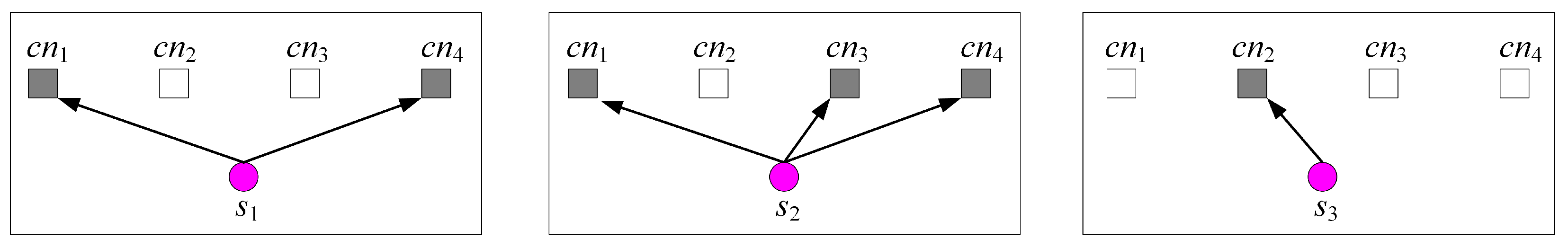
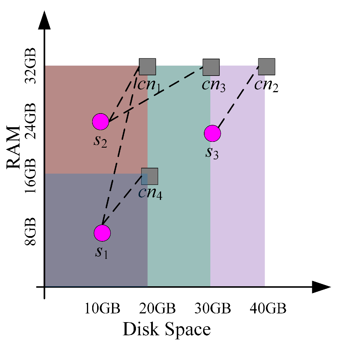
3.3.2. Decision

Once the integrated filtering scenario has been obtained, we need to analyze the computing resources adjustment to obtain an adequate allocation. This aspect is very important because the quantity of requirements is bigger than the quantity of available resources, and, consequently, bad allocation decisions could waste these resources.

Evidently, after the filtering process, there can be a large number of possible assignment combinations and it can exponentially grow when more services and computing nodes are added to the IoT infrastructure. Additionally, this type of environment is very dynamic, and some resources are released when a service has finished its task, which requires revising the allocations. Likewise, new services may appear on the fly and need nodes in which to be deployed.

After the filtering process, each computing node has a list of services that it can host considering both functional and computational aspects. The Possible Allocation Service $PAS$ list contains one list, $pa{s}^{c{n}_j}$, for each computing node, $c{n}_j$, with all services $s_i$ that it could allocate. Formally,

$PAS=[pa{s}^{c{n}_1},\dots ,pa{s}^{c{n}_j},\dots ,pa{s}^{c{n}_m}]$ where $pa{s}^{c{n}_j}$ is a list of services $s_i$ assignable to $c{n}_j$ with $1\le i\le n$.

For example, under these considerations, the $PAS$ list for the integrated filtering scenario of Figure 6 is as follows:

$PAS=[pa{s}^{c{n}_1},pa{s}^{c{n}_2},pa{s}^{c{n}_3},pa{s}^{c{n}_4}]$ with $pa{s}^{c{n}_1}=[s_1,s_2]$, $pa{s}^{c{n}_2}=\left[s_3\right]$, $pa{s}^{c{n}_3}=\left[s_2\right]$, $pa{s}^{c{n}_4}=\left[s_1\right]$.

Because a computing node can execute multiple services at the same time and it is possible to allocate a service on any of several computing nodes, there is no single combination of allocations. Here, we introduce a key concept, the distances between computing nodes and services. These distances indicate the difference between computational resources demanded by service $s_i$ and the computational resources offered by computing node $c{n}_j$. In this way, it is possible to compute the distances between every computing node and each service in its list. A distance equal to zero indicates a perfect match between the computational resources demanded by $s_i$ and the computational resources offered by $c{n}_j$, which means that all resources at $c{n}_j$ are dedicated to $s_i$. Evidently, with potentially many possible combinations of allocations, the situation of a perfect match is not the usual, and finding a good configuration is a complex task.

To deal with this situation, we follow a clustering approach, in which the objective is to create m clusters of services (one per computing node), each cluster containing the services that will be allocated in each node. For each integrated filtering scenario, we propose to use a variation of agglomerative hierarchical clustering (AHC) [5,6] based on computational resource matching. In this case, when the best match is found and the service is allocated, the resources of the corresponding computing node are decremented and the distances between the rest of the services and the computing node are recomputed. This variant of the AHC (that is, the recalculation of distances after assignment) is necessary since the allocation of a service to a computing node decreases the available resources of the node.

As we said before, the distance between $c{n}_j$ and $s_i$ ($d(c{n}_j,s_i)$) is a measure that indicates how adequate computing node $c{n}_j$ is to host service $s_i$. Depending on the context, $d(c{n}_j,s_i)$ can be the Euclidean distance or any other similarity measure that considers the magnitude of each computational resource. This measure is necessary to generate clusters according to some clustering strategy to select the allocation order. Note that, due to the dynamics of the allocation, the order of allocation is very important. For example, if the priority is to assign services to the computing nodes that best fit their needs, each node will probably only allocate one service. This implies that, after the assignment, the computing nodes that have the greatest capacity might remain without assignments. On the contrary, if the nodes with the highest capacity are assigned first with services that require few resources, the services with higher requirements may be not allocated because the only computing nodes available do not have sufficient resources.

In this work, we propose four clustering strategies for assigning a service $s_i$ to a computing node $c{n}_j$:

(a)

$minMin$. The minimum of the shortest distance of each $pa{s}^{c{n}_j}$. This strategy selects the pair ($s_i$, $c{n}_j$) from $pa{s}^{c{n}_j}$ where the amounts of resources required by the service and offered by the computing node are as similar as possible.

(b)

$maxMin$. The maximum of the shortest distance of each $pa{s}^{c{n}_j}$. This strategy selects the pair ($s_i$, $c{n}_j$) from $pa{s}^{c{n}_j}$ where the amounts of resources required and offered are similar. That is, it selects the $c{n}_j$ whose minimum distance to services is the highest among the computing nodes. It can be seen as a relaxation of minMin, where it still prefers small distances but by selecting the maximum of the distance it leaves the rest of the resources of $c{n}_j$ available for another possible allocation.

(c)

$minMax$. The minimum of the greatest distance of each $pa{s}^{c{n}_j}$. This strategy selects the pair ($s_i$, $c{n}_j$) from $pa{s}^{c{n}_j}$ where the amounts of resources required and offered are quite different. This strategy promotes the allocation of services that require few resources in computing nodes with a low availability of such resources.

(d)

$maxMax$. The maximum of the greatest distance of each $pa{s}^{c{n}_j}$. This strategy selects the pair ($s_i$, $c{n}_j$) from $pa{s}^{c{n}_j}$ where the amounts of resources required and offered are very different. This strategy promotes the allocation of services that require few resources in computing nodes with a high availability of said resources.

Although the $minMin$ and $maxMin$ strategies are similar to the $single$-$link$ and $complete$-$link$ strategies, respectively [5,6], they are slightly different because when a service is assigned to a computing node the service is not taken into account for the next distance calculations. Because the resources of the selected computing node decrease, the distances between all remaining services and the node must be recalculated.

The allocation process is made until all services $s_i$ are allocated or there are no more computing nodes $c{n}_j$ with an available capacity to allocate another service. Finally, the list of services allocated in each computing node is stored in the allocated services ($ASs$) list. This set contains a list $a{s}^{c{n}_j}$, for each computing node $c{n}_j$, with all services $s_i$ allocated in it. The whole process is shown in Algorithm 1.

Algorithm 1: Clustering-based allocation

Algorithm 1 receives the Possible Allocation Service ($PAS$) list, the Computational Resources lists for each service and each computing node ($CRS$ and $CRCN$, respectively), the clustering strategy ($clustStrategy$) and the distance function ($distFunction$) to use. Note that although the $PAS$ list is obtained after the filtering process, it is necessary to know specifically what the requirements of the services and the capabilities of the computing nodes are; these data are contained in the $CRS$ and $CRCN$. Additionally, it is also necessary to know what clustering strategy will be used and how the distance between the service requirements and the resources available in the computing nodes will be measured. These last two characteristics provide great flexibility to the proposed model since any clustering strategy can be used with any distance measure according to the problem domain. As output, Algorithm 1 returns Allocated Services $ASs$ list.

At the beginning (lines 2–4), each $ASs$ list is initialized with the empty list to add every service $s_i$ to the corresponding best computing node $c{n}_j$ according to the specified clustering strategy. The main process is made in the loop between lines 5 and 15.

The loop repeats while there are possible unresolved allocations (line 5), i.e., if there is any non-empty list in the $PAS$ list. If that is the case, using the $PAS$, $CRS$ and $CRNC$ lists and the $distFunction$, the list of distances ($DS$) between all services of every list $pa{s}^{c{n}_j}$ and the corresponding $c{n}_j$ is calculated using the $computeDist\left(\right)$ function (line 6). In this way, for every list $pa{s}^{c{n}_j}$ in the $PAS$ list, there is a corresponding list $d{s}^{c{n}_j}$ in the $DS$.

When all distances are computed, the $findBestMatch\left(\right)$ function is used to obtain the effective service allocation (line 7). This function returns the pair ($s_{best}$, $c{n}_{best}$) that corresponds to the best allocation available according to the selected clustering strategy.

After that, service $s_{best}$ is added to the Allocation Service list of node $c{n}_{best}$, i.e, $a{s}^{c{n}_{best}}$. Notice that each list $a{s}^{c{n}_j}$ is built incrementally. If it is not possible to allocate any service to any $c{n}_j$, as its list will be empty after completing the process, i.e., $a{s}^{c{n}_j}=\left[\right]$.

Then, with the best allocation found, the required computational resources of the $s_{best}$ are discounted from the offered computational resources of the $c{n}_{best}$ (lines 9–11). Notice that this discount in the computing node is made for every type of resource.

Afterwards, the $removeService\left(\right)$ function removes $s_{best}$ from all $PAS$ lists that contain it, and the process is repeated until there are no services that can be allocated to the computing nodes (lines 12–14). Finally, the allocated services ($AS$) list is returned in line 16.

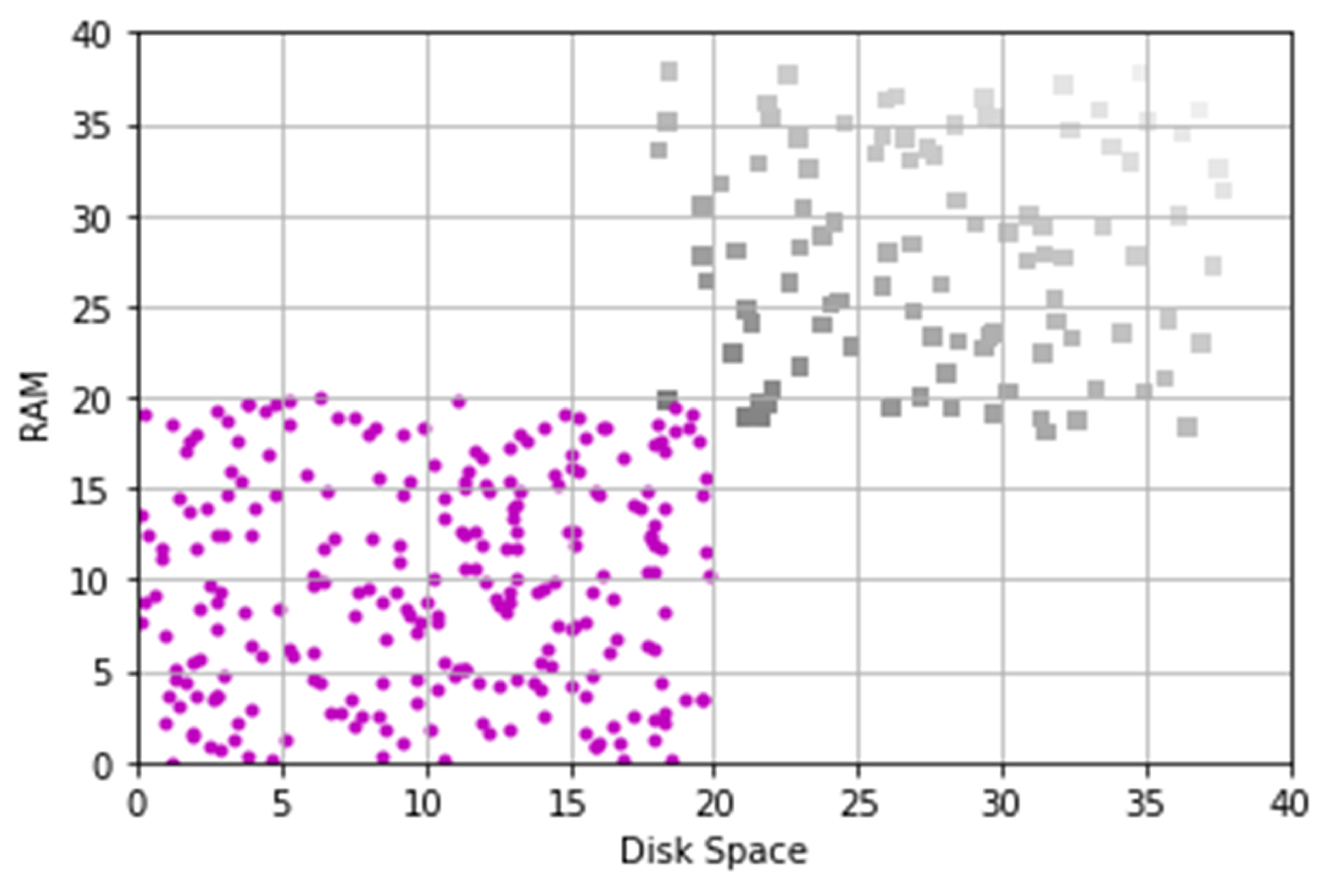
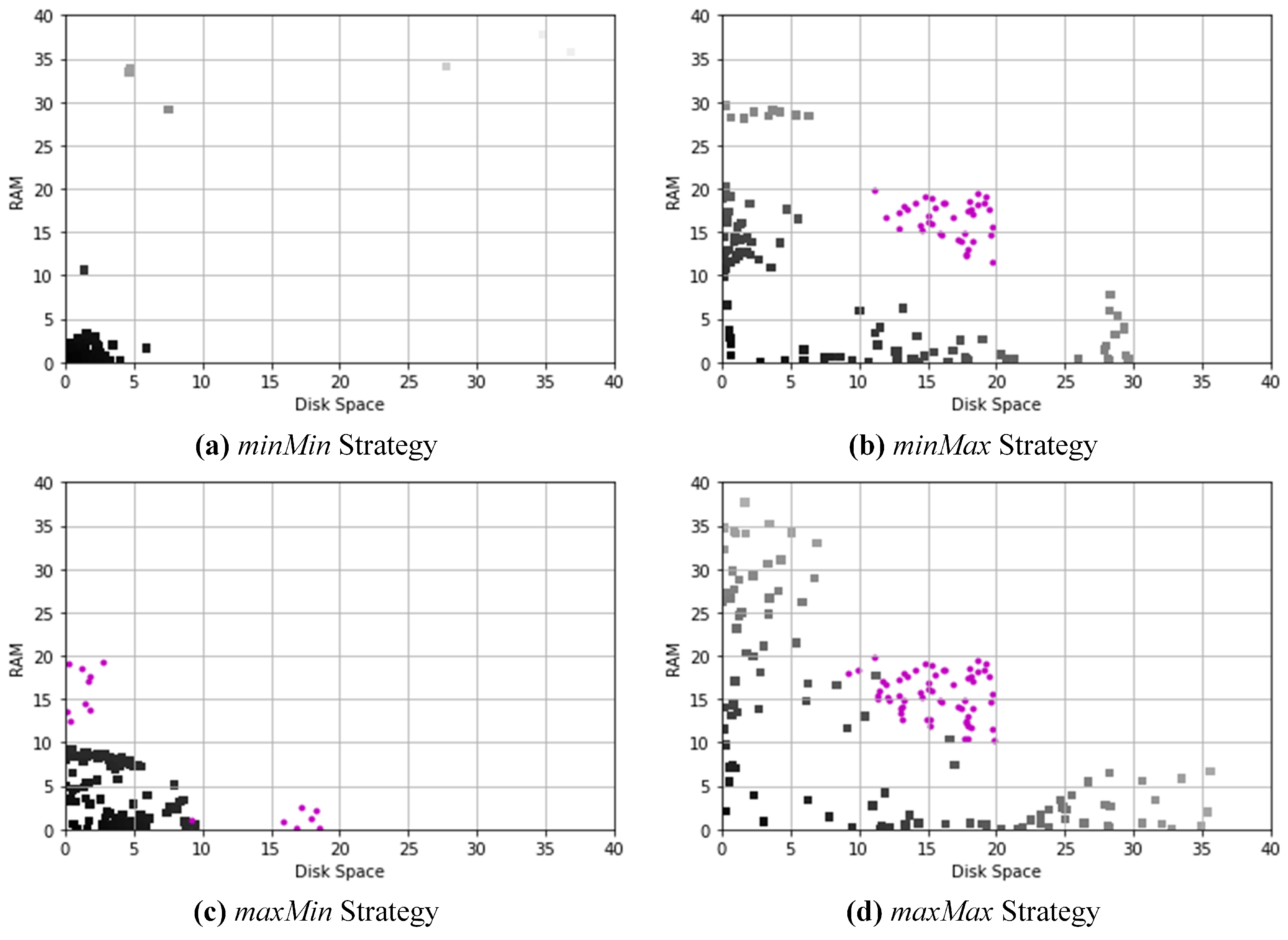
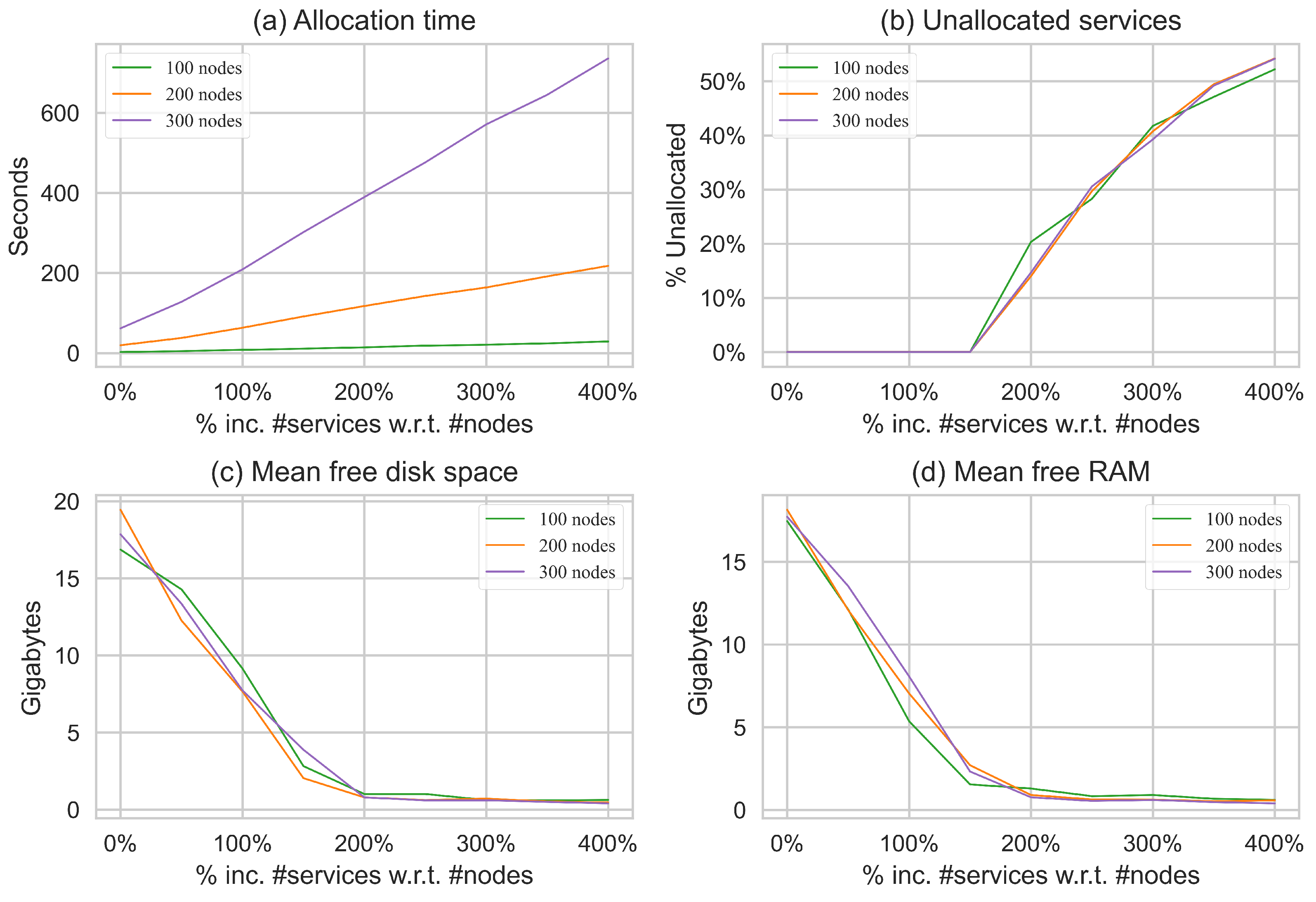
4. Allocation Experiments

In Section 3, we used a small illustrative running example to explain the different aspects of our service allocation framework. In this section, we focus on evaluating the four strategies proposed in Section 3.3.2.

Once the integrated scenario is obtained, that is, after the filtering stage, the effective allocation of the services to the computing nodes must be carried out. To do that, only the computational resources demanded by the services and offered by the computing nodes should be considered. In this example, 250 services and 100 computing nodes were generated. Two computational resources were considered: disk space and RAM. The integrated scenario is shown in Figure 7.

The disk space and RAM demanded by services, represented by magenta circles in Figure 7, were uniformly generated in the range $[0, 20]$ GB. Similarly, the disk space and RAM offered by the computing nodes, represented by gray squares in Figure 7, were uniformly generated in the range $[18, 38]$ GB. The selection of these parameters was based on the fact that the number of services is more than twice the number of computing nodes and each node could host two services on average. Additionally, the distribution of the magnitudes of disk space and RAM allows for a high number of combinations of possible allocations. This aspect is very important to test the clustering strategies.

To make the allocation process efficient, it is necessary to consider simultaneously the two dimensions, disk space and RAM. In this way, the Euclidean distance was selected to determine the adjustment degree between the demand and offer of resources.

Under these considerations, the four clustering strategies described in Section 3.3.2 were tested. Specifically, using Algorithm 1, the $minMin$, $maxMin$, $minMax$ and $maxMax$ strategies were used to allocate the services of the integrated scenario. The results are shown in Figure 8.

Note that in Figure 7 and Figure 8 the computing nodes were identified using a grayscale according to the availability of their resources, that is to say, dark gray for computing nodes with few available resources and light gray for those with many available resources.

Simulations show that the best allocation results are obtained (i.e., more services are allocated) when using the $minMin$ and $maxMin$ strategies (Figure 8a,c). The $minMin$ strategy (Figure 8a) has allocated all services, while only a few services have not been allocated using the $maxMin$ strategy (Figure 8c). This aspect is very important because when the allocation is complete, the response time of the entire allocation system decreases. Another interesting aspect is that, at the end of the allocation process, most of the nodes have few resources available, i.e., below 10 GB for both disk space and available RAM. This has two important considerations: on the one hand, there is an adequate use of the available resources, but, on the other hand, there could be an overload on the computing nodes. This second consideration indicates a drawback since if one of those overloaded computing nodes goes offline there will be no availability in other nodes to reallocate the services running on it.

Regarding the $minMax$ and $maxMax$ strategies, the final allocations are quite different (Figure 8b,d). First of all, more than ten percent of services are not allocated to any computing node. This is a drawback since, as seen previously for the $minMin$ strategy, there is a solution to this allocation problem in which all services are allocated to a node. Consequently, since all those services mentioned have not been allocated, the response time for these services will increase considerably, reducing the performance of the entire allocation system. Furthermore, it can be observed that non-allocated services are those that have a greater demand for computational resources. This shows that these strategies do not adequately manage the use of resources. Contrary to what was observed with the $minMin$ and $minMax$ strategies, there is not a great overload in all computing nodes, but there is a great consumption of one of the two resources available in each node. Indeed, if the available resources of several nodes of final allocation could be combined, all services not allocated would be covered. This aspect is another drawback because if any computing node goes offline, it is unlikely that another node that does not have enough resources can be used to reallocate the services of the computing node that went offline.

The simulations indicate that the minMin strategy provides the best results for service allocation. Although the simulations were configured with a fixed number of compute nodes and services, it is also necessary to test the scalability of the model. This involves analyzing the behavior of the model by varying the number of compute nodes and services. To achieve this, we propose simulating assignments with 100, 200 and 300 computing nodes while increasing the number of services from 0% (i.e., the same number of computing nodes) to 400% more services than computing nodes (with increments of 50% for each scenario). All simulations were conducted using Python 3.11.5 64-bit on an AMD Ryzen™ 5 4500U with a Radeon™ Graphics 2.38 GHz processor and 8 GB of RAM. The results are presented in Figure 9.

In Figure 9a, the allocation time for each number of compute nodes is shown as the number of services increases. It can be observed that the computation time grows linearly instead of exponentially, which is what one would expect. This is because after a 150% increase some services cannot be allocated to any compute node and are removed from the comparison process. As a result, the computation time is reduced significantly, and the increase becomes linear. However, if we compare the time difference between the curves for each number of nodes, we can see that the time increase is exponential. This is because the number of initial comparisons for each number of compute nodes varies exponentially. For example, initially, for 100 nodes there are 10,000 comparisons; for 200 nodes there are 40,000 comparisons; and for 300 nodes there are 90,000 comparisons. When we add the increase in the number of services per simulation to this, the difference in allocation times becomes significant.

In terms of the allocation time, it is observed that the performance drops considerably for numbers of compute nodes above 100. This issue can be resolved by using more powerful processors or applying distributed processing strategies. However, it is also recommended to analyze and improve the allocation algorithms.

When considering the number of unallocated services, the minMin strategy works effectively. For the simulations, it was assumed that a computing node could contain, on average, more than two services, i.e., the number of services is 100% greater than the number of computing nodes. The minMin strategy allocates services by searching for the best possible combination at each point in time, as illustrated in Figure 9b. It can allocate services up to 150% more than the number of nodes. However, beyond that point, the number of unallocated services increases exponentially.

The graphs depicting RAM and disk resource allocations in Figure 9c,d show a similar pattern to the previous description. When the number of services increases by over 150% with regards to the compute nodes, the available resources drop to such a low level that no further allocations are possible. This level remains constant no matter how much the number of services is increased. As mentioned in the first simulation, the minMin allocation strategy leads to an overload on the compute nodes. This is a significant factor since the failure of any one compute node would release several services that could not be re-allocated on other nodes.

To summarize, under the established conditions, the proposed model performs well for scalability conditions in terms of the number of services that each computing node can physically allocate.

5. Discussion

In this section, we include a discussion on several issues that remain open for further investigation, in which we provide some initial ideas for further development. In addition, we put our service allocation proposal in the context of other approaches.

5.1. Dynamic Adaptation of the Allocation Process

The distribution of services is a task that constantly changes, affecting the allocation process. Changes in the environment can modify the allocation conditions, and appropriate mechanisms are needed to maintain the system’s efficiency. The system itself is dynamic, and changes to the execution or termination of a service, as well as modifications to functional or computational requirements, can alter the environment. Some situations can cause unforeseen disturbances, such as one or more compute nodes starting up or turning offline. All of these alterations in the environment require adaptation mechanisms to ensure the system functions correctly.

This paper proposes a model that is capable of handling various situations by utilizing a repository manager to constantly monitor services and a node manager to supervise computing nodes. The model can detect changes and make the appropriate modifications to allocations. In this way, there are two types of tasks involved: monitoring and prediction.

Monitoring involves ensuring that the services are operating correctly on the nodes and, if there are any changes, whether due to normal system operations or not, making the necessary adjustments in the allocation. For instance, if a new service is requested, one of the proposed strategies can be used to determine the most suitable computing node. When a service is terminated and resources are released, it should be determined whether it is necessary to transfer the service to another node that is less overloaded due to the release of resources. Additionally, in the event of possible failures of computing nodes, the allocation algorithm should be executed for services that have been left without a node to run.

The task of prediction involves determining whether the allocation strategy needs to be changed to avoid node overload. This means that based on the current resource occupancy values and service arrivals (quantity and resources demanded), the node and repository managers must decide whether to modify the current allocations or not to increase the overall system efficiency. It is important to note that this prediction task should be performed alongside the monitoring task, as the primary objective is to ensure the efficiency of the current operation.

5.2. Relation to Other Allocation Approaches

There are multiple mechanisms for the allocation of tasks on nodes, from traditional approaches based on First-Come-First-Served (FCFS), Shortest Job First (SJF), Round Robin (RR), Min-Min and Max-Min algorithms [28,29,30], and even to more complex approaches based on machine learning (ML)- based intelligent approaches [31]. These works present solutions to manage task allocation using virtualization technologies, for example, virtual machines (VMs), in a cloud environment. These solutions assign tasks to the most appropriate compute nodes that are configured, in the form of a virtual machine (VM), in a cloud computing environment. Working in a cloud ecosystem facilitates the assignment process between task and compute node because the compute nodes are very similar and are geographically located in the same place. Works such as [32,33,34] present mechanisms for task allocation over distributed nodes between fog and cloud environments. Taneja and Davy [32] introduce an approach based on directed acyclic graphs where nodes have three attributes, the CPU, RAM and bandwidth, and also proposes an algorithm to match each task with its most suitable available node considering cloud and fog hosted nodes. In [33], dynamic service placement is proposed to minimize the transmission time, computational delay and migration delay when transferring the task to the corresponding node. In [34], a Petri net-based strategy is proposed to predict the time and price required to complete a task taking into account the reliability of the fog computing resources.

In general, these approaches do not take into account the heterogeneity of nodes and tasks, which is important to consider. Other works such as [35,36] take into account the heterogeneity of nodes and tasks and try to balance the load by minimizing the specific resources to assign tasks to each node. In [35], a multi-objective algorithm was used to optimize the time delay and energy consumption in a fog and cloud architecture. Xu et al. [36] present an algorithm for load balancing and resource allocation among different nodes based on their computational capacity, memory storage and bandwidth. Tasks are ranked based on the requested compute nodes and the predefined start time. A similar approach is explored in [37]. These approaches usually assume that all services are requested at the same time, which makes their models unable to cope with dynamic changes in traffic and different workload rates.

In this work, we propose a solution to work in environments composed of heterogeneous nodes (formed by devices) that can also be geographically distributed. That is, the available nodes are not located in the same data center, and each node can have unique characteristics. In addition, we consider not only computational resources but also functional resources and the possibility of sharing functional resources among multiple nodes in order to satisfy the task needs.

5.3. Quantifying Distances between Computational Resources

The proposed clustering approach to allocate services to compute nodes requires some notion of distance between nodes and services. Designing distance functions is natural if nodes/services can be characterized in terms of a set of numerical attributes. This is the case of the examples used in this paper, where RAM and disk space attributes are used to define service computational requirements and available resources. In addition, these numbers are further used to update (reduce) the newly available resources of a node if a service is assigned to it. However, not all resources are easy to express with numbers. This is the case, for example, of CPU processing power. It is not easy to represent with numbers the processing capability of CPUs, the processing need of a service, how much processing availability is reduced if a service is running in a CPU, etc. How to deal with these types of attributes requires further research. One idea to address this is to describe a catalogue of CPU types (maybe plus some configurations), which could be ordered by their computing power. For example, the following could represent a preference order ($x\succ y$, x is preferred over y) among CPUs:

Apple M2 Ultra≻Apple M1 Ultra $\succ \cdots \succ$Raspberry Pi 5≻Raspberry Pi Zero≻Arduino Mega 2560.

With such a definition, and assuming it is possible to identify which minimum CPU type is required by a service, it could be possible to at least filter out the nodes that do not comply with the minimum requirements. Calculating distances between CPU types is even more complex. A simple way could be to use the distance in the preference-ordered list of CPU types. However, that would assume a homogeneous distribution of different “CPU power” values in the list.

6. Conclusions and Future Work

In this paper, a service allocation framework based on hierarchical clustering was proposed and described. The proposed framework is divided into three layers. First, the computing layer includes the hardware components (computing nodes) in which software services are executed. Second, the information layer provides specifications of software services’ requirements and computing nodes’ available resources. We presented an ontology-based knowledge graph approach, which provides inference potential and flexibility for model extension. Third, the assignment layer is in charge of deciding the best allocation of services to nodes. This process is carried out in two stages: filtering and assignment. The filter component contributes to reducing the number of allocation combinations by analyzing functional and computational restrictions. Finally, the decision component builds an integrated allocation scenario for all services and computing nodes and calculates the assignment using hierarchical clustering. Four clustering strategies have been suggested to decide the service allocation order, prioritizing the assignment of certain nodes (e.g., with more capacity), establishing balancing conditions or preserving certain resources.

Experimental simulations were performed to test four clustering strategies using an integrated scenario with a high demand for resources. Results show that the $minMin$ and $maxMin$ strategies show similar behavior, allocating the services appropriately. Although the $minMin$ strategy has been the only one to allocate all services, the $maxMin$ strategy has not been able to find the perfect allocation for a few nodes. According to the results, both strategies efficiently fit the resource requirements of the services to the availability of resources in the computing nodes. However, this efficiency in allocation reduces the execution time of services but produces a large overload on most computing nodes.

The results obtained also show that the $minMax$ and $maxMax$ strategies have some similarities in their behavior. However, unlike the $minMin$ and $maxMin$ strategies, it can be observed that more than ten percent of services are not allocated at the end of the simulation. This drawback affects the overall response time of the services. Furthermore, an overload of most of the computing nodes is observed, but unlike what happens with the $minMin$ and $maxMin$ strategies, this overload is only on one of the two types of resources defined for the simulations. This indicates poor efficiency in managing the available resources of the computing nodes.

Finally, simulations show that it is possible to face the service allocation problem with the proposed framework using the proper combination of the distance function with the clustering strategy. In addition, the proposed framework is flexible and allows the use of any distance measure and any clustering strategy, beyond those presented in this article.

There are several lines of research that we are focusing on. First, we are working on richer semantic models to specify functional requirements/resources. Additionally, we are working on testing different distance and similarity functions to use non-numeric values for the clustering. Also, we are working on reconfiguration strategies to face dynamic conditions, such as service arrivals, the releasing of resources and node reconfigurations. In this sense, we are working on simulations extended over time, incorporating dynamic events of both time-varying services and possible computing node crashes.

References

- Yousefpour, A.; Fung, C.; Nguyen, T.; Kadiyala, K.; Jalali, F.; Niakanlahiji, A.; Kong, J.; Jue, J.P. All one needs to know about fog computing and related edge computing paradigms: A complete survey. J. Syst. Archit. 2019, 98, 289–330. [Google Scholar] [CrossRef]
- Ullah, A.; Dagdeviren, H.; Ariyattu, R.C.; DesLauriers, J.; Kiss, T.; Bowden, J. Micado-edge: Towards an application-level orchestrator for the cloud-to-edge computing continuum. J. Grid Comput. 2021, 19, 47. [Google Scholar] [CrossRef]
- Kimovski, D.; Matha, R.; Hammer, J.; Mehran, N.; Hellwagner, H.; Prodan, R. Cloud, Fog, or Edge: Where to Compute? IEEE Internet Comput. 2021, 25, 30–36. [Google Scholar] [CrossRef]
- Karanik, M.; Bernabé-Sánchez, I.; Fernández, A. Edge Service Allocation Based on Clustering Techniques. In Proceedings of the Trends in Sustainable Smart Cities and Territories; Castillo Ossa, L.F., Isaza, G., Cardona, Ó., Castrillón, O.D., Corchado Rodriguez, J.M., De la Prieta Pintado, F., Eds.; Springer: Cham, Switzerland, 2023; pp. 429–441. [Google Scholar]
- Miyamoto, S. Theory of Agglomerative Hierarchical Clustering; Springer: Singapore, 2022; Volume 15. [Google Scholar] [CrossRef]
- Murtagh, F.; Contreras, P. Algorithms for hierarchical clustering: An overview. WIREs Data Min. Knowl. Discov. 2012, 2, 86–97. [Google Scholar] [CrossRef]
- Cao, K.; Liu, Y.; Meng, G.; Sun, Q. An overview on edge computing research. IEEE Access 2020, 8, 85714–85728. [Google Scholar] [CrossRef]
- Araldo, A.; Stefano, A.D.; Stefano, A.D. Resource allocation for edge computing with multiple tenant configurations. In Proceedings of the 35th Annual ACM Symposium on Applied Computing, Virtual, 30 March–3 April 2020; pp. 1190–1199. [Google Scholar]
- Goudarzi, M.; Wu, H.; Palaniswami, M.; Buyya, R. An Application Placement Technique for Concurrent IoT Applications in Edge and Fog Computing Environments. IEEE Trans. Mob. Comput. 2021, 20, 1298–1311. [Google Scholar] [CrossRef]
- Ning, Z.; Hu, X.; Chen, Z.; Zhou, M.; Hu, B.; Cheng, J.; Obaidat, M.S. A cooperative quality-aware service access system for social Internet of vehicles. IEEE Internet Things J. 2017, 5, 2506–2517. [Google Scholar] [CrossRef]
- Zhang, Y.; Zhao, L.; Liang, K.; Zheng, G.; Chen, K.C. Energy Efficiency and Delay Optimization of Virtual Slicing of Fog Radio Access Network. IEEE Internet Things J. 2023, 10, 2297–2313. [Google Scholar] [CrossRef]
- Pan, M.; Li, Z. Multi-user Computation Offloading Algorithm for Mobile Edge Computing. In Proceedings of the 2021 2nd International Conference on Electronics, Communications and Information Technology (CECIT), Sanya, China, 27–29 December 2021; pp. 771–776. [Google Scholar] [CrossRef]
- Deepika, T.; Rao, A.N. Active resource provision in cloud computing through virtualization. In Proceedings of the 2014 IEEE International Conference on Computational Intelligence and Computing Research, Coimbatore, India, 18–20 December 2014; pp. 1–4. [Google Scholar]
- Usman, M.J.; Samad, A.; Chizari, H.; Aliyu, A. Energy-Efficient virtual machine allocation technique using interior search algorithm for cloud datacenter. In Proceedings of the 2017 6th ICT International Student Project Conference (ICT-ISPC), Johor, Malaysia, 23–24 May 2017; pp. 1–4. [Google Scholar]
- Wang, C.F.; Hung, W.Y.; Yang, C.S. A prediction based energy conserving resources allocation scheme for cloud computing. In Proceedings of the 2014 IEEE International Conference on Granular Computing (GrC), Noboribetsu, Japan, 22–24 October 2014; pp. 320–324. [Google Scholar]
- Liu, X.; Yu, J.; Wang, J.; Gao, Y. Resource allocation with edge computing in IoT networks via machine learning. IEEE Internet Things J. 2020, 7, 3415–3426. [Google Scholar] [CrossRef]
- Ullah, I.; Youn, H.Y. Task classification and scheduling based on K-means clustering for edge computing. Wirel. Pers. Commun. 2020, 113, 2611–2624. [Google Scholar] [CrossRef]
- Adhikari, M.; Nandy, S.; Amgoth, T. Meta heuristic-based task deployment mechanism for load balancing in IaaS cloud. J. Netw. Comput. Appl. 2019, 128, 64–77. [Google Scholar] [CrossRef]
- Somasundaram, T.S.; Govindarajan, K. CLOUDRB: A framework for scheduling and managing High-Performance Computing (HPC) applications in science cloud. Future Gener. Comput. Syst. 2014, 34, 47–65. [Google Scholar] [CrossRef]
- Behera, I.; Sobhanayak, S. Task scheduling optimization in heterogeneous cloud computing environments: A hybrid GA-GWO approach. J. Parallel Distrib. Comput. 2024, 183, 104766. [Google Scholar] [CrossRef]
- Hogan, A.; Blomqvist, E.; Cochez, M.; d’Amato, C.; Melo, G.D.; Gutierrez, C.; Kirrane, S.; Gayo, J.E.L.; Navigli, R.; Neumaier, S.; et al. Knowledge graphs. ACM Comput. Surv. 2021, 54, 1–37. [Google Scholar] [CrossRef]
- Imam, F.T. Application of ontologies in cloud computing: The state-of-the-art. arXiv 2016, arXiv:1610.02333. [Google Scholar]
- Moscato, F.; Aversa, R.; Di Martino, B.; Fortiş, T.F.; Munteanu, V. An analysis of mosaic ontology for cloud resources annotation. In Proceedings of the 2011 Federated Conference on Computer Science and Information Systems (FedCSIS), Szczecin, Poland, 18–21 September 2011; pp. 973–980. [Google Scholar]
- Guha, R.V.; Brickley, D.; Macbeth, S. Schema. org: Evolution of structured data on the web. Commun. ACM 2016, 59, 44–51. [Google Scholar] [CrossRef]
- Daniele, L.; den Hartog, F.; Roes, J. Created in close interaction with the industry: The smart appliances reference (SAREF) ontology. In Proceedings of the Formal Ontologies Meet Industry: 7th International Workshop, FOMI 2015, Berlin, Germany, 5 August 2015; pp. 100–112. [Google Scholar]
- Liquori, L.; Scarrone, E.; Peraldi-Frati, M.A.; Jeong, S.M.; Cimmino, A.; Castro, R.G.; Koss, J.; Khan, A.Q.; Kumar, S.; El Khatab, S. ETSI SmartM2M Technical Report 103715; Study for oneM2M; Discovery and Query Solutions Analysis & Selection; Technical Report; European Telecommunications Standard Institute: Sophia Antípolis, France, 2021. [Google Scholar]
- Bernabé-Sánchez, I.; Fernández, A.; Billhardt, H.; Ossowski, S. Problem Detection in the Edge of IoT Applications. Int. J. Interact. Multimed. Artif. Intell. 2023, 8, 85–97. [Google Scholar] [CrossRef]
- Ghomi, E.J.; Rahmani, A.M.; Qader, N.N. Load-balancing algorithms in cloud computing: A survey. J. Netw. Comput. Appl. 2017, 88, 50–71. [Google Scholar] [CrossRef]
- Bhoi, U.; Ramanuj, P.N. Enhanced max-min task scheduling algorithm in cloud computing. Int. J. Appl. Innov. Eng. Manag. (IJAIEM) 2013, 2, 259–264. [Google Scholar]
- Chen, H.; Wang, F.; Helian, N.; Akanmu, G. User-priority guided Min-Min scheduling algorithm for load balancing in cloud computing. In Proceedings of the 2013 National Conference on Parallel Computing Technologies (PARCOMPTECH), Karnataka, India, 21–23 February 2013; pp. 1–8. [Google Scholar]
- Rjoub, G.; Bentahar, J.; Abdel Wahab, O.; Saleh Bataineh, A. Deep and reinforcement learning for automated task scheduling in large-scale cloud computing systems. Concurr. Comput. Pract. Exp. 2021, 33, e5919. [Google Scholar] [CrossRef]
- Taneja, M.; Davy, A. Resource aware placement of IoT application modules in Fog-Cloud Computing Paradigm. In Proceedings of the 2017 IFIP/IEEE Symposium on Integrated Network and Service Management (IM), Lisbon, Portugal, 8–12 May 2017; pp. 1222–1228. [Google Scholar]
- Wang, S.; Urgaonkar, R.; He, T.; Chan, K.; Zafer, M.; Leung, K.K. Dynamic service placement for mobile micro-clouds with predicted future costs. IEEE Trans. Parallel Distrib. Syst. 2016, 28, 1002–1016. [Google Scholar] [CrossRef]
- Ni, L.; Zhang, J.; Jiang, C.; Yan, C.; Yu, K. Resource allocation strategy in fog computing based on priced timed petri nets. IEEE Internet Things J. 2017, 4, 1216–1228. [Google Scholar] [CrossRef]
- Abbasi, M.; Mohammadi Pasand, E.; Khosravi, M.R. Workload allocation in iot-fog-cloud architecture using a multi-objective genetic algorithm. J. Grid Comput. 2020, 18, 43–56. [Google Scholar] [CrossRef]
- Xu, X.; Fu, S.; Cai, Q.; Tian, W.; Liu, W.; Dou, W.; Sun, X.; Liu, A.X. Dynamic resource allocation for load balancing in fog environment. Wirel. Commun. Mob. Comput. 2018, 2018, 6421607. [Google Scholar] [CrossRef]
- Fawwaz, D.Z.; Chung, S.H.; Lee, H. Dynamic IoT-Fog Task Allocation using Many-to-One Shortest Path Algorithm. In Proceedings of the 2019 IEEE International Conference on Internet of Things and Intelligence System (IoTaIS), Bali, Indonesia, 5–7 November 2019; pp. 244–247. [Google Scholar]