Parking Trajectory Planning for Autonomous Vehicles Under Narrow Terminal Constraints

Abstract

Trajectory planning in tight spaces presents a significant challenge due to the complex maneuvering required under kinematic and obstacle avoidance constraints. When obstacles are densely distributed near the target state, the limited connectivity between the feasible states and terminal state can further decrease the efficiency and success rate of trajectory planning. To address this challenge, we propose a novel Dual-Stage Motion Pattern Tree (DS-MPT) algorithm. DS-MPT decomposes the trajectory generation process into two stages: merging and posture adjustment. Each stage utilizes specific heuristic information to guide the construction of the trajectory tree. Our experimental results demonstrate the high robustness and computational efficiency of the proposed method in various parallel parking scenarios. Additionally, we introduce an enhanced driving corridor generation strategy for trajectory optimization, reducing computation time by 54% to 84% compared to traditional methods. Further experiments validate the improved stability and success rate of our approach.

1. Introduction

Unmanned systems are becoming increasingly prevalent in various applications, such as intelligent transportation and emergency search and rescue. Trajectory planning, a core module in unmanned systems, involves generating collision-free, smooth, and optimal (e.g., shortest or energy-efficient) trajectories for controlled objects. While trajectory planning has been extensively studied for various platforms like drones and autonomous vehicles, navigating narrow spaces remains a challenging task. The limited connectivity between feasible states in such environments often leads to reduced planning efficiency and increased risk of collisions. Typical examples include parallel parking for autonomous vehicles [1] and agile flight through narrow gaps for drones [2].

Parallel parking poses significant challenges due to narrow terminal constraints. Drivers often need to carefully maneuver their vehicles within limited space to complete the pull-in or pull-out process, increasing the risk of accidents. Autonomous driving technology offers a solution to alleviate the stress of parking and potentially reduce accidents and traffic congestion related to parking.

To effectively improve the computational efficiency and planning success rate of the joint spatial–temporal trajectory planning method in narrow parallel parking scenarios, this work analyzes the dual-stage characteristics of the parking process and designs a novel trajectory planning method. The main contributions are outlined as follows: (1) A trajectory generation method called dual-stage motion pattern tree (DS-MPT) is proposed, which significantly improves the computational efficiency and robustness of initial trajectory generation in narrow scenes. (2) A trajectory optimization method is proposed based on an enhanced driving corridor generation strategy, which reduces the time consumption required to construct driving corridors and improves the success rate of trajectory optimization.

The remaining chapters are structured as follows: Section 2 reviews the literature on trajectory planning methods applied to narrow spaces, especially parking scenarios. Section 3 examines the parallel parking trajectory planning problem from a dual-stage perspective and provides a brief explanation of the framework proposed in this article. Section 4 introduces the proposed DS-MPT method. Section 5 illustrates the modeling of the trajectory optimization problem. Section 6 discusses the experimental results. Section 7 offers a summary and prospects for future studies.

2. Related Works

The core task of trajectory planning is to calculate a sequence of geometric poses, along with their corresponding temporal profiles. Current methods can be divided into two categories: spatial–temporal coupling and spatial–temporal decoupling. In the former approach, trajectory planning is modeled as two sequential optimization problems: path generation and speed planning, as in [3]. Path generation methods are categorized into curve-based, sampling–searching-based, and machine learning-based approaches. Curve-based generation methods offer rapid generation and customizable path shapes through a parametric configuration. Arc curves and straight lines, widely used in the generation of parking paths [3], often encounter issues of discontinuity in curvature. Therefore, smoother curve forms such as polynomial curves [4], clothoid-like curves [5,6,7,8], and spline curves [3,9,10] are used to improve trajectory tracking accuracy in parking planning. Typically, sampling-searching-based methods formulate path generation as a tree-search problem. Common methods include A*-based [11,12,13,14] and rapid-exploring random tree (RRT)-based [10,15,16,17] methods. Sampling–searching-based methods have the characteristics of high flexibility and strong generalizability. Therefore, they are frequently used to provide initial estimates for optimization-based methods. Learning-based methods learn mapping functions to match the corresponding paths in a path library with different parking tasks [18,19] or predict a path based on a parking scenario description [17]. Learning-based methods possess extensive parameters and a higher theoretical potential for algorithmic performance [20]. However, the actual generalizability of these methods remains unconfirmed due to the complexity of real-world parking scenarios. Once the initial path is established, speed planning is required to derive a trajectory with temporal data. Speed planning is typically modeled as an optimization problem [21,22,23,24]. Current speed planning research is mainly oriented towards structured road scenarios, with less emphasis on the parking process.

The spatial–temporal decoupling approach simplifies the original problem, making it easier to solve. However, since the trajectory essentially represents a manifold in three-dimensional space, the solution derived from decoupling might only achieve local optimality. In contrast to related works in on-road scenarios [25,26], which typically considers dynamic interactions between agents, existing parking trajectory planning methods often simplify the problem by assuming a static environment. However, the vehicle’s non-holonomic kinematics constraints imply that decoupling overlooks the integral relationship between path and speed. Therefore, employing a decoupling strategy may result in trajectories that fail to meet the vehicle’s kinematic constraints. In narrow parking scenarios, such trajectories can lead to tracking challenges and potential parking failures.

Therefore, many scholars have studied methods for joint spatial–temporal trajectory planning. Such methods typically model trajectory planning as an optimal control problem (OCP) and use optimization methods for solutions. Li et al. [27] proposed a lightweight iterative framework that contains a comprehensive initial trajectory generation method and simplifies the complexity of obstacle constraints by constructing corridors. Addressing the non-convexity problem of obstacle constraints, Liu et al. proposed the convex feasible set (CFS) algorithm [28] that transforms a problem with non-convex constraints into a sequence of convex optimization problems. Guo et al. [29] proposed a lightweight initialization strategy based on CFS, facilitating faster optimal trajectory identification by gradient-based solvers. In constructing obstacle constraints, Zhang et al. [30] proposed the optimization-based collision avoidance (OBCA) method, offering precise expression of obstacle constraints based on hyperplane segmentation. This approach avoids the approximation errors caused by constructing safe corridors, which improves the accuracy of obstacle constraint expressions. Generally, an OCP is discretized and converted into Non-Linear Programming (NLP) for solution [31,32]. While the discretized model brings solution convenience, it can result in potential collision violations between adjacent trajectory points. To address this issue, Zhang et al. [33] used a visual protection frame and a magnification parameter in optimization modeling, ensuring the effectiveness of discretized obstacle constraints on continuous trajectories. Li et al. [34] proposed an embedded-footprint theoretical model, where the embedded footprint of finite collocation points guarantees collision-free intervals between adjacent collocation points. Learning-based methods [35,36,37,38,39,40,41] have also been applied to spatial–temporal coupled trajectory planning problems.

The weak connectivity of narrow spaces presents challenges for trajectory planning tasks. In recent years, much literature has focused on the issue of parking trajectory planning in narrow scenarios [42,43,44]. Generally, optimization-based methods are considered more suitable for trajectory planning in narrow spaces. These methods can directly apply explicit constraints on obstacle avoidance and vehicle dynamics, providing strong interpretability and stability. However, the obstacle avoidance constraints often result in a non-convex constraint for the optimization problem, making the solution highly dependent on the quality of the initial guess. Obtaining a high-quality initial solution in narrow spaces is not an easy task and can be even more challenging than solving the optimization problem itself. For instance, common sampling–searching-based warm-up methods exhibit polynomial increases in computational complexity as the space scale grows. In narrow scenarios, only a sufficiently high spatial discretization resolution can ensure a successful solution, leading to high initial trajectory computation times. Moreover, poorly designed heuristic functions can incur additional computational costs. In existing research, the multi-stage characteristics of the parking process have received some attention [5,6,18,35,45]. Current findings indicate that parallel parking involves two stages: merging into the parking space and adjusting posture near it. Yang et al. [6] identified scenarios that require repeated posture adjustments based on the width of the parking space. Vorobieva et al. [5] divided parallel parking into three different maneuver categories and specified path planning strategies. Liu et al. [18] divided trajectory planning into two sub-processes, employing different resolutions for trajectory sampling. Li et al. [45] used this objective knowledge to simplify the obstacle constraints in the posture adjustment stage. Tang et al. [35] introduced a segmented parking training framework, decomposing the parking process into posture adjustment and parking tasks. This approach enhanced the algorithm’s ability to navigate crowded and confined spaces effectively. However, current approaches often neglect the potential presence of unstructured obstacles in the environment, limiting the applicability of multi-stage strategies in more complex scenarios.

3. Problem Formulation

In this section, we begin by analyzing the dual-stage nature of trajectory planning under narrow terminal constraints. We then present the proposed computational framework.

3.1. Analysis of Merging Stage and Posture Adjustment Stage

The parallel parking process of human drivers can be divided into two stages: merging and posture adjustment, as shown in Figure 1. Taking the pull-in process as an example, during the merging stage, vehicles primarily maneuver outside the parking spot, and the main task is to move the vehicle near the parking spot. During the posture adjustment stage, the drivable space near and inside the parking spot is primarily utilized, with the main objective of parking the vehicle in the desired posture. During this process, the vehicle needs to make precise adjustments in the limited space. The same principle applies to the pull-out process. Drawing inspiration from the dual-stage characteristics, we contemplated the factors that hinder the efficiency and success rate of trajectory planning methods in tight parking spaces, as summarized in the following three points.

Firstly, we define a candidate node ($a=\left(x_a,y_a\right)$) and the target node ($b=\left(x_b,y_b\right)$). Current sampling–searching-based trajectory generation methods usually employ the Minkowski distance, as indicated in (1), as the heuristic information.

$$d(a,b)={\left({\left|x_a-x_b\right|}^p+{\left|y_a-y_b\right|}^p\right)}^{1/p},$$

(1)

When $p=2$, $d(a,b)$ is also referred to as Euclidean distance. When $p=1$, $d(a,b)$ is also known as Manhattan distance. In the merging stage, this heuristic design can offer valuable guidance. However, during the posture adjustment stage, the expansion of the trajectory tree does not always prioritize proximity to the target node. Potentially optimal nodes may deviate from or move away from the target node because they provide a larger space for maneuvering. Using the distance from the target pose as heuristic information cannot accurately capture this process, leading to reduced efficiency in trajectory tree expansion during the posture adjustment stage. As shown in Figure 2, the candidate states in (a) and (b) are generated by moving straight backward or executing a right turn behind. If the heuristic function calculates the Euclidean distance between the target state and the candidate state, then (a) is considered superior. However, during the posture adjustment stage, the candidate state in (b) can lead to faster convergence of the trajectory tree.

Secondly, in terms of speed profile planning, there are distinctions between the merging stage and the posture adjustment stage. The speed planning during the merging stage resembles that of on-road scenarios, primarily focusing on longitudinal kinematics. The maximum operating speed is a crucial component of the objective function to ensure efficient completion of the maneuver. During the posture adjustment stage, the trajectory comprises frequent forward and backward movement switches. We define $\left\{z\right(i)\mid i=1,\dots ,n\}$ as a single traveling-direction trajectory segment in the posture adjustment phase. Its length is ${\sum }_{i=2}^n\mathrm{\Delta }s\left(i\right)$, and the front wheel-angle change that needs to be completed is ${\sum }_{i=2}^n\mathrm{\Delta }\phi \left(i\right)$, where $\mathrm{\Delta }s\left(i\right)$ refers to the distance from $z(i-1)$ to $z\left(i\right)$ and $\mathrm{\Delta }\phi \left(i\right)$ refers to the difference from $\phi (i-1)$ to $\phi \left(i\right)$. Under the premise of satisfying vehicle kinematic constraints, the time required to complete ${\sum }_{i=2}^n\mathrm{\Delta }\phi \left(i\right)$ may be longer than the time required to complete ${\sum }_{i=2}^n\mathrm{\Delta }s\left(i\right)$.

To the best of our knowledge, in current research, velocity planning primarily considers longitudinal kinematics and curvature constraints. However, the aforementioned issues have not been adequately considered.

Thirdly, during the trajectory optimization stage, modeling obstacle constraints in terms of driving corridors offers several advantages. On one hand, the driving corridor effectively separates the feasible space from obstacles, and the scale of obstacle constraints remains independent of the number of obstacles in the environment. As a result, the number of obstacle constraints is only related to the number of optimization variables, which improves the stability of the solution time. On the other hand, expressing obstacle constraints as box constraints within the driving corridor reduces the nonlinearity of the constraints. However, it is important to note that constructing driving corridors requires additional time. Typically, to ensure the integrity of obstacle constraints, a driving corridor needs to be created for each trajectory point. In narrow parking scenarios, many trajectory points are in close proximity to each other in space, particularly during the posture adjustment stage. Calculating drivable corridors individually for each trajectory point would result in unnecessary computational overhead.

We incorporated the above considerations into the design of our method. Firstly, we design the DS-MPT method, in which different heuristic functions are designed for the merging stage and posture adjustment stage. Secondly, a trajectory resampling strategy is designed that considers the time required for steering angle changes.. Thirdly, an improved driving corridor generation method is designed to improve computing efficiency. The overall computing framework is described as follows.

3.2. Framework

The goal of trajectory planning is to find a state variable sequence $\{x\left(t_i\right),y\left(t_i\right),\theta \left(t_i\right),$$v\left(t_i\right),\phi \left(t_i\right)\mid i=1,\dots ,n\}$ and control variable sequence $\left\{a\left(t_i\right),\omega \left(t_i\right)\mid i=1,\dots ,n\right\}$ between the starting state and target state without collision with obstacles. These state and control variable sequences must adhere to the vehicle’s kinematic constraints. Here, $\left(x,y\right)$ denotes the midpoint along the rear-wheel axis, $\theta$ denotes the heading angle with respect to the x axis, v represents the velocity of $\left(x,y\right)$, a refers to the acceleration, $\phi$ represents the steering angle of the front wheels, $\omega$ refers to the corresponding angular velocity, and $\left\{t_i\mid i=1,\dots ,n\right\}$ represents the time sequence corresponding to each trajectory point. 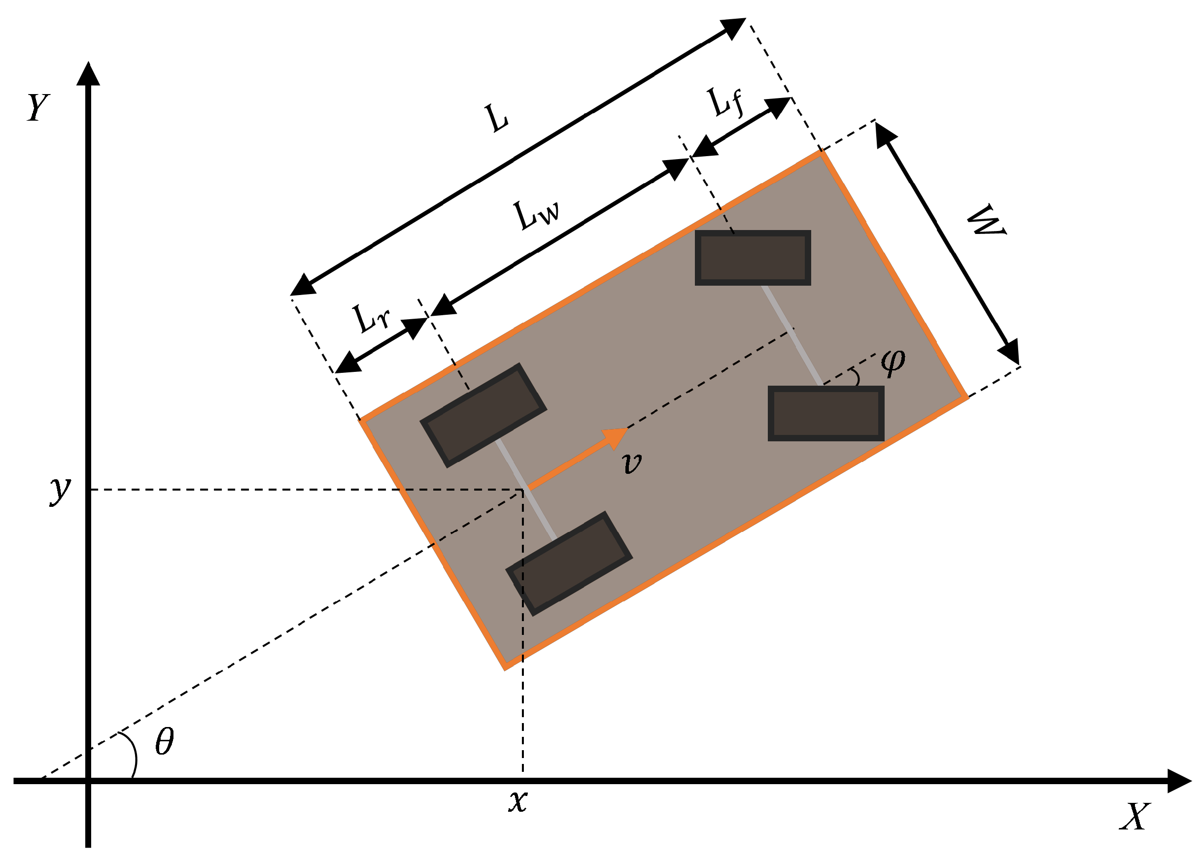The total number of trajectory points is denoted by n. Some geometric and kinematic parameters of the vehicle are illustrated in Figure 3, in which L denotes the vehicle length, $L_f$ denotes the length of the front overhang, $L_r$ denotes the length of the rear overhang, $L_w$ denotes the length of the wheelbase, and W denotes the vehicle width.

The framework of the trajectory planning method proposed in this article is shown in Figure 4, which includes two modules: trajectory generation and trajectory optimization. The trajectory generation module uses the DS-MPT method to calculate the trajectory, including full state variables with a fixed time resolution. Subsequently, the trajectory resampling module fine-tunes the trajectory in the time dimension, leaving enough time for forward and backward movement switching and steering-angle transformation. At the same time, the initial value of the control variable $\left\{a\left(t_i\right),\omega \left(t_i\right)\mid i=1,\dots ,n\right\}$ is calculated through time differentiation. Finally, we design a trajectory optimization module with an improved driving corridor generation method. The trajectory generation method is described in Section 4, and the details of the trajectory optimization method are described in Section 5.

4. Dual-Stage Motion Pattern Tree

In this paper, we propose a joint spatial–temporal trajectory generation method called dual-stage motion pattern tree (DS-MPT). In DS-MPT, the trajectory generation problem is modeled as a multi-step motion pattern decision problem. A discrete state variable set ($Z=\left\{z\left(t_i\right)\right|i=1\dots n\}$) and action variable set ($M=\left\{m\left(t_i\right)\right|i=1\dots n-1\}$) are used to represent the trajectory of the vehicle from the initial state to the target state. $z\left(t_i\right)=\left[{x(t}_i\right),{y(t}_i),{\theta (t}_i\left)\right]$ represents the pose of the vehicle at the end of each decision-making step. $m\left(t_i\right)=m_k$ represents the action performed during $t_i$ and $t_{i+1}$, which is set to six fixed motion patterns.

In the solution process, the first step is to standardize the problem by primarily converting the coordinates of the map elements and aligning the target state with the coordinate origin [0, 0, 0], thereby improving data stability. Secondly, irrespective of the pull-in or pull-out process, DS-MPT leverages the end posture within the parking lot as the initial state. This choice offers several advantages. Firstly, it facilitates the definition of the transition from the posture adjustment stage to the merging stage. Additionally, the collision probability of the Reeds–Shepp curve in the merging stage is lower, which is beneficial to improve the solution efficiency. However, in the case of the pull-in process, this approach leads to a reversed trajectory. Nevertheless, we can rectify this by reversing the order of trajectory nodes and adjusting the direction of $v\left(t_i\right)$ to obtain the correct trajectory.

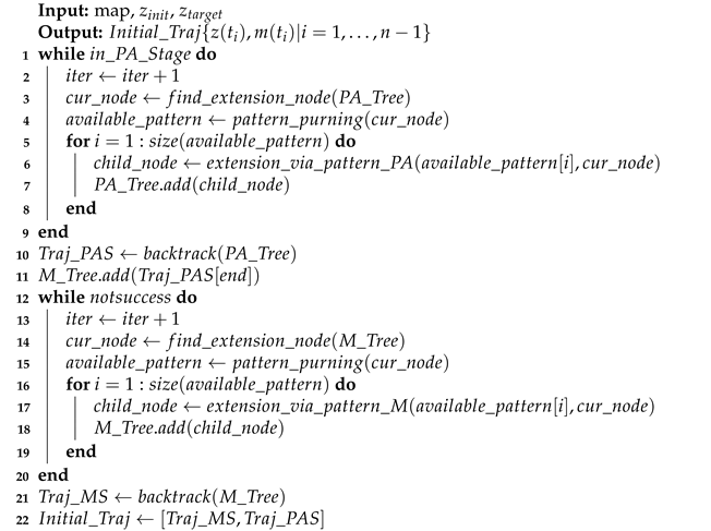
The complete algorithm flow is illustrated in Algorithm 1. The algorithm consists of two stages: lines 1–10 for the posture adjustment stage and lines 11–21 for the merging stage. The trajectory expansion in each stage includes three main functions: optimal node selection (lines 3 and 14), motion pattern pruning (lines 4 and 15), and trajectory tree extension (lines 6 and 17).

Algorithm 1: Dual-Stage Motion Pattern Tree

4.1. Trajectory Tree Extension via Motion Pattern

We define $M=\{SF,SB,LF,RF,LB,RB\}$ as the set of motion patterns that the vehicle may choose at each step ($t_i$), representing moving straight forward, moving straight backward, left turning forward, right turning forward, left turning backward, and right turning backward, respectively. Each movement pattern ($m_k$) is given a unique speed ($v_k$) and front-wheel angle value (${\phi }_k$). The state transition function ($P\left({z(t}_i),m_k^i\right)\to {\mathbb{R}}^3$) for the trajectory generation problem is shown in (2). In order to prioritize solution efficiency, the constraints of acceleration (a) and angular velocity ($\omega$) are disregarded in this process.

$$\left[\begin{array}{c}x\left(t_{i+1}\right)\hfill \\ y\left(t_{i+1}\right)\hfill \\ \theta \left(t_{i+1}\right)\hfill \end{array}\right]=\left[\begin{array}{c}cos\left({\theta }_i\right)\times v_k^i\\ sin\left({\theta }_i\right)\times v_k^i\\ tan\left({\phi }_k^i\right)\times v_k^i/L_w\end{array}\right]\mathrm{\Delta }t+\left[\begin{array}{c}x\left(t_i\right)\hfill \\ y\left(t_i\right)\hfill \\ \theta \left(t_i\right)\hfill \end{array}\right],$$

(2)

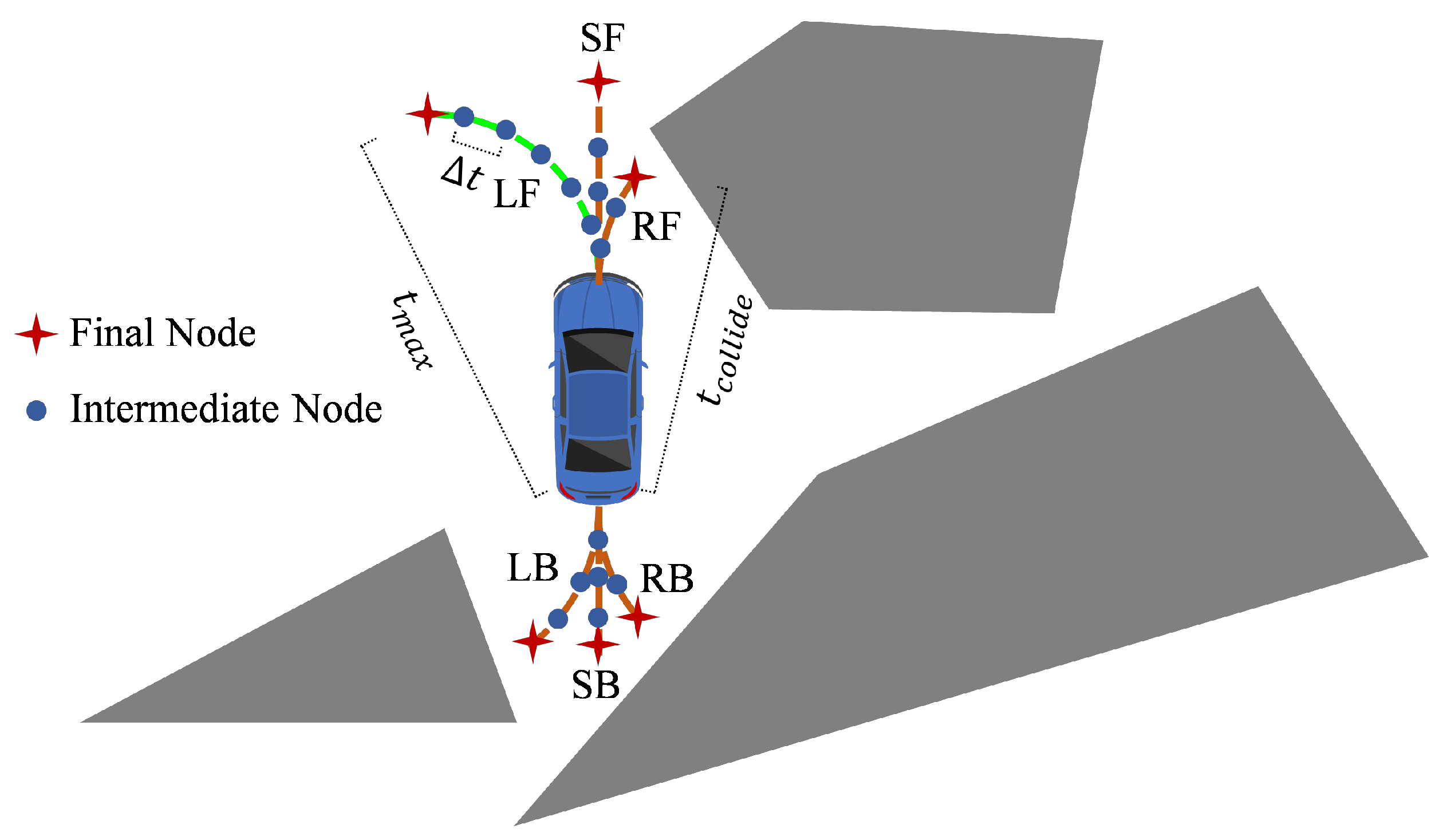
In each decision-making step, the execution time of each $m_k^i$ can be calculated by $t_k^i=min(t_{max},t_{collide})$. Where $t_{max}$ is a preset hyperparameter that specifies the maximum expansion time of the motion pattern and $t_{collide}$ refers to the minimum time required to collide with an obstacle when expanding under $m_k^i$. It is important to note that this method does not add a node to the trajectory tree after each forward simulation step via $▵t$. Instead, it only adds the final expanded node within each motion pattern via $t_k^i$, as shown in Figure 5. When a node is selected as an expansion node, the intermediate nodes are re-introduced into the trajectory to enhance its time resolution. Unlike the interpolation encrypted method, the intermediate nodes undergo collision detection, providing a stronger safety guarantee. In this article, $t_{max}$ is set to 1 s, and $▵t$ is set to 0.05 s.

Another important consideration during the expansion process is determining the criteria for exiting the posture adjustment stage. This article provides a determination formula based on the difference between the heading angle of the extended node (${\theta }_{ex}$) and the heading angle of the terminal state in the parking space (${\theta }_{ter}$):

$$in\_PA=\left\{\begin{array}{cc}1,& if\left|{\theta }_{ex}-{\theta }_{ter}\right|\le {\epsilon }_{\theta }\\ 0,& else\end{array}\right.,$$

(3)

where ${\epsilon }_{\theta }$ is a predefined hyperparameter that refers to the angle threshold used to switch the planning stage. The trajectory tree is expanded with the terminal state in the parking space as the initial node, so ${|\theta }_{ex}-{\theta }_{ter}|=0$ in initial. In the posture adjustment stage, we select the node whose heading angle is biased towards the direction of the ${\theta }_{ter}$-normal vector as the expansion node. As a result, the difference between ${\theta }_{ex}$ and ${\theta }_{ter}$ gradually increases until it surpasses the specified threshold (${\epsilon }_{\theta }$). At that point, the extension process is considered to have completed the posture adjustment stage and transitioned into the merging stage. In this article, ${\epsilon }_{\theta }$ is set to $\pi /4$.

The selection range for expansion nodes in each round does not include the entire trajectory tree but only the children nodes expanded in the previous round. Additionally, the relationship between children and parent nodes is determined strictly based on the expansion steps.

4.2. Node Evaluation

This paper introduces two heuristic cost functions for evaluating motion patterns in the merging stage and posture adjustment stage. In the merging stage, the heuristic calculates the non-holonomic kinematic distance to the end state, which is approximated using the length of the RS curve [46]. In the posture adjustment stage, the heuristic is determined by the angle between the current vehicle heading and the normal vector of the target-state heading.

$$\begin{array}{c}\hfill h\left(z\left(t_{i-1}\right),m_k^i\right)=\left\{\begin{array}{c}L\left(RS\left(z\left(t_i\right),z_{\mathrm{tar}}\right)\right)\hfill \\ arccos\left(I\left(\theta \left(t_i\right)\right)·\overline{I}\left({\theta }_{\mathrm{tar}}\right)/\mid I\left(\theta \left(t_i\right)|\times |\overline{I}\left({\theta }_{\mathrm{tar}}\right)\mid \right)\right.\hfill \end{array}\right.\end{array}$$

(4)

where $RS(z\left(t_i\right),z_{tar})$ represents the Reeds–Shepp curve between $z\left(t_i\right)$ and $z_{tar}$, $L(·)$ represents the length of the curve, $I\left(\theta \right)$ represents the unit direction vector corresponding to $\theta$, and $\overline{I}$ represents the normal vector of I.

4.3. Tree Pruning Strategy

As shown in Figure 6, this paper prunes the trajectory tree by removing invalid motion patterns. Three situations are considered. Firstly, when $z\left(t_i\right)$ is extended from $m_k^{i-1}$ and $t_k^{i-1}<t_{max}$, the optimal motion pattern in $z\left(t_{i-1}\right)$ is extended until it collides with an obstacle. If $z\left(t_i\right)$ continues to expand in motion mode $m_k^{i-1}$, it will be invalid. Secondly, the motion patterns in M are opposite movements to each other, $SF$ and $SB$ are opposite movements to each other, and $LF$ and $LB$ are opposite movements to each other, as are $RF$ and $RB$. Let $(m_k^{i-1},{\tilde{m}}_k^{i-1})$ represent a pair of reverse motion patterns. If state $z\left(t_i\right)$ is expanded from $z\left(t_{i-1}\right)$ via $m_k^{i-1}$, then $z\left(t_i\right)$ has a greater probability returning to $z\left(t_{i-1}\right)$ if it continues to expand via ${\tilde{m}}_k^{i-1}$. The trajectory tree pruning strategy is expressed by the following formula:

$$M_k^i=\left\{\begin{array}{c}M-{\tilde{m}}_k^{i-1},t_k^{i-1}=t_{max}\\ M-\left\{{\tilde{m}}_k^{i-1},m_k^{i-1}\right\},t_k^{i-1}<t_{max}\end{array}\right.$$

(5)

$$k=\underset{k}{argminh}\left(z\left(t_{i-1}\right),m_k^{i-1}\right)$$

(6)

Thirdly, during motion pattern tree expansion in the merging stage, each step expansion attempts to establish a connection with the end node using the RS curve. If the connected curve does not result in a collision, the initial trajectory is considered successfully generated.

4.4. Collision Detection

The geometric space is denoted as ${\rm Y}$, the obstacle space as ${{\rm Y}}_{obs}\subset {\rm Y}$, and the available geometric space as ${{\rm Y}}_{ava}={\rm Y}\setminus {{\rm Y}}_{obs}$. In the trajectory generation process, obstacles are expressed in the form of a grid map, and the obstacle constraints are expressed as follows:

$${{\rm Y}}_v\left(z\left(t_i\right)\right)\cap {{\rm Y}}_{obs}=\varnothing ,\forall iϵ\{1,\dots ,n\}$$

(7)

where ${{\rm Y}}_v\left(z\left(t_i\right)\right)$ represents the grid occupied by the vehicle envelope at time $t_i$.

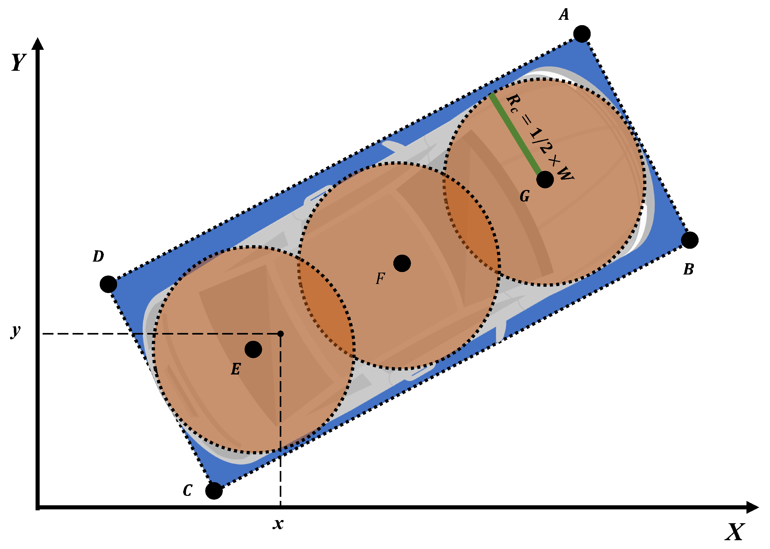
In the parallel parking task, the vehicle envelope’s corner points are prone to collisions. Using an approximate representation that ignores the corner points (e.g., inscribed circles) reduces computational complexity but simultaneously compromises the quality of the solution. Considering calculation efficiency and detection accuracy, this paper combines two envelope forms, namely disk approximations and an oriented bounding box (OBB), to simplify the representation of the vehicle shape. we sampled the four corner points of the OBB and the three disk center points. As shown in Figure 7, A, B, C, and D perform collision detection in the original obstacle grid map, and E, F, and G perform collision detection in the dilated grid map. $R_c$ represents the radius of the inscribed circles. The coordinate calculation formula for each detection points is expressed as follows:

$$\begin{array}{cc}\hfill & x_A\left(t_i\right)=x\left(t_i\right)+\left(L_f+L_w\right)\times cos\theta \left(t\right)-1/2\times W\times sin\theta \left(t_i\right)\hfill \\ \hfill & y_A\left(t_i\right)=y\left(t_i\right)+\left(L_f+L_w\right)\times sin\theta \left(t\right)+1/2\times W\times cos\theta \left(t_i\right)\hfill \\ \hfill & x_B\left(t_i\right)=x\left(t_i\right)+\left(L_f+L_w\right)\times cos\theta \left(t\right)+1/2\times W\times sin\theta \left(t_i\right)\hfill \\ \hfill & y_B\left(t_i\right)=y\left(t_i\right)+\left(L_f+L_w\right)\times sin\theta \left(t\right)-1/2\times W\times cos\theta \left(t_i\right),\hfill \\ \hfill & x_C\left(t_i\right)=x\left(t_i\right)-L_r\times cos\theta \left(t_i\right)+1/2\times W\times sin\theta \left(t_i\right),\hfill \\ \hfill & y_C\left(t_i\right)=y\left(t_i\right)-L_r\times sin\theta \left(t_i\right)-1/2\times W\times cos\theta \left(t_i\right),\hfill \\ \hfill & x_D\left(t_i\right)=x\left(t_i\right)-L_r\times cos\theta \left(t_i\right)-1/2\times W\times sin\theta \left(t_i\right),\hfill \\ \hfill & y_D\left(t_i\right)=y\left(t_i\right)-L_r\times sin\theta \left(t_i\right)+1/2\times W\times cos\theta \left(t_i\right),\hfill \\ \hfill & x_E\left(t_i\right)=x\left(t_i\right)+\left(R_c-L_r\right)\times cos\theta \left(t_i\right),\hfill \\ \hfill & y_E\left(t_i\right)=y\left(t_i\right)+\left(R_c-L_r\right)\times sin\theta \left(t_i\right),\hfill \\ \hfill & x_F\left(t_i\right)=x\left(t_i\right)+\left(1/2\times L-L_r\right)\times cos\theta \left(t_i\right),\hfill \\ \hfill & y_F\left(t_i\right)=y\left(t_i\right)+\left(1/2\times L-L_r\right)\times sin\theta \left(t_i\right),\hfill \\ \hfill & x_G\left(t_i\right)=x\left(t_i\right)+\left(L-R_c-L_r\right)\times cos\theta \left(t_i\right),\hfill \\ \hfill & y_G\left(t_i\right)=y\left(t_i\right)+\left(L-R_c-L_r\right)\times sin\theta \left(t_i\right)\hfill \end{array}$$

(8)

The above text presents the core content of the DS-MPT algorithm. Once the trajectory tree is constructed for each stage, the initial trajectory can be obtained through backtracking, and the final trajectory can be obtained by concatenating the trajectories from both stages.

4.5. Trajectory Resample

The trajectory computed by DS-MPT incorporates state quantities ($v\left(t_i\right)$ and $\phi \left(t_i\right)$). However, due to the omission of acceleration and angular velocity constraints, abrupt changes occur in both $v\left(t_i\right)$ and $\phi \left(t_i\right)$. To mitigate this issue, we employ a trajectory resampling strategy. The central approach of resampling is re-planning of the velocity profile. We formulate the issue as a quadratic programming (QP) problem.

The initial trajectory is divided into several segments according to the gear switching. Each segment of the initial trajectory is represented by the following multi-segment n-order polynomial:

$$s\left(t\right)=\left\{\begin{array}{c}\left[1,t,t^2,\dots ,t^n\right]·p_1,t_0\le t\le t_1\hfill \\ \left[1,t,t^2,\dots ,t^n\right]·p_2,t_1\le t\le t_2\hfill \\ \cdots \hfill \\ \left[1,t,t^2,\dots ,t^n\right]·p_m,t_{m-1}\le t\le t_m\hfill \end{array}\right.$$

(9)

In the formula, m is the number of segments of the trajectory curve, and $p_i={[p_{i0},p_{i1},\dots ,p_{in}]}^T$ is the parameter vector of the n-th polynomial curve. Then, the velocity ($v\left(t\right)$), acceleration ($a\left(t\right)$), and jerk ($j\left(t\right)$) of the trajectory point can be expressed as follows:

$$v\left(t\right)=\left\{\begin{array}{c}\left[0,1,2t,\dots ,n{t}^{n-1}\right]·p_1,t_0\le t\le t_1\hfill \\ \left[0,1,2t,\dots ,n{t}^{n-1}\right]·p_2,t_1\le t\le t_2\hfill \\ \cdots \hfill \\ \left[0,1,2t,\dots ,n{t}^{n-1}\right]·p_m,t_{m-1}\le t\le t_m\hfill \end{array}\right.$$

(10)

$$a\left(t\right)=\left\{\begin{array}{c}\left[0,0,2,\dots ,n(n-1)t^{n-2}\right]·p_1,t_0\le t\le t_1\hfill \\ \left[0,0,2,\dots ,n(n-1)t^{n-2}\right]·p_2,t_1\le t\le t_2\hfill \\ \cdots \hfill \\ \left[0,0,2,\dots ,n(n-1)t^{n-2}\right]·p_m,t_{m-1}\le t\le t_m\hfill \end{array}\right.$$

(11)

$$j\left(t\right)=\left\{\begin{array}{c}\left[0,0,0,\dots ,{\displaystyle \frac{n!}{(n-3)!}}{t}^{n-3}\right]·p_1,t_0\le t\le t_1\hfill \\ \left[0,0,0,\dots ,{\displaystyle \frac{n!}{(n-3)!}}{t}^{n-3}\right]·p_2,t_1\le t\le t_2\hfill \\ \cdots \hfill \\ \left[0,0,0,\dots ,{\displaystyle \frac{n!}{(n-3)!}}{t}^{n-3}\right]·p_m,t_{m-1}\le t\le t_m\hfill \end{array}\right.$$

(12)

$s\left(t_{m-1}\right)$ and $s\left(t_m\right)$ are given by the initial trajectory. Since the vehicle switches gears at the end of the trajectory segment, $v\left(t_m\right)$ and $a\left(t_m\right)$ are set to zero. The continuity of $s\left(t\right)$, $\dot{s}\left(t\right)$, $\ddot{s}\left(t\right)$, and $\stackrel{⃛}{s}\left(t\right)$ constitutes equality constraints. At the same time, $v\left(t\right)$ and $a\left(t\right)$ must meet the vehicle motion restrictions in (22). Based on the above analysis, this paper models speed planning as a QP problem:

$$min{\int }_0^T\left({\left(j\left(t\right)\right)}^2+{(v\left(t\right)-v_{max})}^2\right)dt$$

(13)

$$s.t.\left\{\begin{array}{c}{A}_{eq}p=b_{eq}\hfill \\ A_{ieq}p\le b_{ieq}\hfill \end{array}\right.$$

(14)

where $p=[p_1,p_2,\dots ,p_m]$, $A_{eq}$, $b_{eq}$, $A_{ieq}$, $b_{ieq}$ is the parameter of the equality and inequality constraints proposed above.

In solving the aforementioned problem, it is necessary to provide the predetermined execution time (T) for each trajectory segment. As described in Section 3, in the posture adjustment stage, the trajectory segments are typically short in distance, and adjusting the steering wheel angle can be more time-consuming than longitudinal travel. Therefore, we use the following function to schedule execution time:

$$T=max(T_l,T_s)$$

(15)

$$T_l=N_1\ast \sqrt{2s/a_{max}}$$

(16)

$$T_s=N_2\ast \sum \mathrm{\Delta }\phi /{\omega }_{max}$$

(17)

where $T_l$ represents the time required for longitudinal movement and $T_s$ represents the time required to complete front-wheel angle adjustment. $\sum \mathrm{\Delta }\phi$ represents the total steering-angle change during the trajectory segment. $N_1$ and $N_2$ are relaxation factors.

5. Trajectory Optimization

5.1. Trajectory Optimization Problem Definition

In this section, the vehicle state quantities are defined as $z\left(t\right)$, and the vehicle control quantities are defined as $u\left(t\right)$. The relationship between $z\left(t\right)$ and $u\left(t\right)$ can be described by the following differential equation: $\dot{z}\left(t\right)=f(z\left(t\right),u\left(t\right),t)$. The vehicle’s occupation of the geometric space at time t is defined as ${{\rm Y}}_{z\left(t\right)}$. The goal of trajectory optimization is to find the optimal state sequence ($z^{\ast }=[z\left(t_0\right),z\left(t_1\right),\dots ,z\left(t_n\right)]$) and corresponding control sequence ($u^{\ast }=[u\left(t_0\right),u\left(t_1\right),\dots ,u\left(t_n\right)]$) that will avoid collision with obstacles and achieve the minimum value of the objective function. $t_f$ represents the completion time of the entire parking process. The trajectory optimization problem is formulated as follows:

$$\underset{z\left(t\right),u\left(t\right)}{min}J(z\left(t\right),u\left(t\right))$$

(18)

$$s.t.\left\{\begin{array}{c}{Y}_{z\left(t\right)}\subset Y_{ava},\hfill \\ \dot{z}\left(t\right)=f(z\left(t\right),u\left(t\right),t),\hfill \\ z_{min}\le z\left(t\right)\le z_{max},u_{min}\le u\left(t\right)\le u_{max},\hfill \\ z\left(0\right)=z_{init},u\left(0\right)=u_{init},\hfill \\ g_{end}(z\left(t_f\right),z_{end},ϵ)\le 0,u\left(t_f\right)=u_{end},\hfill \\ t\in [0,t_f].\hfill \end{array}\right.$$

(19)

5.2. Objective Function

The objective function of trajectory optimization indicates the expectations for parking efficiency and comfort. In this article, the objective function is defined as follows:

$$J(z\left(t_i\right),u\left(t_i\right))=\sum _{i=1}^n\left|\right|u\left(t_i\right){\left|\right|}^2+\sum _{i=1}^n\left|\right|z\left(t_i\right)-z_{init}\left(t_i\right){\left|\right|}^2$$

(20)

where $z_{init}\left(t_i\right)$ refers to the initial trajectory points calculated by DS-MPT. The objective function comprises two components. The first component aims to minimize the acceleration and front-wheel steering speed during the parking process. The second component aims to maximize the proximity of the optimized trajectory to the initial trajectory.

5.3. Constraints

5.3.1. Kinematic Equality Constraints

Since the parking process is a low-speed movement, we use a discretization kinematic single-track model [47] to describe the equality constraints ($\dot{z}\left(t\right)=f(z\left(t\right),u\left(t\right),t)$) in (19).

$$\left[\begin{array}{c}x\left(t_{i+1}\right)-x\left(t_i\right)\\ y\left(t_{i+1}\right)-y\left(t_i\right)\\ v\left(t_{i+1}\right)-v\left(t_i\right)\\ \phi \left(t_{i+1}\right)-\phi \left(t_i\right)\\ \theta \left(t_{i+1}\right)-\theta \left(t_i\right)\end{array}\right]=\left[\begin{array}{c}\mathrm{\Delta }{t}_o·v\left(t_i\right)·cos\theta \left(t_i\right)\\ \mathrm{\Delta }{t}_o·v\left(t_i\right)·sin\theta \left(t_i\right)\\ \mathrm{\Delta }{t}_o·a\left(t_i\right)\\ \mathrm{\Delta }{t}_o·\omega \left(t_i\right)\\ \mathrm{\Delta }{t}_o·v\left(t_i\right)·tan\phi \left(t_i\right)/L_w\end{array}\right]$$

(21)

where $\mathrm{\Delta }{t}_o$ defines the time interval of the trajectory optimization process.

5.3.2. Kinematic Inequality Constraints

The mechanical characteristics of the vehicle limit the range of state variables and control variables. The relevant constraints( $z_{min}\le z\left(t\right)\le z_{max}$ and $u_{min}\le u\left(t\right)\le u_{max}$) after discretization are expressed as follows:

$$\left[\begin{array}{c}{a}_{min}\\ v_{min}\\ {\omega }_{min}\\ {\phi }_{min}\end{array}\right]\le \left[\begin{array}{c}a\left(t_i\right)\\ v\left(t_i\right)\\ \omega \left(t_i\right)\\ \phi \left(t_i\right)\end{array}\right]\le \left[\begin{array}{c}{a}_{max}\\ v_{max}\\ {\omega }_{max}\\ {\phi }_{max}\end{array}\right]$$

(22)

5.3.3. Boundary Value Constraints

The boundary value constraints are implemented to ensure that the starting and ending nodes of the trajectory meet the requirements of the planning task. The starting-point constraints ($z\left(0\right)=z_{init},u\left(0\right)=u_{init}$) are expressed as follows:

$$[x\left(t_0\right),y\left(t_0\right),\theta \left(t_0\right),v\left(t_0\right),\phi \left(t_0\right),a\left(t_0\right),\omega \left(t_0\right)]=[x_{init},y_{init},{\theta }_{init},v_{init},{\phi }_{init},a_{init},{\omega }_{init}]$$

(23)

The constraints on the trajectory’s end node differ from those on the start node. Firstly, a slight deviation from the target state is permitted for the end state, which facilitates the solving process. Secondly, in order to avoid incorrectly fixing the phase difference between $\theta \left(t_0\right)$ and $\theta \left(t_n\right)$, the constraints of $\theta \left(t_n\right)$ refer to the construction method proposed in [27].

$$[v\left(t_n\right),\phi \left(t_n\right),\alpha \left(t_n\right),\omega \left(t_n\right)]=[v_{end},{\phi }_{end},a_{end},{\omega }_{end}],$$

(24)

$$\left[\begin{array}{c}x\left(t_n\right)-x_{end}\\ y\left(t_n\right)-y_{end}\end{array}\right]\le \left[\begin{array}{c}{ϵ}_x\\ {ϵ}_y\end{array}\right],$$

(25)

and

$$sin\theta \left(t_n\right)=sin{\theta }_{end}cos\theta \left(t_n\right)=cos{\theta }_{end}$$

(26)

5.3.4. Collision Avoidance Constraints

In trajectory optimization, obstacles avoidance constraints are implicitly enforced by confining trajectory nodes within specified driving corridors:

$$\begin{array}{cc}& x_{min}^{t_i,j}\le x^j\left(t_i\right)\le x_{max}^{t_i,j}\hfill \\ & y_{min}^{t_i,j}\le y^j\left(t_i\right)\le y_{max}^{t_i,j},\forall iϵ\{1,\dots ,n\},\forall jϵ\{1,\dots ,k\}\hfill \end{array}$$

(27)

where k represents the number of key points on the vehicle envelope for collision detection.

Driving corridors build boxes along each discrete point. The box generation method is the same as that reported in [48]. Since the generation of boxes requires polling and expansion in all directions at specified steps, it is time-consuming. As described in Section 3, the vehicle pose in the posture adjustment stage is usually located in the same rectangular area. Therefore, we pre-generate a bounding box around the parking plot with the target position as the center. Before polling and expansion, the algorithm first determines whether the envelope sampling points are all located within this rectangular area. If the conditions are met, the bounding box is directly used as a constraint to avoid repeated generation. Detailed calculation steps are illustrated in Algorithm 2.

Algorithm 2: Enhanced Driving Corridor Generation Algorithm

6. Experimental Setups, Results, and Analysis

6.1. Experimental Scenarios and Parameters

The simulation experiments were conducted in Matlab R2020b and executed on an AMD Ryzen 9 4900HS CPU with 16 GB RAM. The trajectory optimization problem defined in our method is solved by IPOPT through the AMPL interface. The parameters used in this experiment are shown in

Table 1. Experimental Parameters.

Symbol	Vehicle Geometry Parameter Description	Unit	Value
$L_w$	Wheelbase	m	2.8
$L_f$	Front overhang length	m	0.96
$L_r$	Rear overhang length	m	0.929
W	Vehicle width	m	1.942
L	Vehicle length	m	4.689
Symbol	Grid-Map Parameter Description	Unit	Value
$X_{min},X_{max}$	X-dimension range	m	[−20, 20]
$Y_{min},Y_{max}$	Y-dimension range	m	[−20, 20]
$X_{\mathrm{res}}$	X-dimension resolution	m	0.05
$Y_{\mathrm{res}}$	Y-dimension resolution	m	0.05
Symbol	Vehicle Kinematic Parameter Description	Unit	Value
$v_{max}$	Maximum velocity	m/s	1.5
$a_{max}$	Maximum acceleration	m/s2	1.0
${\phi }_{max}$	Maximum steering angle	rad	0.75
${\omega }_{max}$	Maximum angular velocity	rad/s	0.5
$\mathrm{\Delta }{t}_g$	Time sampling resolution in trajectory generation	s	0.05
${\mathrm{t}}_{max}$	Maximum sampling time	s	1.0
${\epsilon }_{\theta }$	Threshold for the stage change	rad	$\pi$/4
${\mathrm{N}}_1$	Relaxation factor of ${\mathrm{T}}_l$	∖	5.0
${\mathrm{N}}_2$	Relaxation factor of ${\mathrm{T}}_s$	∖	2.0
$\mathrm{\Delta }{t}_o$	Time sampling resolution in trajectory optimization	s	0.2
$\mathrm{\Delta }l$	Expansion step size of box	m	0.1
${\mathrm{l}}_{max}$	Maximum expansion length of box	m	5.0
${ϵ}_x$	Boundary value relaxation on the x-axis	m	0.1
${ϵ}_y$	Boundary value relaxation on the y-axis	m	0.1

.

This paper conducts simulation experiments in sixteen parallel parking scenarios. Among them, Cases 1–6 are derived from the typical parallel parking scenes provided in the Trajectory Planning Competition for Automated Parking (TPCAP) [49]. Cases 7–11 represent typical parallel parking scenarios with narrow passages, where the passage widths are 4.667 m, 4.278 m, 3.890 m, 3.501 m, and 3.113 m, respectively. Cases 12–16 are typical parallel parking scenes with a narrow lot area in which the length ranges of the parking lot are 5.639 m, 5.546 m, 5.452 m, 5.358 m, and 5.264 m, respectively. The experiments are divided into four parts. Firstly, comparative experiments are conducted to evaluate different trajectory generation methods. Secondly, the effectiveness of the enhanced driving corridor generation method is demonstrated through experiments. Thirdly, comparative experiments are conducted to demonstrate the superiority of our method over different trajectory planning methods. Finally, to evaluate the robustness of our method, we conduct experiments with randomly sampled initial states in Case 16 and introduce random obstacles in Case 6.

6.2. Experiments for Trajectory Generation Methods

In this section, this paper selects CPU time ($T_i$), the number of solution iterations ($N_i$), trajectory length ($L_i$), the number of switching maneuvers ($N_v$), and point density ($D_p$) as evaluation metrics. We selected Fault-tolerant Hybrid A* (FTHA) for comparison, which was proposed in [27] and enhances the completeness of the Hybrid A* method. Another comparison method is based on a spatial–temporal decomposition strategy (STD) [45]. STD uses the two-stage characteristics of parallel parking like DS-MPT. The difference is that STD is solved based on the optimization method, while DS-MPT is based on the sampling and searching method. STD relies on structured scene descriptions and is not applicable to unstructured scenes in TPCAP cases. Therefore, in Case 1 to Case 6, we only compare the FTHA method with the DS-MPT method. In Case 7 to Case 16, we uniformly compare the performance of the three methods.

The corresponding statistical indicators are summarized in

Table 2. Experimental results for trajectory generation methods.

Case	Method	${\mathit{T}}_{\mathit{i}}$ (s)	${\mathit{N}}_{\mathit{i}}$	${\mathit{L}}_{\mathit{i}}$ (m)	${\mathit{N}}_{\mathit{v}}$	${\mathit{D}}_{\mathit{p}}$
1	FTHA	0.103	6	11.837	2	2.619
	DS-MPT	0.234	7	13.604	3	8.527
2	FTHA	0.650	64	12.074	2	3.644
	DS-MPT	0.069	4	9.657	3	8.388
3	FTHA	3.006	501	8.389	1	0.954
	DS-MPT	0.183	8	7.651	4	10.587
4	FTHA	0.302	26	14.652	2	2.389
	DS-MPT	0.170	8	15.681	3	8.099
5	FTHA	0.722	54	16.114	2	2.669
	DS-MPT	0.251	7	16.938	2	8.383
6	FTHA	0.695	69	17.665	6	1.359
	DS-MPT	0.187	7	17.704	4	8.303
	STD	8.787	1694	16.919	3	4.728
7	FTHA	1.157	65	17.616	6	1.362
	DS-MPT	0.227	8	16.357	3	8.070
	STD	4.071	989	19.496	1	4.104
8	FTHA	0.631	38	17.625	6	1.362
	DS-MPT	0.164	8	15.996	3	8.002
	STD	10.282	2016	17.49	3	4.574
9	FTHA	0.468	29	16.023	6	1.498
	DS-MPT	0.133	11	16.555	3	8.034
	STD	12.147	3343	17.742	3	4.509
10	FTHA	0.715	54	19.705	5	1.32
	DS-MPT	0.130	9	17.389	3	8.051
	STD	4.45	738	24.944	28	3.207
11	FTHA	4.824	501	17.021	5	1.058
	DS-MPT	0.321	23	18.265	3	8.048
	STD	2.758	566	16.6	3	3.614
12	FTHA	0.538	45	14.569	2	2.54
	DS-MPT	0.241	7	15.748	3	7.938
	STD	2.147	434	21.353	3	2.81
13	FTHA	0.482	45	14.569	2	2.54
	DS-MPT	0.240	8	15.741	3	7.941
	STD	5.367	1312	16.778	3	3.576
14	FTHA	0.460	45	14.569	2	2.54
	DS-MPT	0.207	12	16.209	5	8.082
	STD	10.069	2491	17.121	8	4.673
15	FTHA	0.457	45	14.569	2	2.54
	DS-MPT	0.251	14	16.056	7	8.097
	STD	4.572	1109	17.825	10	4.488
16	FTHA	7.525	151	15.249	4	2.54
	DS-MPT	0.191	16	15.601	11	8.012

, while the planning results of DS-MPT are presented in Figure 8. Across all test scenarios, the DS-MPT method exhibits superior execution efficiency compared to the other methods, except for Case 1. This superiority is evident through $T_i$ and $N_i$. Compared to FTHA, the DS-MPT method exhibits a longer CPU time per iteration (DS-MPT: 0.022 vs. FTHA: 0.015) due to the necessity of multiple high-resolution sampling and collision detection executions. Nonetheless, with the aid of precise two-stage heuristic information and efficient tree pruning strategies, DS-MPT achieves more accurate selection of expansion nodes. Consequently, it demands fewer iterations, thereby establishing an advantage in terms of execution efficiency. Furthermore, when considering $T_i$ and $N_i$ in different scenarios, the DS-MPT method demonstrates remarkable numerical stability, exhibiting low sensitivity to changes in the number of obstacles and parking space narrowness. The standard variance of $T_i$ and $N_i$ for the entire scenarios is significantly lower for the DS-MPT method compared to FTHA and STD, which can be seen in

Table 3. Metric statistics for trajectory generation experiments.

		STD	FTHA	DS-MPT
$T_i$ (s)	Mean	6.465	1.421	0.200
	Max	12.147	7.525	0.321
	Min	2.147	0.103	0.069
	Std Dev	3.531	2.026	0.060
$N_i$	Mean	1222	59	9
	Max	3343	501	23
	Min	434	6	4
	Std Dev	878.17	151.25	4.461
$D_p$	Mean	3.972	1.914	8.265
	Max	4.728	3.644	10.587
	Min	2.81	0.954	7.938
	Std Dev	0.647	0.75	0.618

.

In terms of trajectory quality metric, the FTHA method performs better. Specifically, FTHA achieves the best $N_v$ index in 9 out of the 16 scenarios. Similarly, in terms of $L_i$, FTHA performs better than other methods in 11 out of the 16 scenes. We analyze the reasons for this result. On one hand, the heuristic function employed by the DS-MPT algorithm during the posture adjustment stage prioritizes the transformation of the vehicle’s heading angle. This, coupled with the node extension strategy relying on collisions with the environment, potentially leads to local optimal solutions in not very narrow scenarios. Additionally, for the sake of completeness, the FTHA method incorporates the A* algorithm to connect the end point when the maximum number of iterations is reached. However, the trajectory generated by A* does not account for vehicle kinematics. As a result, while the FTHA method may exhibit favorable metrics in terms of $N_v$ and $L_i$, its resulting trajectory may deviate further from the true optimal safe trajectory. Figure 9 illustrates the trajectories planned by DS-MPT and FTHA. In Cases 1, 2, and 4, notable differences are observed in the maneuver points generated by the two methods. In Case 3, FTHA reaches the maximum iteration limit and directly connects the target state to the nearest optimal node, potentially violating kinematic and obstacle constraints. Compared with the STD method, it can be found that the trajectory length generated by DS-MPT is relatively close to the trajectory length calculated by STD, and the length of the former is always slightly shorter than that of the latter. In terms of $N_v$, DS-MPT achieves performance better than or equal to that of STD in 70% of scenarios.

Another noteworthy metric is the density of trajectory points. As shown in Table 2 and Table 3, the DS-MPT method not only exhibits superior solving efficiency but also achieves a higher density of trajectory points, averaging eight points per meter. It is important to emphasize that the higher trajectory-point density in DS-MPT is not attained through simple interpolation. Rather, collision detection is performed for each node in the trajectory, ensuring a more reliable and safer trajectory. However, FTHA and STD can also improve the trajectory point density by adjusting parameters, for example, by choosing a smaller expansion step size for the FTHA method or increasing the number of optimized subsequences for the STD method, although this means a longer solution time.

6.3. Experiments for Enhanced Driving Corridors Generation Strategy

We measure the computational efficiency of the two driving corridor generation strategies. The origin corridor generation method is cited from [48]. The experiment assesses the utilization of the original method for generating driving corridors with three inner-circle center points, as well as the utilization of both the original strategy and the enhanced strategy for generating driving corridors with seven envelope sampling points. The experimental results are shown in Figure 10. When generating corridors for seven sampling points, the enhanced strategy can significantly reduce the calculation time by 54–84% compared to the original strategy. Importantly, the calculation time is lower than or comparable to that of the original method, which calculates the driving corridor using three inner-circle center points.

6.4. Experiments for Trajectory Planning Methods

We compared our proposed trajectory planning method with the approaches presented in [27,30,45]. The method proposed in [27] utilizes the aforementioned FTHA method for trajectory discovery and introduces a lightweight iterative framework called LIOM. In LIOM, the nonlinear equalities in the optimization problem are softened using external penalty functions and incorporated into the objective function. An iterative update strategy for driving corridors is additionally adopted. This method demonstrates strong advantages in terms of algorithmic execution efficiency and completeness. The STD method proposed in [45] uses the two-stage characteristics as a kind of expert knowledge to reduce the complexity of obstacle avoidance constraints, with a high solution success rate in narrow scenarios. The H-OBCA method proposed in [30] proposes a method to accurately model obstacle constraints without approximation errors caused by driving corridors. Therefore, H-OBCA has great potential in narrow scenarios. We compare above methods and our method in Case 7 to Case 16.

The experimental results are shown in

Table 4. Experimental results for trajectory planning methods.

Case	Method	${\mathit{T}}_{\mathit{i}}$ (s)	${\mathit{T}}_{\mathit{o}}$ (s)	${\mathit{N}}_{\mathit{o}}$	${\mathit{L}}_{\mathit{o}}$ (m)	${\mathit{N}}_{\mathit{v}}$
7	FTHA + LOAM	0.874	0.797	240	18.662	4
	STD	8.787	0.451	103	16.967	3
	H-OBCA	1.112	1.584	116	21.73	2
	DS-MPT + NLP	0.230	1.054	27	17.428	2
8	FTHA + LOAM	1.119	0.801	249	17.931	9
	STD	4.071	0.034	7	19.499	1
	H-OBCA	1.087	2.253	174	21.73	2
	DS-MPT + NLP	0.203	1.14	30	17.421	2
9	FTHA + LOAM	1.014	0.794	252	17.729	6
	STD	10.282	0.041	11	17.495	3
	H-OBCA	1.647	1.869	120	21.73	2
	DS-MPT + NLP	0.172	1.506	32	17.781	3
10	FTHA + LOAM	1.269	0.825	244	21.95	8
	STD	12.147	0.598	129	17.747	3
	H-OBCA	1.908	0.886	69	21.73	2
	DS-MPT + NLP	0.163	1.259	29	17.957	3
11	FTHA + LOAM	\	\	\	\	\
	STD	4.45	0.028	7	24.941	28
	H-OBCA	2.073	1.785	124	21.731	3
	DS-MPT + NLP	0.359	1.38	31	19.286	3
12	FTHA + LOAM	1.982	0.823	240	18.267	5
	STD	2.758	0.030	9	16.604	3
	H-OBCA	1.071	0.951	59	21.73	2
	DS-MPT + NLP	0.239	1.182	30	17.241	3
13	FTHA + LOAM	1.929	0.813	241	18.257	5
	STD	2.147	0.038	9	21.405	3
	H-OBCA	1.102	1.881	120	21.73	2
	DS-MPT + NLP	0.288	1.22	32	16.621	3
14	FTHA + LOAM	1.959	0.812	246	18.23	5
	STD	5.367	0.029	11	16.780	3
	H-OBCA	39.448	1.272	69	21.731	5
	DS-MPT + NLP	0.287	6.347	97	17.274	5
15	FTHA + LOAM	1.73	0.829	240	18.034	4
	STD	10.069	0.433	89	18.576	8
	H-OBCA	\	\	\	\	\
	DS-MPT + NLP	0.263	3.839	57	17.043	7
16	FTHA + LOAM	1.7525	0.827	241	18.031	4
	STD	4.572	0.058	13	17.820	10
	H-OBCA	\	\	\	\	\
	DS-MPT + NLP	0.197	8.868	79	18.122	17

and

Table 5. Statistics for trajectory planning experiments.

		FTHA + LIOM	STD	H-OBCA	DS-MPT + NLP
$T_i\left(s\right)$	Mean	1.514	6.465	6.181	0.24
	Max	1.982	12.147	39.448	0.359
	Min	0.874	2.147	1.071	0.163
	Std Dev	0.417	3.35	12.579	0.058
$T_o\left(s\right)$	Mean	0.813	0.174	1.56	2.78
	Max	0.829	0.598	2.253	8.868
	Min	0.794	0.028	0.886	1.054
	Std Dev	0.013	0.214	0.453	2.597
$T_a\left(s\right)$	Mean	2.328	6.639	7.741	3.02
	Max	2.805	12.745	40.72	9.065
	Min	1.671	2.185	2.022	1.284
	Std Dev	0.426	3.52	12.476	2.597
$N_o$	Mean	244	39	107	45
	Max	252	129	174	97
	Min	240	7	59	27
	Std Dev	4.19	45.593	36.031	23.588
$R_s$		90%	100%	80%	100%

, in which $T_i$ represents the time required for initial trajectory generation, $T_o$ represents the time required for trajectory optimization (CPU time in IPOPT), $T_a$ represents a summary of $T_i$ and $T_o$, $N_o$ represents the number of iterations required for trajectory optimization, $L_o$ represents the optimal trajectory length, and $N_v$ represents the number of maneuvers in the optimal trajectory.

In terms of efficiency indexes and success rate, our method performs better than other methods on the $T_i$ index. It not only takes less time, on average, but also shows stronger stability. Furthermore, considering the average total calculation time, our method ranks second after the FTHA + LIOM method. However, it is worth noting that our method exhibits a higher solution success rate compared to FTHA + LIOM. In all cases, both our method and the STD method achieve a 100% solution success rate. We analyze the cases where the solution fails. The main reason for this is either the failure of the initial solution or the unacceptable quality of the initial solution. As a result, the DS-MPT method proposed in this article shows significant potential in enhancing computational efficiency and success rates for other trajectory optimization methods.

In terms of trajectory quality indicators, both the STD method and our method exhibit excellent performance in terms of $L_o$. Our method produces the shortest trajectory in four scenarios, while the STD method outperforms in the remaining six scenarios. For the $N_v$ indicator, there are significant differences among the four methods. The reason is that all the methods used in the experiments transform the continuous-time trajectory planning problem into a finite, nonlinear program with constraints applied at finite collocation points. However, potential violations between adjacent collocation points can occur. Because of this, some trajectories find exactly two feasible collocation points that cross the obstacle. In this situation, although the trajectory has a lower $N_v$ value, it is actually not feasible. To be honest, our method does not solve this problem. However, since the initial speed profile considers the two-stage characteristics, more points in the initial trajectory are concentrated near the parking area. The optimal obtained trajectory is relatively better in terms of safety. Figure 11 shows the trajectories obtained by H-OBCA and our method under Case 12.

In order to further analyze the optimality of the trajectories obtained by our method, we calculate the standard deviations of the differentials of four quantities $\left[v\right(t),\phi (t),a(t),\omega (t\left)\right]$ in the optimal trajectories obtained from three cases, the results of which are shown in

Table 6. Standard deviations of the optimal states/control variables.

Case	${\mathit{v}}_{\mathbf{std}}$	${\mathit{\phi }}_{\mathbf{std}}$	${\mathit{a}}_{\mathbf{std}}$	${\mathit{\omega }}_{\mathbf{std}}$
14	0.0191	0.0338	0.0092	0.0254
15	0.0167	0.0443	0.0091	0.0265
16	0.0165	0.0353	0.0097	0.0342

. Figure 12, Figure 13 and Figure 14 present the curves of state variables and control variables in the optimal trajectories. The results indicate that the optimal trajectories obtained using our method do not exhibit abrupt changes in the state variables $\left[v\right(t),\phi (t\left)\right]$ or control variables $\left[a\right(t),\omega (t\left)\right]$. By comparing the extreme values in the figures, we can conclude that the solved trajectories satisfy the vehicle kinematic constraints stated in Equation (22).

6.5. Robustness Analysis

To further analyze the robustness of the proposed trajectory planning method, we conducted two additional experiments. First, a random experiment was performed for parking Case 16, involving 200 Monte Carlo trials. The initial conditions of the vehicle were varied, with the random initialization data summarized in

Table 7. Stochastic initial state generation parameters.

Initial State	Unit	Distribution	Range
$p_x\left(0\right)$	m	Uniform	$[-8,10]$
$p_y\left(0\right)$	m	Uniform	$[-2.5,4.5]$
$p_{\theta }\left(0\right)$	rad	Uniform	$[0,{\displaystyle \frac{\pi }{2}}]$

. In the second experiment, 20 scenarios were generated based on Case 6 by randomly adding obstacles. The parameters of these random obstacles are detailed in

Table 8. Stochastic obstacles generation parameters.

Random Obstacle	Unit	Distribution	Range
$cente{r}_x$	m	Uniform	$[4,12]$
$cente{r}_y$	m	Uniform	$[4,8]$
$number$	∖	Uniform	$[1,3]$

.

Our four performance indicators are listed in

Table 9. Convergence results with random initial states.

Method	${\mathit{N}}_{\mathit{s}}$	${\mathit{N}}_{\mathit{inf}}$	${\mathit{t}}_{\mathit{a}}$	${\mathit{t}}_{\mathit{s}}$	Success Rate
DS-MPT	200	0	0.0595	0.0852	100%
DS-MPT + NLP	185	15	30.277	16.840	92.5%

: the times of successful solution ($N_s$), the times of infeasible solution ($N_{inf}$), the average total solve time ($t_a$), and the standard deviation of total solve time ($t_s$). The DS-MPT method was successfully solved in all random situations, and the average time consumption was relatively stable, but the success rate of back-end trajectory optimization was reduced. The success rate in 200 experiments was 92.5%, and the standard deviation of the solve time was larger. This is because the trajectories generated by DS-MPT under random conditions have different lengths and the number of trajectory points is also different, leading to uncertainty in the scale of the optimization problem. Longer trajectories increase the size of the optimization variables, prolonging the solution time.

Table 10. Convergence results with random obstacles.

Method	${\mathit{N}}_{\mathit{s}}$	${\mathit{N}}_{\mathit{inf}}$	${\mathit{t}}_{\mathit{a}}$	${\mathit{t}}_{\mathit{s}}$	Success Rate
DS-MPT	20	0	0.227	0.141	100%
DS-MPT + NLP	20	0	1.700	0.778	100%

presents the experimental results under conditions with random obstacles. The algorithm’s success rate and computation time remained consistent despite the increasing complexity of the obstacle distribution, demonstrating strong robustness.

7. Discussion

This paper investigated the problem of trajectory planning under narrow terminal constrains. A novel trajectory generation approach called DS-MPT was structured to plan parking maneuvers with higher computational efficiency and robustness. Subsequently, a trajectory optimization method was introduced, along with an enhanced driving corridor generation strategy.

Based on the experimental simulation results, we found that trajectory planning under narrow terminal constrains has dual-stage characteristics. The heuristic functions designed for the two stages better guide the expansion of the trajectory tree, thereby improving the calculation efficiency. At the same time, the speed re-planning method and the driving corridor generation strategy based on the dual-stage characteristics further improve the trajectory quality, reduce the time consumption of optimization, and improve the success rate of trajectory optimization.

In future work, we will explore strategies to enhance the algorithm’s generalization capabilities, such as by incorporating dual-stage strategies and learning-based techniques. We will also investigate more efficient trajectory optimization methods to reduce computational cost. Furthermore, we aim to develop a general-purpose trajectory planner for unmanned systems operating in narrow, unstructured environments.