Unsupervised Domain Adaptation Semantic Segmentation of Remote Sensing Imagery with Scene Covariance Alignment

Abstract

Remote sensing imagery (RSI) segmentation plays a crucial role in environmental monitoring and geospatial analysis. However, in real-world practical applications, the domain shift problem between the source domain and target domain often leads to severe degradation of model performance. Most existing unsupervised domain adaptation methods focus on aligning global-local domain features or category features, neglecting the variations of ground object categories within local scenes. To capture these variations, we propose the scene covariance alignment (SCA) approach to guide the learning of scene-level features in the domain. Specifically, we propose a scene covariance alignment model to address the domain adaptation challenge in RSI segmentation. Unlike traditional global feature alignment methods, SCA incorporates a scene feature pooling (SFP) module and a covariance regularization (CR) mechanism to extract and align scene-level features effectively and focuses on aligning local regions with different scene characteristics between source and target domains. Experiments on both the LoveDA and Yanqing land cover datasets demonstrate that SCA exhibits excellent performance in cross-domain RSI segmentation tasks, particularly outperforming state-of-the-art baselines across various scenarios, including different noise levels, spatial resolutions, and environmental conditions.

1. Introduction

Remote sensing imagery (RSI) plays a crucial role in numerous environmental monitoring and geospatial analysis applications, including land use classification, urban planning, disaster management, and agricultural monitoring [1,2]. The increasing availability of high-resolution RSI data from satellite and aerial platforms has enhanced our ability to monitor and analyze the Earth’s surface with unprecedented detail. Despite the advantages of high-resolution imagery, inherent variability in image characteristics such as spatial resolution, noise levels, and environmental conditions poses significant challenges for the automatic segmentation and interpretation of remote sensing data [3,4,5].

In recent years, deep learning methods have demonstrated remarkable performance in semantic segmentation of remote sensing imagery, particularly convolutional neural networks (CNNs). These models can automatically learn hierarchical features, ranging from low-level features (such as edges and textures) to high-level semantic features (such as object shapes and regional characteristics), significantly improving segmentation accuracy. However, traditional deep learning methods heavily rely on huge amounts of pixel-level labels [6], which require substantial human effort and time. Moreover, significant variations in data distributions across different regions or within the same region over time or captured by different sensors, as well as factors such as atmospheric effects, cloud cover, and terrain, further increase the complexity of RSI data [7,8]. These challenges often lead to a reduction in model accuracy.

To address these challenges, researchers have proposed unsupervised domain adaptation (UDA) methods. These methods train models using labeled data from a source domain while ensuring accurate predictions on unlabeled data from a target domain [9]. By employing techniques such as discrepancy metrics and adversarial learning, UDA aligns the feature distributions between the source and target domains, enabling the learning of domain-invariant features [10,11,12,13,14,15]. This reduces the dependency on labeled data, allows the model to better adapt to the feature distribution of the target domain, and ultimately enhances both the model’s generalization capability and the accuracy of image semantic segmentation.

Currently, unsupervised domain adaptation methods are mainly divided into adversarial methods [16,17], generative training methods [18,19], and self-training methods [20,21]. Among them, adversarial methods align cross-domain feature spaces and semantic structures at three levels: image-level [17,22], feature-level [23,24], and output-level [25,26], ensuring high visual consistency between source and target domain data. Tasar et al. [22] proposed a color mapping generation network that can convert the colors of training images to match those of target images without altering the object structures in the training images. Ma et al. [24] introduced a discriminator into the segmentation network to align cross-domain high-level features, thereby capturing global context. Additionally, some studies have leveraged the powerful long-range context modeling capability of transformers to enhance feature alignment in adversarial methods [12,13]. Generative training-based methods address input-level domain shift by modifying the visual features of images to minimize color and texture differences between source and target domain images. However, their effectiveness largely depends on the quality of the generated images. Self-training-based methods enhance the model by generating pseudo-labels for unlabeled target images, but they face challenges in producing high-confidence pseudo-labels and effectively utilizing them in the target domain.In addition, some studies have combined multiple approaches. Ran et al. [27] proposed a hybrid training method that integrates self-training and generative training methods. This approach reduces the negative impact of noise that may be introduced by generative training and improves the accuracy of pseudo-labels.

In high-resolution remote sensing images, land-cover objects and their spatial relationships are highly complex, and the same category of objects collected from different regions often exhibit significant feature differences. Traditional unsupervised domain adaptation methods typically capture global context by aligning high-level features [28] or focus on implicit local feature alignment and explicit category alignment [29,30]. Recent studies have simultaneously considered both global and local features. Ma et al. [31] proposed an adaptive method based on high- and low-frequency decomposition and developed a fully global-local adversarial learning UDA framework based on this method. This framework promotes domain alignment by capturing cross-domain dependencies at different levels while leveraging global-local context modeling between the two domains. Wang et al. [16] proposed a two-stage semantic segmentation framework that achieves fine-grained local alignment and category-level alignment on the foundation of global alignment.

Although existing methods align cross-domain features at both global and local levels, they fail to capture the complex, fine-grained differences between scenes and overlook variations in ground object categories within local scenes. To address domain shifts in the semantic segmentation of remote sensing imagery, we propose a scene covariance alignment (SCA) model. First, we design a scene feature pooling (SFP) module to extract multi-scale scene features from the domain and fuse them with category features. Next, we introduce a covariance regularization (CR) mechanism to maintain consistency of these scene features between the source and target domains. As a result, the distribution discrepancy of cross-domain scene features is reduced, ensuring effective alignment of local features in complex scenes and ultimately improving segmentation performance.

The contributions of this work are summarized in the following:

(1)

We proposed a novel scene-level feature extraction method for ground-object categories, which employs multi-scale feature pooling and attention mechanisms to capture the critical information within domain scene features.

(2)

We proposed a covariance regularization mechanism, which further reduces the distribution discrepancy between the source and target domains by aligning the covariance of features within the same scene and separating features across different scenes.

(3)

Extensive experiments conducted on the LoveDA and Yanqing datasets confirm that the proposed SCA method achieves excellent performance in cross-domain segmentation of RSI.

The remainder of this paper is organized as follows: In Section 2, we describe the architecture of the DCA model and the proposed UDA mechanism in detail. Section 3 discusses the experimental setup and evaluation protocol, including the datasets used and performance comparison metrics. In Section 4, we present the experimental results, demonstrating the effectiveness of the DCA model in improving segmentation performance across a range of remote sensing scenarios. Finally, in Section 5, we conclude the paper, discussing the implications of our findings and potential directions for future work.

2. Materials and Methods

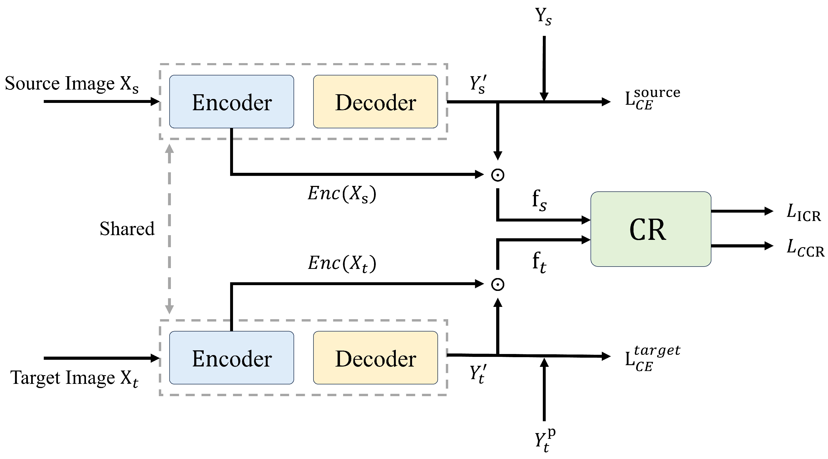
In the context of remote sensing image segmentation, domain adaptation presents unique challenges due to the inherent variability in image characteristics across different domains. The goal is to transfer knowledge from a labeled source domain to an unlabeled target domain with significant discrepancies in noise levels, spatial resolution, and environmental conditions. To address these challenges, we introduce a novel scene covariance alignment (SCA) model. The SCA model facilitates robust feature alignment between source and target domains by leveraging scene-level feature pooling and covariance regularization, thus enabling effective domain adaptation and improved generalization in complex environments.

The core of the SCA model builds on the DeepLabV2 framework with ResNet-50 as its backbone for feature extraction. This model is augmented by two key innovations: the scene feature pooling (SFP) module, which aggregates scene-specific features, and the covariance regularization (CR) mechanism, which reinforces feature alignment across domains. Together, these components ensure the model’s adaptability to domain shifts while preserving scene-level feature integrity. The framework of the SCA model is shown in Figure 1.

2.1. Scene Feature Pooling (SFP)

Remote sensing images exhibit complex spatial and scene characteristics, such as spatial distribution, texture, and spectral features, with unique feature distributions across different scenes. The scene feature pooling (SFP) module captures domain-specific multi-scale scene feature information and integrates it with land-cover class features to generate scene-level centroids for land-cover classes. The SFP module comprises three components: Multi-Scale Feature Pooling Layer, Context Attention Fusion Layer, and Scene-Level Centroid Generation.

The Multi-Scale Feature Pooling Layer applies multiple pooling operations with different window sizes to the feature map $\mathit{F}\in {\mathbb{R}}^{H\times W\times C}$. Each pooling output is dimensionally reduced to a unified channel number $C^{\prime }$ via $1\times 1$ convolution. The features from different scales are resized to the original feature map size $H\times W$ using bilinear interpolation and concatenated along the feature dimension, resulting in a comprehensive feature ${\mathit{F}}_{pool}\in {\mathbb{R}}^{H\times W\times C^{″}}$, where $C^{″}=n·C^{\prime }$, and n is the number of pooling windows.

The Context Attention Fusion Layer captures key features and suppresses redundant information in the feature map through channel attention, spatial attention, and self-attention mechanisms. The outputs of the three mechanisms are denoted as ${\mathit{F}}_c,{\mathit{F}}_s,{\mathit{F}}_a$, respectively, with the formulas as follows:

$${\mathit{F}}_c=\mathit{F}·A_c=\mathit{F}·\sigma \left(\mathrm{FC}\left(\mathrm{ReLU}\left(\mathrm{FC}({\mathit{F}}_{avg}+{\mathit{F}}_{max})\right)\right)\right)$$

(1)

where ${\mathit{F}}_{avg}$ and ${\mathit{F}}_{max}$ represent the spatial average pooling and maximum pooling of the comprehensive feature map, respectively, and $A_c$ is the channel attention weight.

$${\mathit{F}}_s=\mathit{F}·A_s=\mathit{F}·\sigma \left(\mathrm{Conv}2\mathrm{D}\left([{\mathit{F}}_{s\_avg},{\mathit{F}}_{s\_max}]\right)\right)$$

(2)

where ${\mathit{F}}_{s\_avg}$ and ${\mathit{F}}_{s\_max}$ represent the channel-wise average pooling and maximum pooling of the comprehensive feature map, respectively, and $A_s$ is the spatial attention weight.

$${\mathit{F}}_a=\mathrm{Softmax}\left({\mathit{QK}}^T\right)\mathit{V}$$

(3)

where $\mathit{Q},\mathit{K},\mathit{V}$ are the linear transformations of the feature map. The fused scene feature is denoted as ${\mathit{F}}_{context}\in {\mathbb{R}}^{H\times W\times C^{″}}$, obtained by combining ${\mathit{F}}_c,{\mathit{F}}_s,{\mathit{F}}_a$.

Finally, the Context Attention Fusion Layer’s scene features are combined with the coarse prediction output from the network to generate scene-level centroids $\mathit{f}\in {\mathbb{R}}^{N\times C^{″}}$, where N is the number of land-cover classes. The generation formula is as follows:

$$\mathit{f}={\displaystyle \frac{1}{H\times W}}\sum _{k=1}^{H\times W}{\mathit{Y}}_k^{\prime }\odot {\mathit{F}}_{context}$$

(4)

Here, ${\mathit{Y}}^{\prime }\in {\mathbb{R}}^{N\times H\times W}$ represents the coarse prediction from the segmentation network, and ⊙ denotes element-wise multiplication. The Multi-Scale Feature Pooling Layer captures diverse feature distributions of scenes through local-to-global multi-scale pooling. The Context Attention Fusion Layer enhances contextual feature representation by integrating channel attention, spatial attention, and self-attention mechanisms.

2.2. Covariance Regularization for Robust Feature Alignment

To effectively align the category-specific scene features extracted by the scene feature pooling module between the source and target domains, we introduce a covariance regularization (CR) [32,33] mechanism. The core idea of this mechanism is to reduce the distribution discrepancy between the source and target domains by aligning the covariance of features within the same scene and separating the features between different scenes. Specifically, for different samples of the same scene, we want their feature representations to be as similar as possible, meaning the covariance matrix of the features within a scene should be “concentrated”. This ensures that samples of the same scene category have high consistency in the feature space. On the other hand, features from different scenes should be as separated as possible, meaning the covariance matrix between scenes should be “dispersed”. By doing so, we ensure a clear distinction between features of different scenes, thus reducing cross-scene confusion. The core of covariance regularization lies in calculating the correlation between scene features. For two feature vectors ${\mathit{f}}_1$ and ${\mathit{f}}_2$, we use cosine similarity as the measure of their correlation.

$$\mathrm{Corr}({\mathit{f}}_1,{\mathit{f}}_2)={\displaystyle \frac{{({\mathit{f}}_1-{\mu }_{{\mathit{f}}_1})}^T({\mathit{f}}_2-{\mu }_{{\mathit{f}}_2})}{{\parallel {\mathit{f}}_1-{\mu }_{{\mathit{f}}_1}\parallel }_2{\parallel {\mathit{f}}_2-{\mu }_{{\mathit{f}}_2}\parallel }_2}}$$

(5)

where ${\mu }_{f_1}$ and ${\mu }_{f_2}$ represent the mean vectors of ${\mathit{f}}_1$ and ${\mathit{f}}_2$. In this way, the calculated correlation value reflects the angular difference between the two feature vectors. A value closer to 1 indicates higher similarity, while a value closer to −1 indicates greater dissimilarity. To guide feature alignment, we design the loss function for covariance regularization.

$$L_{\mathrm{CR}}({\mathit{f}}_1,{\mathit{f}}_2)=-{\displaystyle \frac{1}{N^2}}\sum _{i=1}^N\sum _{j=1}^{N}log\left(A_{ij}\left(\mathrm{Corr}({\mathit{f}}_1,{\mathit{f}}_2)\right)\right)$$

(6)

where $A_{ij}$ is defined as

$$A_{ij}\mathrm{Corr}({\mathit{f}}_1,{\mathit{f}}_2)=\left\{\begin{array}{cc}\mathrm{Corr}({\mathit{f}}_1,{\mathit{f}}_2)\hfill & \mathrm{if}i=j\hfill \\ max(1-\mathrm{Corr}({\mathit{f}}_1,{\mathit{f}}_2),ϵ)\hfill & \mathrm{if}i\ne j\hfill \end{array}\right.$$

(7)

where $ϵ$ is a small value used to avoid logarithm with zero. This loss function ensures that the elements on the diagonal (i.e., samples from the same scene) have high correlation, while the elements off the diagonal (i.e., samples from different scenes) have low correlation. Therefore, CR helps the model effectively align scene features between the source and target domains, improving the model’s generalization ability in cross-domain tasks.

2.3. Transferability Analysis

The ability of a model to adapt to unseen domains with different characteristics is critical for effective domain adaptation in RSI segmentation. We analyze the transferability of the SCA model under varying conditions, including noise, resolution, scene complexity, and environmental factors such as cloud cover and contrast variations.

2.3.1. Noise Robustness

In real-world scenarios, remote sensing images are often degraded by noise, which can affect model performance. To assess the noise robustness of our model, we introduce a noise parameter $\sigma$ and model the noisy image ${\mathit{X}}_{\mathrm{noisy}}$ as

$${\mathit{X}}_{\mathrm{noisy}}=\mathit{X}+\mathcal{N}(0,{\sigma }^2)$$

(8)

where $\mathcal{N}(0,{\sigma }^2)$ represents Gaussian noise with zero mean and variance ${\sigma }^2$. Covariance regularization helps preserve feature consistency by minimizing the expected difference between the original and noisy features:

$$\mathbb{E}[\parallel f\left(X\right)-f\left({\mathit{X}}_{\mathrm{noisy}}\right){\parallel }_2^2]\le K{\sigma }^2$$

(9)

Here, K is a constant dependent on the model architecture. This ensures that the SCA model can maintain stable feature representations even in the presence of significant noise.

2.3.2. Resolution Invariance

Remote sensing images are often captured at varying resolutions depending on sensor specifications or acquisition conditions. The SCA model addresses this challenge by employing a multi-scale feature extraction strategy, allowing it to generalize across different resolutions. For a given input image $\mathit{X}$, we generate scaled versions ${\left\{{\mathit{X}}_s\right\}}_{s=1}^S$, where s represents the scale factor. The final feature representation is computed as

$$f_{\mathrm{multi}}\left(\mathit{X}\right)={\displaystyle \frac{1}{S}}\sum _{s=1}^{S}f\left({\mathit{X}}_s\right)$$

(10)

Covariance regularization ensures alignment of features across different scales:

$$L_{\mathrm{scale}}=\sum _{s_1\ne s_2}{L}_{\mathrm{CR}}(f\left({\mathit{X}}_{s_1}\right),f\left({\mathit{X}}_{s_2}\right))$$

(11)

This multi-scale alignment enables the model to adapt to varying resolutions, a key requirement in real-world remote sensing applications.

2.3.3. Scene Complexity Adaptation

Scene complexity in remote sensing images can vary significantly, from simple landscapes to highly heterogeneous environments. To handle these variations, we introduce a scene complexity measure $\mathcal{C}\left(\mathit{X}\right)$ based on the entropy of local image patches:

$$\mathcal{C}\left(\mathit{X}\right)=-\sum _{p\in \mathcal{P}}\sum _i{p}_{i}log{p}_i$$

(12)

where $\mathcal{P}$ represents the set of local patches in the image, and $p_i$ is the normalized intensity histogram for each patch. The feature extraction process adapts to the scene complexity measure as follows:

$$f_{\mathrm{adapted}}\left(\mathit{X}\right)=f\left(\mathit{X}\right)+\alpha \mathcal{C}\left(\mathit{X}\right)·g\left(\mathit{X}\right)$$

(13)

where $g\left(\mathit{X}\right)$ is an additional set of features designed to capture fine-grained details, and $\alpha$ is a learnable parameter. This mechanism allows the model to adjust dynamically to different levels of scene complexity, improving segmentation performance in complex environments.

2.3.4. Cloud Cover Compensation

Cloud cover poses a significant challenge in remote sensing, often obscuring important details in the imagery. To address this, we introduce a cloud detection module $D\left(\mathit{X}\right)$ that generates a cloud probability map. The feature extraction process is then modified as

$$f_{\mathrm{cloud}}\left(\mathit{X}\right)=(1-D\left(\mathit{X}\right))\odot f\left(\mathit{X}\right)+D\left(\mathit{X}\right)\odot h\left(\mathit{X}\right)$$

(14)

where $h\left(\mathit{X}\right)$ represents cloud-specific features. Covariance regularization ensures smooth transitions between clear and cloudy regions, allowing the model to handle cloud interference effectively.

2.3.5. Contrast Normalization

Variation in image contrast is another challenge in remote sensing. To mitigate this, we apply a local contrast normalization (LCN) layer prior to feature extraction:

$${\mathit{X}}_{\mathrm{LCN}}={\displaystyle \frac{\mathit{X}-{\mu }_{\mathrm{local}}}{\sqrt{{\sigma }_{\mathrm{local}}^2+ϵ}}}$$

(15)

where ${\mu }_{\mathrm{local}}$ and ${\sigma }_{\mathrm{local}}$ represent the local mean and standard deviation computed over small image patches. This step ensures that the model is less sensitive to global contrast variations, improving the robustness of the feature extraction process.

2.4. Training Procedure

The SCA model is trained using a stage-wise strategy designed to mitigate error propagation when generating pseudo-labels in the target domain. The total loss function is defined as

$$L=L_{\mathrm{CE}}^{\mathrm{source}}+{\lambda }_1{L}_{\mathrm{CE}}^{\mathrm{target}}+{\lambda }_2{L}_{\mathrm{ICR}}+{\lambda }_3(L_{\mathrm{CCR}}+L_{\mathrm{scale}})+{\lambda }_4{L}_{\mathrm{adapt}}$$

(16)

Here, $L_{\mathrm{CE}}^{\mathrm{source}}$ and $L_{\mathrm{CE}}^{\mathrm{target}}$ represent the cross-entropy losses for the source and target domains, respectively. $L_{\mathrm{ICR}}$ and $L_{\mathrm{CCR}}$ denote the intra-domain and cross-domain covariance regularization losses. $L_{\mathrm{scale}}$ enforces scale invariance, and $L_{\mathrm{adapt}}$ accounts for scene complexity, cloud cover, and contrast normalization components. The hyperparameters ${\lambda }_i$ control the relative contribution of each term with their sum equal to 4.

Optimization is carried out using stochastic gradient descent (SGD) with momentum. The parameter update rule is

$${\theta }_{t+1}={\theta }_t-\eta (\nabla L\left({\theta }_t\right)+m({\theta }_t-{\theta }_{t-1}))$$

(17)

where $\eta$ represents the learning rate, m is the momentum coefficient, and ${\theta }_t$ denotes the model parameters at iteration t. A polynomial learning rate decay schedule is used to ensure stable convergence:

$${\eta }_t={\eta }_0{\left(1-{\displaystyle \frac{t}{T}}\right)}^p$$

(18)

where ${\eta }_0$ is the initial learning rate, T represents the total number of iterations, and p denotes the decay power. This comprehensive training procedure, combined with the novel architectural innovations, allows the SCA model to achieve robust performance across a wide range of remote sensing tasks and domains.

3. Experiments and Results

In this section, we evaluate the effectiveness of the proposed scene covariance alignment (SCA)model for domain adaptation in remote sensing image (RSI) segmentation. Our experiments are designed to test the model’s ability to generalize across different domains with substantial variability in spatial resolution, noise levels, and environmental conditions. We compare our model against several state-of-the-art baselines and perform ablation studies to assess the contribution of each key component, including the scene feature pooling (SFP) module and covariance regularization (CR) mechanism. Furthermore, we analyze the model’s robustness to contrast, noise, resolution changes, and scene complexity.

3.1. Datasets

We evaluated the scene covariance alignment (SCA) model using two remote sensing datasets that present significant domain adaptation challenges due to differences in geographic location, sensor characteristics, and environmental conditions.

The LoveDA (A Remote Sensing Land-Cover Dataset for Domain Adaptive Semantic Segmentation. Retrieved from https://github.com/Junjue-Wang/LoveDA, accessed on 10 September 2024) dataset [34] is a large-scale land cover classification dataset, consisting of 5987 high-resolution remote sensing images (1024 × 1024 pixels, 0.3 m/pixel) from three Chinese cities: Nanjing, Changzhou, and Wuhan. The images provide three channels: Red, Green, and Blue (RGB), and cover seven land cover categories: Background, Building, Road, Water, Bare Land, Forest, and Agriculture. The dataset is divided into urban and rural scenes. The rural scene contains 2358 images, with 1366 used for training and 992 for testing. The urban scene contains 1833 images, with 1156 used for training and 677 for testing. The LoveDA dataset covers approximately 3000 square kilometers of land and exhibits rich intra-class and inter-class diversity.

The Yanqing dataset contains more than 500 high-resolution remote sensing images (2048 × 2048 pixels, 0.5 m/pixel) captured by the GaoJing-1 satellite over the Yanqing area in Beijing, China, covering an area of approximately 260 square kilometers. The images also provide three channels: Red, Green, and Blue, with radiometric calibration and atmospheric correction performed using the Fast Line-of-sight Atmospheric Analysis of Spectral Hypercubes (FLASH) algorithm [35]. A machine learning-based cloud detection algorithm is used to identify and mask cloud-covered areas. As our target domain, the Yanqing dataset presents unique geographical and environmental features compared to the LoveDA dataset, posing distinct challenges for domain adaptation.

For ground truth data, a team of remote sensing experts manually annotated 100 images from the Yanqing dataset for seven land cover classes consistent with the LoveDA dataset. We employed a rigorous cross-validation process, with each image independently annotated by two experts. Discrepancies were resolved through consensus discussions. To evaluate the model’s performance on the target domain, we randomly selected 20% of the annotated images as a held-out validation set.

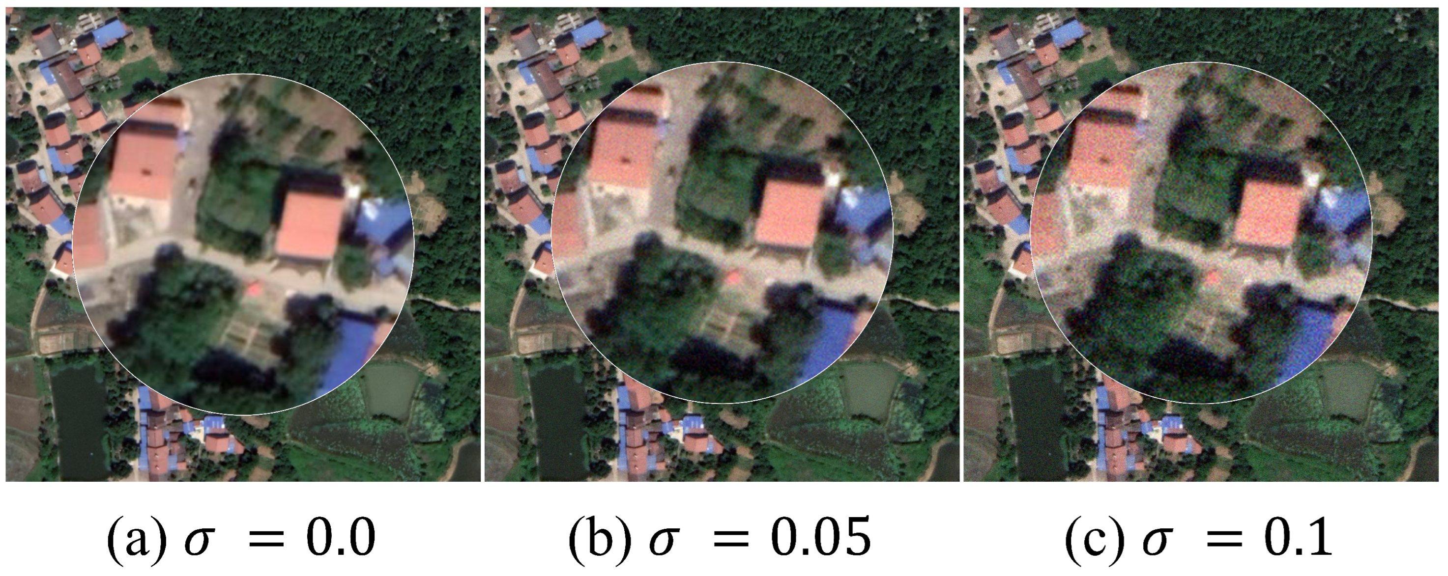
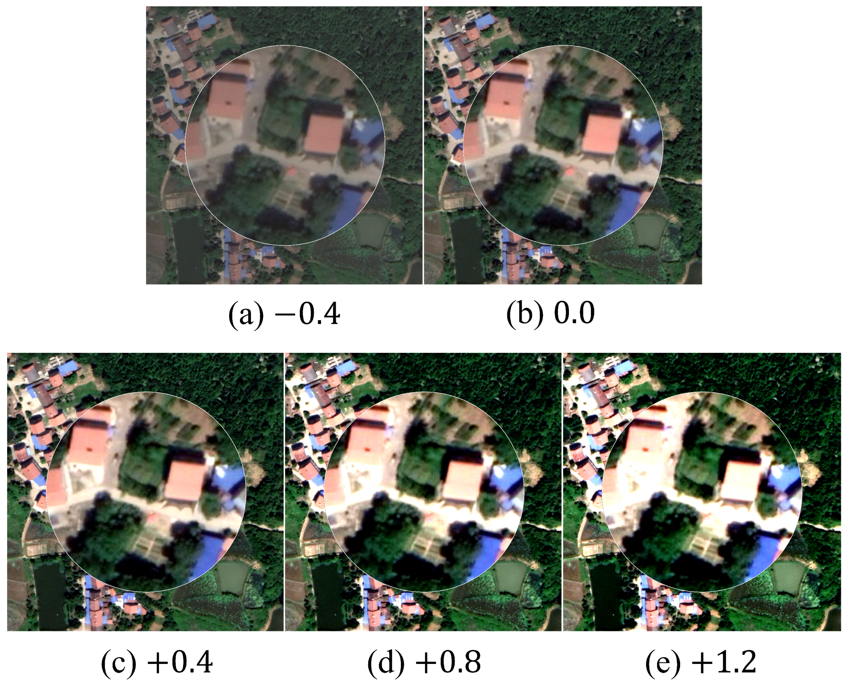
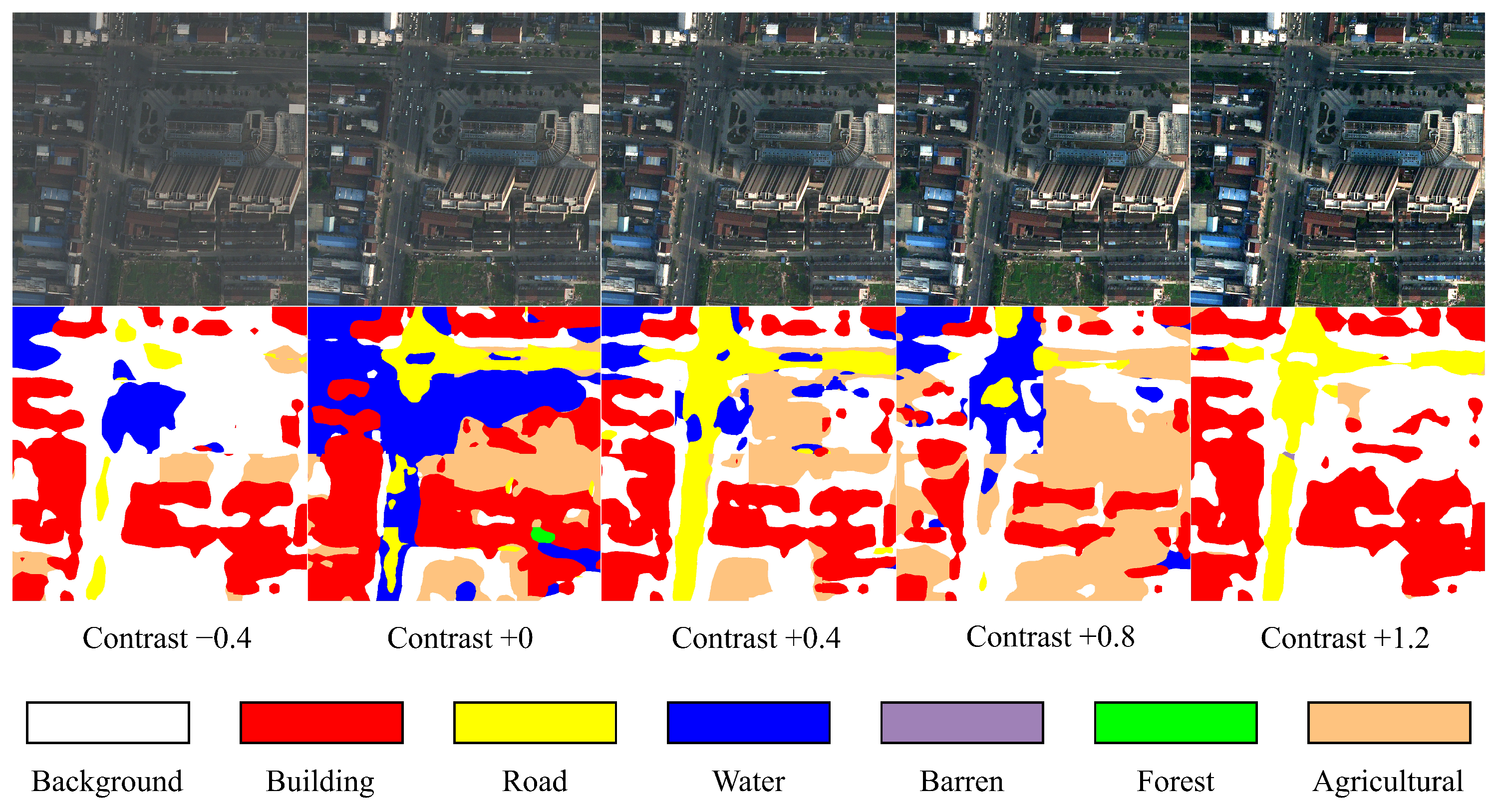
To assess the SCA model’s robustness and transferability, we systematically augmented the LoveDA dataset and Yanqing dataset. We introduced two levels of Gaussian noise ($\sigma$ = 0.05, 0.1) to simulate sensor noise and atmospheric interference (Figure 2). 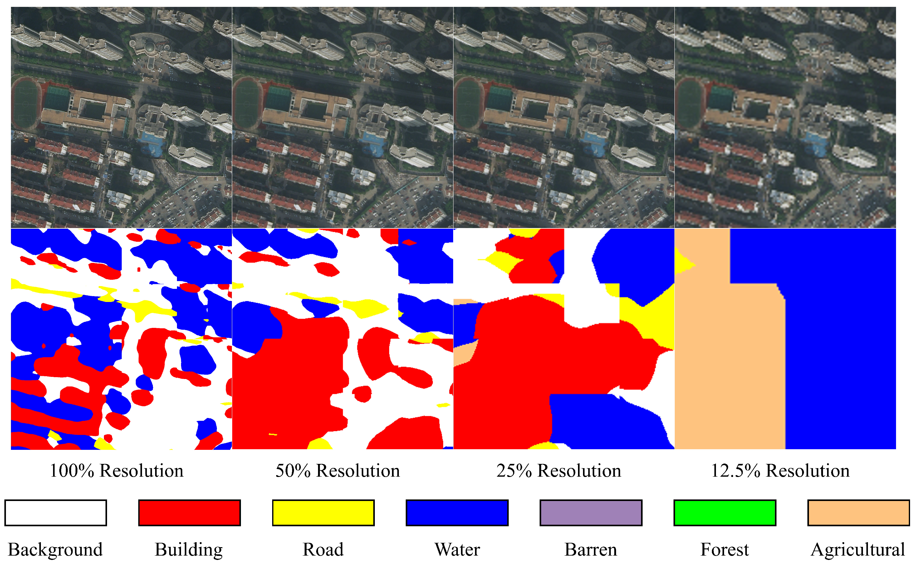Image contrast was altered using linear contrast stretching with values of −0.4, 0.4, 0.8, and 1.2 to mimic variations in illumination conditions (Figure 3). Furthermore, we generate 3/4, 1/2, and 1/4 resolution versions of the images using bilinear interpolation to evaluate the model’s performance at different spatial resolutions.

3.2. Experimental Settings

Experimental Environment.All models are implemented using the PyTorch framework, and all experiments are conducted in a Linux environment using an NVIDIA GeForce RTX 4090 24GB GPU.

Network Architecture and Training. The core of the SCA model builds on the DeepLabV2 framework with ResNet-50 as its backbone for feature extraction. All original images are cropped into 512 × 512 patches as input to the model, with three channels: R, G, and B. In the scene feature pooling module, the input data are a feature map of size 2048 × 32 × 32. It is then processed through pooling windows with sizes 1 × 1, 2 × 2, 3 × 3, and 6 × 6, followed by bilinear interpolation and feature fusion to obtain a consolidated feature map. During the training, we used the Stochastic Gradient Descent (SGD) optimizer with a momentum of 0.9 and a weight decay of 0.0005. The learning rate was initially set to 0.01, and a poly schedule with power 0.9 was applied. And The hyperparameters ${\lambda }_1$, ${\lambda }_2$, ${\lambda }_3$, ${\lambda }_4$ in the loss function are set to 0.8, 0.8, 0.8, and 1.6. In addition, we employ a staged process to train the model, preventing the accumulation of error-prone pseudo-labels generated during self-training. The maximum number of stages and iterations are set to 5 and 1000.

3.3. Evaluation Metrics

To rigorously assess the performance of the scene covariance alignment (SCA) model, we employed a comprehensive set of evaluation metrics. These metrics provide a multifaceted view of the model’s segmentation accuracy and its ability to generalize across diverse remote sensing scenes.

The primary metric used is the Mean Intersection over Union (mIoU), which quantifies the average overlap between the predicted segmentation and the ground truth across all categories. For a given class i, the IoU is calculated as

$${\mathrm{IoU}}_i={\displaystyle \frac{|{\mathrm{TP}}_i|}{|{\mathrm{TP}}_i|+|{\mathrm{FP}}_i|+|{\mathrm{FN}}_i|}}$$

(19)

where ${\mathrm{TP}}_i$, ${\mathrm{FP}}_i$, and ${\mathrm{FN}}_i$ represent the true positive, false positive, and false negative pixels for class i, respectively. The mIoU is then computed as the average IoU across all N classes:

$$\mathrm{mIoU}={\displaystyle \frac{1}{N}}\sum _{i=1}^N{\mathrm{IoU}}_i$$

(20)

To complement the mIoU, we also report the Pixel Accuracy (PA), which provides a global measure of correctly classified pixels across the entire image. PA is defined as

$$\mathrm{PA}={\displaystyle \frac{{\sum }_{i=1}^N{\mathrm{TP}}_i}{{\sum }_{i=1}^N({\mathrm{TP}}_i+{\mathrm{FP}}_i)}}$$

(21)

3.4. Baseline Methods

To evaluate the effectiveness of the scene covariance alignment (SCA) model, we conducted comparisons against four baseline methods, each representing a distinct approach to domain adaptation in remote sensing image segmentation. The first baseline is DeepLabV2 [36] with a ResNet-50 [37] backbone, a powerful semantic segmentation model without specific domain adaptation techniques. We also compare against the Domain-Adversarial Neural Network (DANN) [38], which employs adversarial learning to align feature distributions of source and target domains. The third is AdaptSegNet [39], which extends adversarial domain adaptation specifically to segmentation tasks by applying adversarial learning in the output space. The fourth is De-GLGAN [31], which designs an adaptive method based on high-low frequency decomposition and builds a global-local adversarial learning model based on this method. Finally, MemoryAdaptSegNet [40] incorporates an invariant feature memory module within adversarial learning to preserve domain-level information, overcoming the issue of insufficient pseudo-invariant features. These baselines provide a comprehensive framework for assessing the SCA model’s performance across diverse geographical and environmental conditions in remote sensing imagery.

3.5. Quantitative Results

Table 1. Performance comparison between baseline models and the SCA model for the LoveDA → Yanqing District domain adaptation task.

Method	LoveDA → Yanqing (mIoU)	LoveDA → Yanqing (PA)
DeepLabV2 (ResNet-50)	48.3	73.1
DANN	54.2	76.4
AdaptSegNet	57.6	78.9
De-GLGAN	60.3	80.7
MemoryAdaptSegNet	62.9	80.1
SCA (Ours)	63.1	82.5

shows the performance comparison of the SCA model against the baselines for the domain adaptation tasks from LoveDA to Yanqing District.

The results demonstrate that the SCA model significantly outperforms baseline models in the domain adaptation task from LoveDA to Yanqing District. The SCA model achieves a 5.5% improvement in mIoU compared to AdaptSegNet, indicating its superior generalization capabilities across different geographic and environmental conditions.

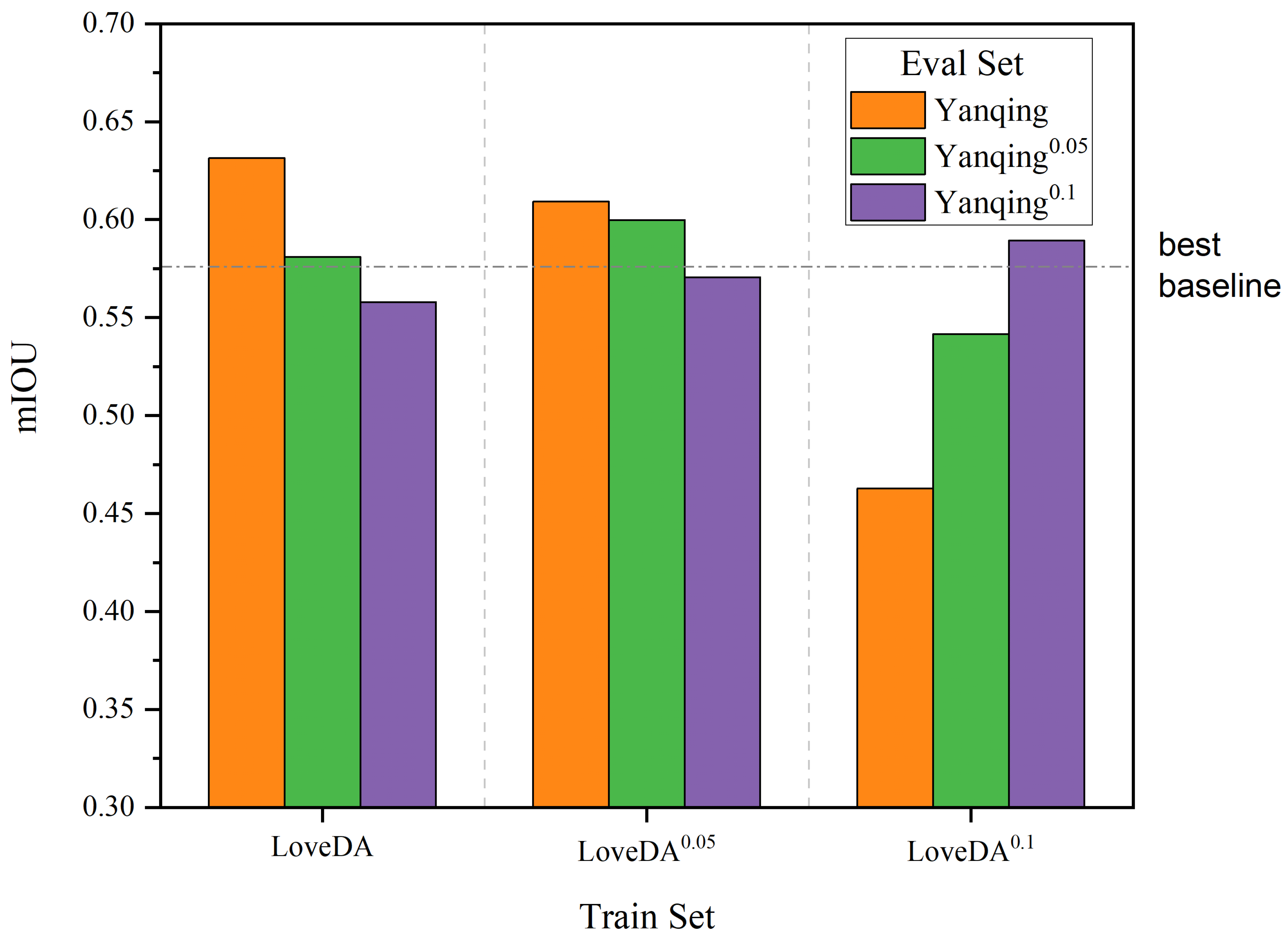
3.6. Robustness to Contrast, Noise and Resolution Variations

As shown in Figure 4 and Figure 5, compared to the best baseline model (AdaptSegNet), the SCA model demonstrates better robustness to contrast and noise. It maintains higher mIoU scores in most cases, even under severe contrast changes and significant noise level differences.

We also tested the model’s robustness to resolution changes by downsampling the target domain images.

Table 2. mIoU results under different downsampling factors for the LoveDA → Yanqing District task.

Downsampling Factor	DeepLabV2	DANN	AdaptSegNet	SCA (Ours)
1× (Original)	48.3	54.2	57.6	63.1
0.75×	45.2	51.0	54.5	60.3
0.5×	41.8	47.5	50.6	56.4
0.25×	37.9	42.8	45.2	51.9

shows the mIoU results under different downsampling factors for the LoveDA to Yanqing District task.

The SCA model consistently outperforms the baselines across all downsampling factors, demonstrating its robustness to resolution changes, which is particularly relevant for handling remote sensing data from different sensors or acquisition conditions.

3.7. Ablation Studies

To demonstrate and quantify the contributions of each component within the SCA model to the unsupervised domain adaptation semantic segmentation task on remote sensing images, we conducted ablation studies. In three separate ablation experiments, we respectively removed the scene feature pooling module, the covariance regularization mechanism, and the multi-scale feature pooling operations from the SCA model.

Table 3. Ablation study results for the LoveDA → Yanqing District task.

Method	mIoU	PA
SCA (Full Model)	63.1	82.5
Without SFP	57.3	77.6
Without Covariance Regularization (CR)	58.5	79.2
Without Multi-Scale Features	59.0	80.1

presents the results of the ablation studies for the LoveDA to Yanqing District task.

The ablation study results show that the scene feature pooling module, the covariance regularization mechanism, and the multi-scale feature pooling operations play indispensable roles in the model. Removing these components significantly degrades the model’s performance. In particular, the scene feature pooling module is crucial for enabling the SCA model to adapt to complex and dynamic scene-level features.

In addition, we conducted experiments on the selection of loss function hyperparameters ${\lambda }_i$.

Table 4. mIoU results under different loss function hyperparameters ${\lambda }_i$ for the LoveDA → Yanqing District task.

Lambda1	Lambda2	Lambda3	Lambda4	mIoU
1.0	1.0	1.0	1.0	62.2
1.5	0.8	0.8	0.9	62.1
2.0	0.6	0.6	0.8	60.3
0.8	1.5	0.8	0.9	61.3
0.6	2.0	0.6	0.8	58.6
0.8	0.8	1.5	0.9	61.0
0.6	0.6	2.0	0.8	62.9
0.8	0.8	0.8	1.6	63.1
0.6	0.6	1.0	2.0	62.8

presents the results of this experiment for the LoveDA to Yanqing District task. We observed that increasing the weight of the target domain prediction loss or the intra-domain covariance alignment loss, while reducing the weights of other losses, resulted in a decrease in the final segmentation mIoU compared to using equal weights. In contrast, increasing the weight of the cross-domain covariance alignment loss, multi-scale loss, and complex scene loss led to an improvement in the final segmentation mIoU. As show in Table 4, the best results were achieved when ${\lambda }_1=0.8$, ${\lambda }_2=0.8$, ${\lambda }_3=0.8$ and ${\lambda }_4=1.6$. We suggest that the weight of these two types of losses can be appropriately increased. This indicates that multi-scale feature pooling and covariance regularization mechanisms play an indispensable role in the model.

3.8. Qualitative Results

Figure 6 provides a visual comparison of the segmentation performance of the SCA model at different contrast levels. The SCA model demonstrates strong generalization capabilities, with the semantic segmentation results gradually improving as the contrast increases from −0.4 to +0.8, featuring clearer category boundaries and richer details. However, over-segmentation occurs when the contrast reaches +1.2.

Figure 7 highlights the model’s performance across different image resolutions. The SCA model consistently produces clearer and more accurate segmentations at all resolution levels. However, due to the massive amount of object detail in urban images, it also experiences significant degradation at ultra-low resolutions.

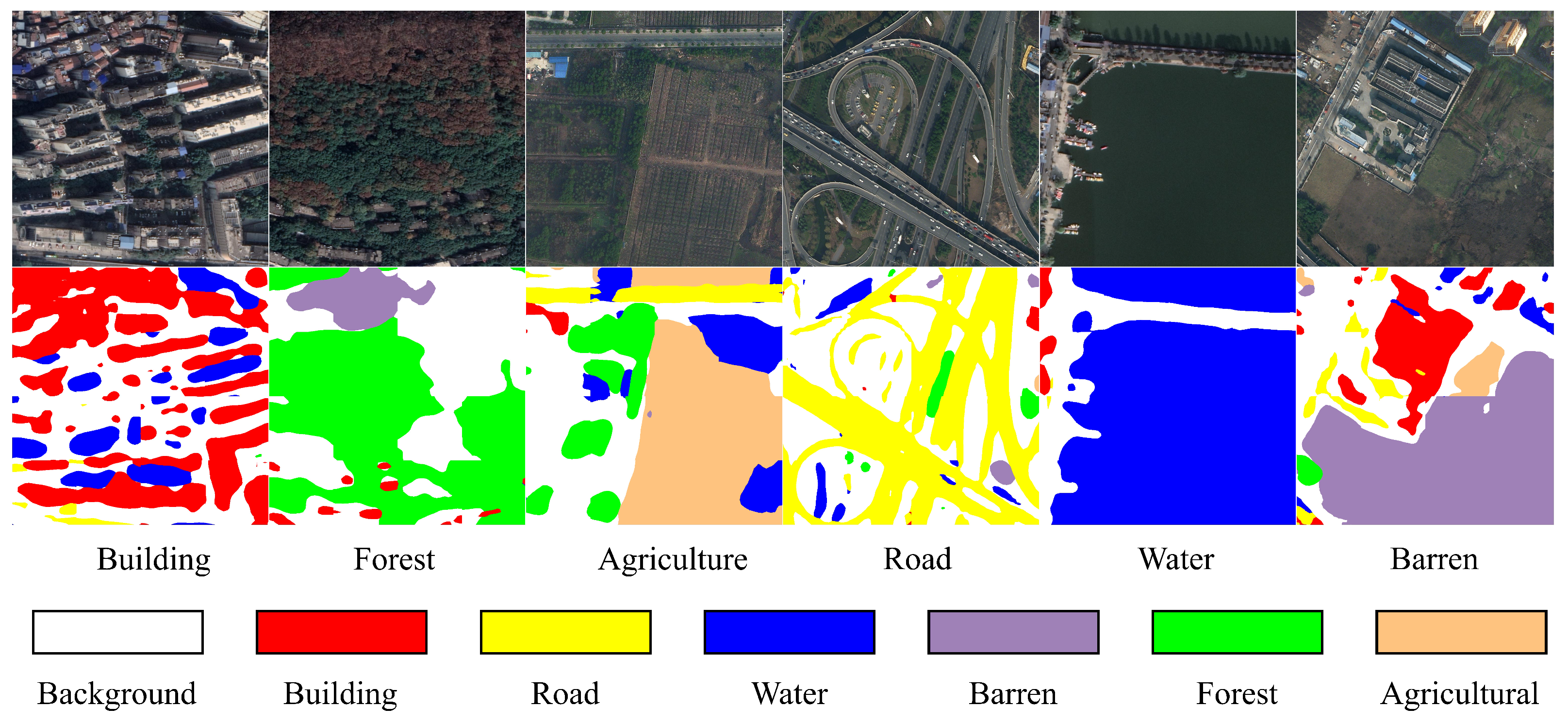
Figure 8 illustrates the segmentation results across different scenarios, including complex urban and rural environments. The SCA model exhibits more spatially coherent segmentations, particularly in heterogeneous landscapes.

These visual results strongly support the quantitative findings, further demonstrating the SCA model’s ability to produce accurate and robust segmentations across a wide range of challenging scenes, including low contrast, varying resolutions, and complex scene structures.

The experimental results presented in this work demonstrate the effectiveness of the SCA model in addressing the challenges of domain adaptation in remote sensing image (RSI) segmentation. The SCA model outperforms state-of-the-art baseline models in most cases, showcasing its ability to generalize across diverse target domains with varying noise levels, spatial resolutions, and environmental conditions.

3.9. Model Inference

Inference time, as part of model performance, is a critical consideration for actual deployment. Using an NVIDIA (Santa Clara, CA, USA) GeForce RTX 4090 24G and PyTorch 1.10, we conducted multiple inference tests on the LoveDA and Yanqing datasets. The results show that it takes an average of 0.489 s to infer a single 1024 × 1024 RGB remote sensing image. Additionally, we conducted the same inference tests on a 12 vCPU Intel(R) (Santa Clara, CA, USA) Xeon(R) Platinum 8352V CPU@2.10 GHz, which yielded an average inference time of 25.245 s.

The requirements for inference time in real-time applications depend on the specific definition of real-time and the application scenario. For tasks with non-continuous input, such as user-triggered analyses, this inference time is acceptable. However, for real-time video stream processing, this inference time is clearly inadequate.

4. Discussion

In this section, we discuss the key contributions of the SCA model and the broader implications of our findings while also exploring potential areas for future research.

4.1. Effectiveness of Scene-Level Feature Alignment

A central contribution of the SCA model is the introduction of scene-level feature alignment of ground object categories through the scene feature pooling (SFP) module and covariance regularization (CR) mechanism. The results from our ablation studies clearly indicate that both components are essential for achieving robust performance across different domains. By pooling scene-specific features and aligning their covariance across domains, the model ensures that critical scene-level characteristics are consistently captured, even in the presence of domain shifts. This is particularly important in remote sensing applications where geographic diversity and environmental variability can result in significant differences between source and target domains.

Compared to existing adversarial or self-training methods (which typically do not consider the feature variations of ground object categories across different scenes), which often focus on aligning global feature distributions, the SCA model goes a step further by explicitly targeting scene-level features. This finer granularity in feature alignment ensures that the model can handle complex and heterogeneous environments more effectively, as evidenced by the model’s superior performance on both the LoveDA Rural to Urban and LoveDA Rural to Yanqing tasks.

4.2. Robustness to Contrast, Noise and Resolution Changes

The SCA model exhibits significant robustness to contrast and noise, as demonstrated by our experiments applying contrast and noise to both source and target domains. Covariance regularization plays a crucial role in this robustness, maintaining feature consistency even in environments with high contrast differences and high noise levels. This is particularly important for real-world remote sensing applications, where images are often affected by sensor noise, atmospheric interference, environmental lighting, or adverse weather conditions. The model’s ability to maintain high segmentation accuracy under such conditions makes it a strong candidate for practical deployment in challenging operational environments.

Similarly, the SCA model adopts a multi-scale feature extraction strategy to ensure robustness against resolution changes. This approach enables the model to learn scene features across multiple scales—from local to global—effectively adapting to common spatial resolution variations encountered in real-world applications. This is particularly important when dealing with remote sensing data from different sensors or platforms, as it reduces the amount of preprocessing required and mitigates the associated loss of information.

4.3. Handling Scene Complexity and Environmental Variability

The complexity of remote sensing images, particularly in terms of category distribution differences and category feature distribution differences, poses significant challenges for segmentation models. The SCA model addresses this by incorporating a scene complexity measure, which allows the model to adapt its feature extraction process dynamically based on local scene characteristics. This adaptive mechanism is crucial for improving segmentation performance in scenes with varying levels of complexity, such as densely built urban areas or heterogeneous agricultural landscapes.

4.4. Implications for Remote Sensing Applications

The strong performance of the SCA model across multiple domain adaptation tasks has significant implications for a wide range of remote sensing applications, including land-use classification, urban planning, disaster management, and environmental monitoring. The ability to generalize across domains with minimal labeled data from the target domain reduces the reliance on extensive and costly ground truth labeling efforts, making it more feasible to deploy remote sensing segmentation models in new geographic regions or under changing environmental conditions.

Furthermore, the model’s robustness to noise, resolution variations, and environmental factors such as contrast and scene complexity enhances its practicality in real-world scenarios. Remote sensing applications often involve data from various sensors, acquired under different conditions, and the SCA model’s ability to adapt to these variations ensures that it can be applied in diverse operational contexts without significant performance degradation.

4.5. Under Low-Light and Noisy Conditions

In practical applications of remote sensing image segmentation, remote sensing images are often affected by various factors, such as insufficient illumination, sensor noise, weather conditions, and the blurriness of target objects. In particular, remote sensing images captured in low-light environments suffer from reduced contrast and color saturation, along with increased sensor noise, leading to a significant decrease in the distinguishability and resolution of ground object features. Additionally, texture and boundary information may be overwhelmed by noise.

Under such conditions, the performance of the SCA model may decline. However, the multi-scale feature extraction and covariance regularization mechanisms employed by the model still offer certain advantages. Multi-scale feature extraction can identify useful information at different scales. Smaller pooling windows help capture local texture and boundary features, even when these features are disrupted by noise, while larger scales emphasize more stable global scene structural information. By fusing information across multi-scale feature spaces, the model can still extract a degree of discriminative features under low-light and high-noise conditions.

To mitigate the effects of low-light and high-noise conditions on the imagery, image enhancement structures [41,42,43] (e.g., denoising, deblurring, and contrast enhancement) can be incorporated before the model’s encoder. This improves the quality of the input data, enabling the SCA model to better align features and perform segmentation effectively.

4.6. Limitations and Future Work

While the SCA model achieves strong results, there are several areas that warrant further investigation. First, although the model handles scene complexity effectively, its performance could be further improved by integrating additional weather or atmospheric correction modules. This would allow the model to better handle extreme environmental conditions, such as heavy fog, snow, or seasonal vegetation changes.

Another limitation lies in the reliance on pseudo-labeling during unsupervised domain adaptation. While this technique helps improve performance on the target domain, errors in pseudo-label generation can propagate through the model and impact overall accuracy. Future work could explore more robust pseudo-labeling strategies or semi-supervised learning techniques to mitigate these errors.

Lastly, while the model has been tested on aerial and satellite imagery, its applicability to other forms of remote sensing data, such as hyperspectral or radar imagery, remains to be explored. Adapting the SCA model to these modalities could open new avenues for domain adaptation in even more challenging remote sensing applications.

5. Conclusions

The scene covariance alignment (SCA) model introduces a transformative approach to domain adaptation in remote sensing by emphasizing scene-level feature alignment. Central to its innovation are the scene feature pooling (SFP) module and covariance regularization (CR) mechanism, which collaboratively ensure robust performance across domains by aligning critical scene-level characteristics. This approach addresses challenges inherent in remote sensing, such as geographic diversity and environmental variability, and outperforms traditional adversarial and self-training methods that focus on global feature alignment.

This strong adaptability has profound implications for practical applications in remote sensing, such as land-use classification, urban planning, disaster management, and environmental monitoring. The SCA model’s ability to generalize across domains with minimal labeled target data reduces the reliance on costly ground-truth annotations, enabling deployment in new geographic regions or under varying environmental conditions. Its robustness to operational challenges makes it a promising tool for real-world remote sensing tasks, where data variability is inevitable.

While the SCA model sets a new benchmark in domain adaptation, areas for further improvement remain. Integrating weather and atmospheric correction modules could enhance performance under extreme conditions, such as heavy fog or seasonal vegetation changes. Additionally, refining pseudo-labeling techniques or exploring semi-supervised approaches could mitigate label noise and further enhance target domain performance. Expanding the model’s applicability to other remote sensing modalities, such as hyperspectral or radar imagery, presents another promising direction, potentially extending its impact to a broader range of challenging remote sensing applications.

In summary, the SCA model represents a significant step forward in robust and scalable remote sensing segmentation. Its innovative design not only addresses the complexity of scene-level feature variations but also establishes a framework for future research in domain adaptation, paving the way for broader, more effective deployment of remote sensing technologies.