Check-In Heterogeneous Hypergraph and Personalized Preference Transfers for Cross-City POI Recommendation Method

Abstract

The objective of cross-city recommendation is to suggest points-of-interest (POI) in the target city that may be of interest to users, based on their check-in records from their source city. Although significant progress has been made in studying user preference transfers, there is a lack of research focusing on personalized user preference transfers. Furthermore, the mining of user preferences from the source city is impacted by errors and missing information. To address these challenges, this paper proposes a Check-In Heterogeneous Hypergraph and Personalized Preference Transfers for Cross-City POI Recommendation Method (CHHPPT). Firstly, a check-in heterogeneous hypergraph network is introduced in the user source city preference-mining module. This network, through Heterogeneous Hypergraph Embeddings (HHE), captures user preferences in the source city, thereby mitigating the impact of errors and missing information on user preference. Subsequently, in the user-personalized preference transfer module, a user’s transferable features are obtained through a POI aggregation network. These features are then combined with a meta-network and transfer networks to achieve user-personalized preference transfer. Finally, in the target city point-of-interest recommendation module, a POI-geographical graph is constructed using the geographical information of POI. This graph, in conjunction with category information, yields a joint embedding representation. The final recommendation is achieved by integrating the user-personalized preference transfer embeddings with the target city’s POI embeddings. Extensive experiments conducted on two real-world datasets demonstrate the effectiveness of CHHPPT in cross-city recommendation tasks.

1. Introduction

As urban mobility increases, people are traveling or migrating between cities more frequently. Cross-city recommendations can help users find places that match their interests in different urban environments, whether for business trips or tourism.

Traditional POI recommendation methods are suited for recommending POI within a single city. However, when users are in a new city, traditional algorithms may struggle to provide effective cross-city recommendations, leading to a decline in recommendation quality. The following issues arise in cross-city POI recommendations: (1) User preferences from their home city (source city) cannot be directly transferred to preferences for a new city (target city), due to differences between preferences in the source and target cities (i.e., preference shift); (2) Due to the sparsity of interaction data (whether from source or target city check-ins) and the diversity of candidate POI, semantic information—such as categories, types, ratings, and other details—plays a critical role in shaping user preferences. Furthermore, errors and missing data in the process of extracting user preferences from the source city further complicate the recommendation process.

Existing research has addressed this issue by introducing various approaches. For instance, the study in [1] proposed a probabilistic generative model, Spatio-Temporal Latent Dirichlet Allocation (ST-LDA), to learn region-specific user preferences and group preferences to accommodate changes in user preference. Another study [2] introduced the Location-Sentiment-Aware Recommender System (LSARS), a probabilistic generative model that simulates users’ check-in activities in target cities by adapting to preference transfer and crowd sentiments. Additionally, the study in [3] presented Travel-Intention-Aware Out-of-Town Recommendation (TRAINOR), a cross-city POI recommendation model that utilizes a multi-layer perceptron (MLP) forthe non-linear mapping of preference transfer. However, these methods rely on a common transfer channel for user preferences, which may not be ideal, as each user’s source city preferences vary, necessitating individualized transfer channels.

In addition, there are some studies that explore users’ source city preferences. For example, reference [3] constructs a user check-in graph by utilizing users’ source city check-ins to mine their source city preferences. Reference [4] builds an embedding layer to obtain embedding vectors for users’ source city check-ins, and then uses an attention network to acquire users’ source city preferences. However, these models only retain users’ source city check-ins or treat all of the users’ check-in records as source city check-ins when processing user check-in data. This results in information loss and the introduction of erroneous data, which prevents accurate mining of users’ source city preferences. For example, as shown in the example in Figure 1, the tourist Tom has historical check-ins in his hometown city A as well as in out-of-town cities B and C. It can be easily observed that this user prefers to visit museums and theaters in his hometown city. Before traveling to city C, Tom also left a check-in in city B. Tom’s check-in in city C is not only influenced by his preferences in the hometown city A but is also affected by his check-in preferences in city B. Furthermore, Tom’s check-in preferences in city C have shifted compared to those in his residential city A.

To address the aforementioned issues, this paper proposes the Check-In Heterogeneous Hypergraph and Personalized Preference Transfers for Cross-City POI Recommendation Method (CHHPPT). Unlike previous studies, this paper focuses on cross-city recommendations by constructing a check-in heterogeneous hypergraph to uncover users’ source city preferences. Additionally, personalized preference transfer is achieved through the introduction of POI aggregation networks, meta-networks, and transfer networks. The primary contributions of this work are as follows:

• In the check-in heterogeneous hypergraphs preference-mining module, a user check-in heterogeneous hypergraph is constructed, comprising four types of nodes: users, points of interest (POI), cities, and POI categories. This approach retains missing information in the source city preference mining while avoiding the influence of erroneous information on user preferences. User source city preferences are obtained through Heterogeneous Hypergraph Embedding (HHE).
• In the personalized preference transfer module, a POI-category graph is constructed, and POI embeddings are obtained using the skip-gram. A user’s transferable features are derived through a POI aggregation network. A meta-network is then constructed to learn the weight parameters of the transfer network. Ultimately, the transfer network facilitates the personalized transfer of user preferences.
• In the target city POI recommendation module, a POI-geographical graph is constructed using the geographical information of the POI. This graph, combined with POI category information, is processed through a Graph Convolutional Network (GCN) to obtain a joint embedding representation. The final recommendation is achieved by merging the user-personalized preference transfer embeddings with the target city’s POI embeddings.
• Extensive experiments have validated the effectiveness of the proposed method in enhancing recommendation accuracy.

2. Related Work

2.1. Cross-City POI Recommendation

Cross-city POI recommendation primarily addresses several key challenges, including data sparsity [5,6,7,8], user preference transfer [2,3,4,9,10,11,12], and cold start [13], among others. To address the issue of data sparsity, some studies have used adaptive attention mechanisms to integrate users’ long-term and short-term preferences in both their hometown and out-of-town locations, employing region-based pattern discovery methods to resolve the data sparsity problem [6]. Alternatively, some studies have simulated out-of-town distances using a volcano function, with personalized adjustments for different users to address the data sparsity issue [8]. The heterogeneous information-based LDA (HI-LDA) model alleviates data sparsity by fully utilizing geographical information, social relationships, user interaction behaviors, and review content in Location-Based Social Networks (LBSNs) [7]. In the face of data sparsity, pre-trained models can also be used to perform cross-city transfer by leveraging the general transfer knowledge of POI categories [5]. An important phenomenon that should not be overlooked in cross-city recommendations is user preference transfer, which refers to the inconsistency between users’ check-in preferences in the target city and those in their source city. The Dual-Target Cross-City Sequential POI Recommendation (DCSPR) model extracts intra-city features, constructs cross-city functional transfer channels, and adopts an innovative feature transfer strategy to transmit useful cultural features between cities, thereby enhancing the model’s generalization ability [9]. Transfer learning techniques are widely applied in preference transfer [4,10]. The POI recommendation framework with user interest drift and transfer (PR-UIDT) model divides user preferences into city-related and city-independent categories to achieve user preference transfer [11]. User hometown preferences are transferred to out-of-town preferences using a multilayer perceptron [3]. The Curriculum Hardness Aware Meta-Learning (CHAML) model enables cross-city knowledge transfer without overlapping users [12]. The LSARS model combines public preferences learned from local user check-in behaviors to improve recommendations [2]. When users are uncertain about the target city [14,15], the Crowd-Aware Pre-Travel Out-of-Town Recommendation (CAPTOR) model uses Spatial-Association Conditional Random Fields (SA-CRFs) to capture spatial correlations between Points of Interest (POI), and utilizes a Collective Behavior Memory Network (CBMN) to maintain a memory of group travel behaviors in different regions, thereby enabling pre-trip out-of-town POI recommendations [14]. The Knowledge-Driven Disentangled Causal Metric Learning Framework (KDDC) model pre-trains a POI attribute knowledge graph using a segmented interaction approach and aggregates POI semantic information through relational heterogeneity. Additionally, others proposed a decoupled causal metric learning method for modeling and inferring user-related representations [15].

However, the aforementioned methods face issues related to errors and missing information in user preference mining.

Table 1. The assumptions in previous studies.

Assumption	Method
Only retain the source city check-ins	ST-LDA [1], LSARS [2], TRAINOR [3], CitynoTrans [4], DCSPR [9], CTLM [13], PR-UIDT [11]
Retain all check-ins	HOPE [6], ST-TransRec [10]

summarizes the approaches used in some studies to handle user check-ins. Moreover, few studies have focused on the personalized nature of user preference shifts. This paper is dedicated to addressing the challenges in user preference mining, using heterogeneous hypergraphs as a solution. The personalized preference shifts of users are realized through the adoption of meta-networks and attention networks.

2.2. POI Recommendation Based on Graphs

Graph embedding (GE) [16] is a technique that maps graph data into a low-dimensional vector space. Through graph embedding, complex graph structure information can be represented as fixed-length vectors, facilitating subsequent analysis and machine learning tasks. Considering the issues of data sparsity and the difficulty in fully utilizing implicit feedback information, reference [17] proposes a personalized POI recommendation framework based on heterogeneous graph embedding, which generates a series of intermediate feedback from unobserved feedback by learning the embedding vectors of users and POI in the heterogeneous information network. Reference [18] utilizes graph embedding methods to explicitly model complex geographical influences from both distance-based and transition-based perspectives.

However, in reality, user check-in information involves higher-order complex interactions beyond pairwise relationships, making it challenging for conventional graphs to handle these issues effectively. In recent years, with the deepening research in hypergraph theory, many studies have applied hypergraphs to the POI recommendation field. Reference [19] models data from location-based social networks (LBSNs) as hypergraphs to capture the complex interactions within LBSNs. Reference [20] designed a multi-perspective decoupled hypergraph learning component, which decouples the intrinsic relationships between collaboration, transition, and geographical perspectives using an adjusted hypergraph convolutional network. Reference [21] proposed a novel framework—Adaptive Spatiotemporal Hypergraph Fusion Learning (ASTHL)—for next POI recommendation, which addresses the complex higher-order feature interactions. The aforementioned methods are ineffective when dealing with heterogeneous hypergraphs, as the nodes and edges in heterogeneous hypergraphs are of different types, and conventional hypergraph convolution methods cannot effectively utilize these types of relationships. To address the challenges of heterogeneous hypergraphs, a heterogeneous hypergraph embedding method is proposed.

3. Problem Definition

Definition 1. 

(Point-of-Interest): A specific location related to geographic coordinates with a unique identifier is referred to as a POI $(v,l_v)$. Here, v represents the unique identifier and $l_v$ refers to the geographic information (latitude and longitude).

Definition 2. 

(Check-In Record): A check-in record is represented by a sextuple $(u,v,l_v,g,c,t)$, where u, v, $l_v$, g, c, and t denote the user, POI, geographical coordinates, category, region, and time, respectively. It indicates that user u checked in at POI v, located at coordinates $l_v$, in region g, at time t, and the POI belongs to category c.

Definition 3. 

(Check-In Records Set): The check-in records set are represented by $D_u={\left\{(u,v_i,l_{v_i},c_i,g_i,t_i)\right\}}_{i=1}^{n_u}$, where $n_u$ denotes the number of check-ins made by user u. In this paper, the dataset D is composed of the check-in records set of all users, represented as $D=\{D_u:u\in U\}$, where U represents the set of all users.

Definition 4. 

(POI-Category Graph): POI-Category graph is defined as ${\mathcal{G}}_{vw}=\{V,\mathcal{W},{\mathcal{E}}_{vw}\}$, where V is the set of POI, $\mathcal{W}$ is the vocabulary, and ${\mathcal{E}}_{vw}$ is the set of edges connecting words and POI.

Definition 5. 

(Heterogeneous Hyperedge): A heterogeneous hyperedge is extracted from a user’s check-in records, represented by a quadruple $(u,v,g,c)$. This quadruple is considered a hyperedge $e_{hh}=(u,v,g,c)$ that simultaneously connects four different objects: the user, the POI, the category of the POI, and the city of the POI.

Definition 6. 

(Check-In Heterogeneous Hypergraph): The check-in heterogeneous hypergraph is defined as ${\mathcal{G}}_{hh}=\{U,V,G,C,{\mathcal{E}}_{hh},W\}$, where U is the set of users, V is the set of POI, G is the set of cities, C is the set of categories, ${\mathcal{E}}_{hh}$ is the set of heterogeneous hyperedges, and W is the diagonal matrix representing the weights of each hyperedge.

Definition 7. 

(Source City, Target City): For a given user u, the city where the user has the most check-ins is considered their home city, also known as the source city $\tilde{\mathrm{r}}$. The target city $r_o$, also referred to as the out-of-town city, is the city that the user visits during cross-city activities.

Definition 8. 

(Cross-City POI Recommendation): Cross-city recommendation involves providing a set of users U residing in a source city $\tilde{\mathrm{r}}$, with a target city $r_o$, a set of POI $V^o$ in $r_o$ and check-in records set D generated by users U traveling to $r_o$. A function $F(•)$ is learned using D and $V^o$. For a new user $u^{\ast }\notin U$, given their historical check-in records $D_{u^{\ast }}$, the function $\left\{D_{u^{\ast }},{\mathcal{V}}^o\right\}\stackrel{\mathcal{F}}{\to }{\mathcal{V}}^{o\ast }$ is used to recommend a set of POI $v^{o^{\ast }}\subset V^o$ to the new user.

4. Methods

As shown in Figure 2, the proposed method consists of three main components. First, in the preference-mining module based on a heterogeneous hypergraph, user check-in records are used to construct a heterogeneous hypergraph with four types of nodes: users, POI, cities, and POI categories. User preferences for their source city are then obtained through heterogeneous hypergraph embedding. Second, in the personalized preference transfer module, a POI-category graph is created to derive POI embeddings using the skip-gram method. A user’s transferable features are obtained through a POI aggregator network. A meta-network is subsequently built to learn the weight parameters of the transfer network, using the derived user features as input. This network enables the transfer of user preferences from the source city to the target city. Finally, in the target city POI recommendation module, a POI-geographical graph is constructed based on the geographical information of the POI. This graph, combined with POI category information, is processed using a Graph Convolutional Network (GCN) to generate a joint embedding representation. The final recommendation is obtained by combining the personalized preference transfer embeddings with the target city’s POI embeddings.

4.1. Check-In Heterogeneous Hypergraph Preference-Mining Module

4.1.1. Heterogeneous Hypergraph Embedding

Before users arrive at their target city, they not only check in at the source city but may also check in at other cities along the way. Previous studies typically address these check-ins by either deleting the check-ins made in other cities or treating them as check-ins at the source city. Such methods result in information loss and distort data, leading to biases in the extraction of user preferences. Table 1 summarizes the assumption methods used in past research for handling user check-ins.

In cross-city recommendation scenarios, multiple types of relationships exist between users, POI, and geographical locations. For instance, there is a check-in relationship between users and POI, a geographical distance relationship between POI, and a category affiliation relationship between POI and their respective categories. However, traditional graph models are often inadequate for handling such diverse relationships simultaneously. In contrast, heterogeneous hypergraphs can accommodate various nodes and relationship types within a single framework, offering a more comprehensive representation of the data. To address these challenges, this paper proposes constructing a heterogeneous hypergraph for modeling user check-ins.

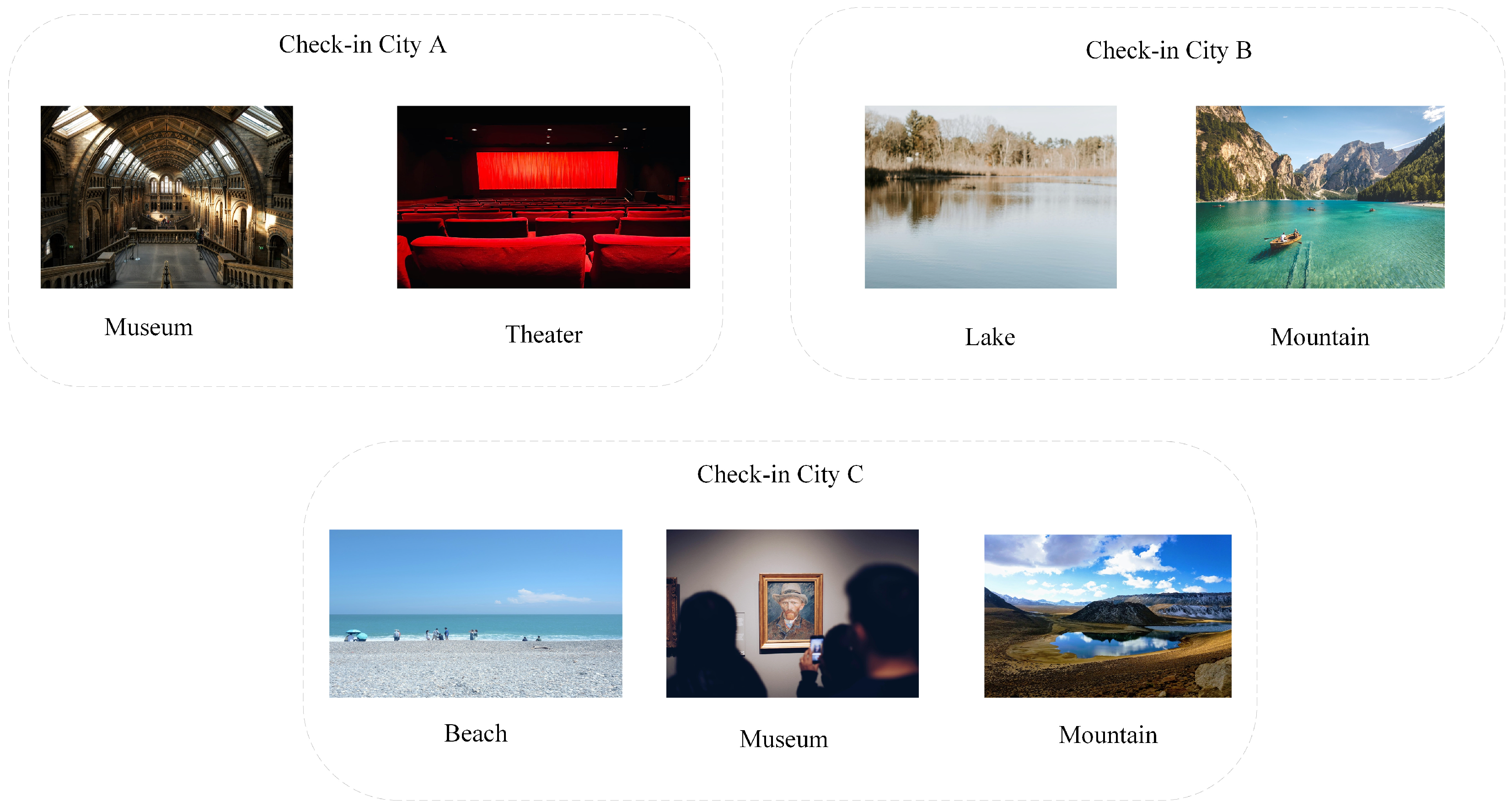
For a user, check-ins may occur in multiple cities. To better categorize a user’s multiple check-ins, it is essential to recognize that POI within the same city exhibit spatial similarity, adhering to the First Law of Geography. Similarly, POI in different cities may be interconnected due to their similar category information or because they have been checked into by the same user.

The check-in heterogeneous hypergraph comprises four distinct types of nodes $t{y}^4=\{u,v,g,c\}$. Each hyperedge includes four nodes, each belonging to a different type. This configuration distinguishes the POI checked into by the same user in different cities through city nodes. Additionally, POI from different cities are connected via user and category nodes.

The heterogeneous hyperedges in the check-in heterogeneous hypergraph are constructed based on users’ check-in records, reflecting the interactive relationships among different objects within the hyper-edges. Four distinct types of nodes are included in this heterogeneous hypergraph. Unlike homogeneous hypergraphs, there are two critical aspects of heterogeneous hypergraphs that must not be overlooked:

(1)

Indecomposability: In a heterogeneous hypergraph, hyperedges are typically indecomposable, meaning that the nodes within a hyperedge exhibit strong relationships, whereas the subset of nodes may not. For instance, in the “user, region, POI, category” cross-city POI recommendation model, the relationship between “user” and “category” is generally weak. Consequently, traditional hypergraph learning methods that decompose hyperedges cannot be employed;

(2)

Structural Preservation: Network embedding typically preserves local structures through observable relationships. However, due to network sparsity, many existing relationships are unobservable, and preserving the entire hypergraph structure solely through local structures is insufficient. Global structures, such as neighborhood structures, are also affected by data sparsity.

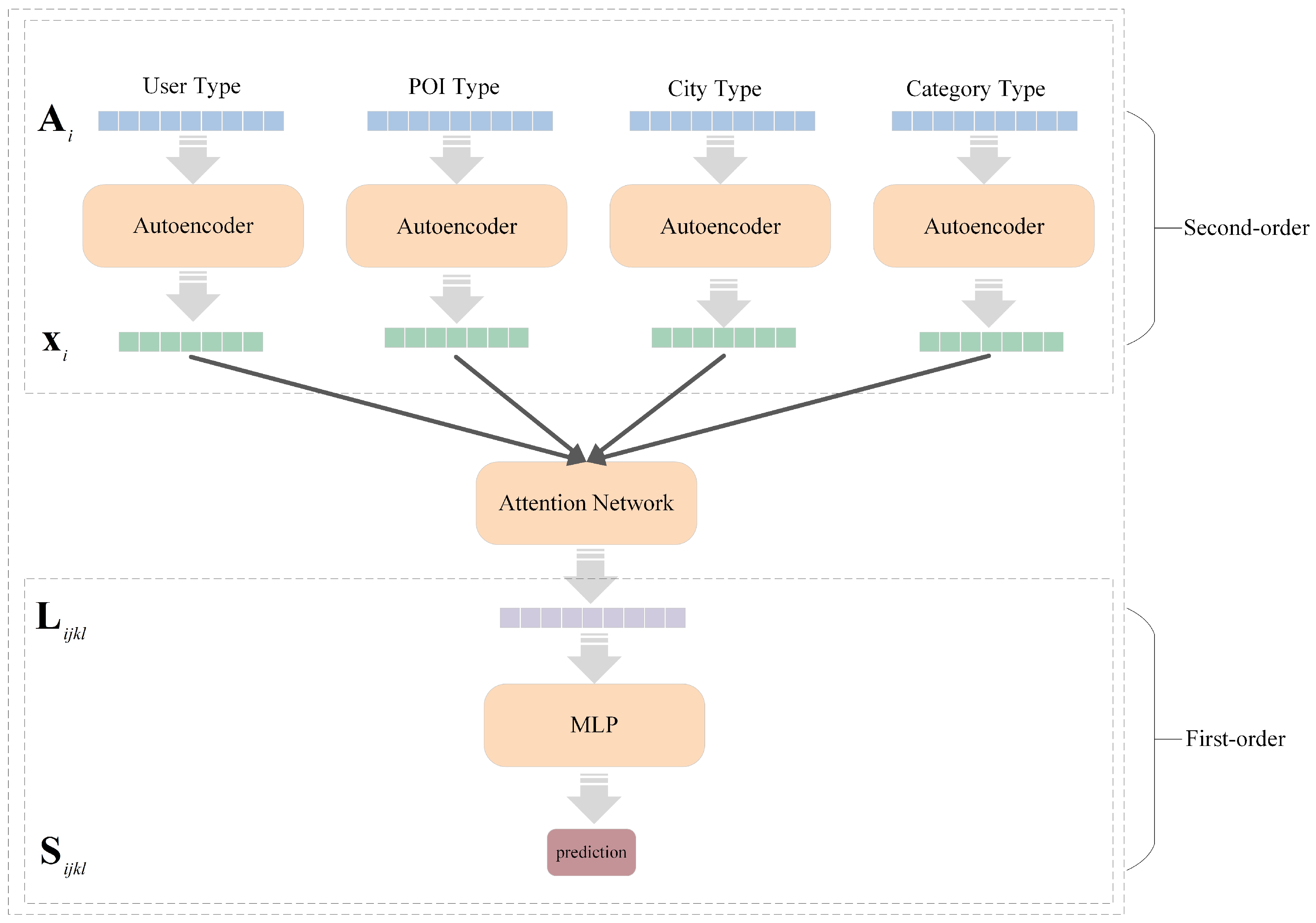
To address this, this paper proposes HHE, as shown in Figure 3.

For the check-in heterogeneous hypergraph, according to the theory presented in [22], it must satisfy both first-order and second-order similarities. Specifically, first-order similarity refers to the relationships between vertices within a hyperedge. 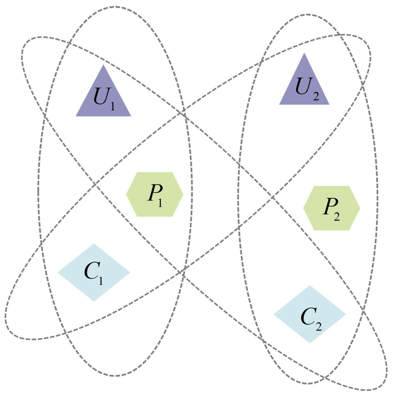For m nodes, if these m nodes $(n_1,n_2,\dots ,n_m)$ simultaneously exist within the same hyperedge and the subsets of these nodes do not form hyperedges, then these m nodes satisfy first-order similarity, which is defined as 1. Second-order similarity measures the similarity between the neighborhoods of nodes. To better illustrate second-order similarity, as shown in Figure 4, a dashed ellipse represents a heterogeneous hyperedge. In this example, the neighborhood nodes of $U_1$ include $\{(P_1,C_1),(P_1,C_2)\}$, and the neighborhood nodes of $U_2$ include $\{(P_1,C_1),(P_2,C_2)\}$. Since both $U_1$ and $U_2$ share the node $(P_1,C_1)$, both $U_1$ and $U_2$ satisfy second-order similarity.

Since, in cross-city POI recommendations, users may check in at the same point multiple times, a weight is assigned to each hyperedge $e_{hh}$ in the heterogeneous hypergraph ${\mathcal{G}}_{hh}$. A hyperedge weight matrix $\mathbf{W}$ of size $\left|{\mathcal{E}}_{hh}\right|\times \left|{\mathcal{E}}_{hh}\right|$ is defined, where ${\mathbf{W}}_{ii}$ represents the number of times that a user has checked in at a POI within the hyperedge $e_{hh}^i$, and ${\mathbf{W}}_{ij}=0$.

To obtain the adjacency matrix $\mathbf{A}$ of the heterogeneous hypergraph, it is necessary to define the incidence matrix $\mathbf{H}$ and the degree matrix ${\mathbf{D}}_v$ separately. The degree matrix ${\mathbf{D}}_v$ is derived from the hyperedge weight matrix $\mathbf{W}$ and the incidence matrix $\mathbf{H}$. The incidence matrix $\mathbf{H}$ has a size of $\left|Z\right|\times \left|{\mathcal{E}}_{hh}\right|$, where $\left|Z\right|=(\left|U\right|+\left|V\right|+\left|G\right|+\left|C\right|)$, and $h(z,e_{hh}^i)=1$ indicates $z\in e_{hh}^i$; otherwise, it equals 0. ${\mathbf{D}}_v$ is a diagonal matrix, with diagonal elements representing the degree of the corresponding vertices. The vertex degree is obtained by $d\left(z\right)=\sum _{e_{hh}\in {\mathcal{E}}_{hh}}w\left(e_{hh}\right)h(z,e_{hh})$, where $w\left(e_{hh}\right)$ represents the weight corresponding to hyperedge $e_{hh}$ in matrix $\mathbf{W}$.

The adjacency matrix $\mathbf{A}=\mathbf{H}{\mathbf{H}}^T-{\mathbf{D}}_v$, where the superscript T denotes the transpose of a matrix. The values in the adjacency matrix represent the co-occurrence frequency between two nodes. Each row of the adjacency matrix represents the neighborhood information of the current node. To better preserve the neighborhood information of the nodes, the nodes in the adjacency matrix are reencoded using an autoencoder [23], with the adjacency matrix as the input. The encoder and decoder are described by the following formulas:

$${\mathbf{x}}_i={\sigma }_e({\mathbf{W}}^{\left(1\right)}\ast {\mathbf{A}}_i+{\mathbf{b}}^{\left(1\right)})$$

(1)

$${\tilde{\mathbf{A}}}_i={\sigma }_d({\tilde{\mathbf{W}}}^{\left(1\right)}\ast {\mathbf{x}}_i+{\tilde{\mathbf{b}}}^{\left(1\right)})$$

(2)

Here, ${\mathbf{A}}_i\in R^{\left|Z\right|}$ is the i-th row of the adjacency matrix, ${\mathbf{W}}^{\left(1\right)}\in R^{d\times \left|Z\right|}$ and ${\tilde{\mathbf{W}}}^{\left(1\right)}\in R^{\left|Z\right|\times d}$ are weight matrices, ${\mathbf{b}}^{\left(1\right)}\in R^d$ and ${\tilde{\mathbf{b}}}^{\left(1\right)}\in R^{\left|Z\right|}$ are bias vectors, and $\sigma$ represents the Sigmoid function. ${\mathbf{x}}_i\in \mathbf{X}$; here, $\mathbf{X}$ is the embedding matrix of the nodes in the heterogeneous hypergraph.

The autoencoder has the capability to extract features and reconstruct encoding by minimizing the error between the input and output. This reconstruction process preserves the neighborhood information of nodes, thereby maintaining the second-order similarity between nodes. Since the adjacency matrix of the heterogeneous hypergraph is highly sparse, to accelerate the training speed of the model, only the non-zero elements of the adjacency matrix are reconstructed. The reconstruction error is shown as follows:

$$\mathcal{L}=\sum _{i\in \left|Z\right|}\left|\right|sign\left({\mathbf{A}}_i\right)\odot ({\mathbf{A}}_i-{\tilde{\mathbf{A}}}_i){\left|\right|}_F^2$$

(3)

Here, ⊙ represents element-wise multiplication, and $sign$ is the sign function.

Furthermore, the vertices in the heterogeneous hyperedges have different types. Considering that nodes of different types may have distinct embedding representations, each type of node has its own autoencoder. The reconstruction loss is shown as follows:

$${\mathcal{L}}_1=\sum _{t\in \{u,v,g,c\}}\sum _{i\in \{\left|U\right|,\left|V\right|,\left|G\right|,\left|C\right|\}}\left|\right|sign\left({\mathbf{A}}_i^t\right)\odot ({\mathbf{A}}_i^t-{\tilde{\mathbf{A}}}_i^t){\left|\right|}_F^2$$

(4)

Here, t is the number of node types.

By employing an attention network, the embeddings of four nodes $(v_i^u,v_j^v,v_k^g,v_l^c)$$({\mathbf{x}}_i^u,{\mathbf{x}}_j^v,{\mathbf{x}}_k^g,{\mathbf{x}}_l^c)\in R^d$ are used as inputs to obtain a joint embedding representation, as shown below:

$$\begin{array}{c}{\alpha }_j={\mathbf{q}}^{\mathrm{T}}\sigma \left({\mathbf{W}}^{\left(\mathbf{2}\right)}{\mathbf{h}}^t+{\mathbf{b}}^{\left(\mathbf{2}\right)}\right)\hfill \\ {\mathbf{L}}_{ijkl}={\displaystyle \sum _{t\in \{u,v,g,c\}}}{\alpha }_j{\mathbf{h}}^t\hfill \end{array}$$

(5)

Here, ${\mathbf{L}}_{ijkl}\in R^d$ represents the joint embedding, $\sigma$ is the Sigmoid function, and ${\mathbf{W}}^{\left(2\right)}\in R^{d\times d}$ and ${\mathbf{b}}^{\left(2\right)}\in R^d$ are the weight matrix and bias vector, respectively.

After obtaining $L_{ijkl}\in R^d$, it is mapped to a probability space through a non-linear layer to obtain the similarity:

$$S_{ijkl}=\sigma ({\mathbf{W}}^{\left(3\right)}\ast {\mathbf{L}}_{ijkl}+{\mathbf{b}}^{\left(3\right)})$$

(6)

Here $\sigma$ is the Sigmoid function, ${\mathbf{W}}^{\left(3\right)}\in R^{d\times d}$ and ${\mathbf{b}}^{\left(3\right)}\in R^d$ are the weight matrix and the bias vector, and the loss function is shown in the following equation:

$${\mathcal{L}}_2=-(R_{ijkl}log{S}_{ijkl}+(1-R_{ijkl})log(1-S_{ijkl}))$$

(7)

Define $R_{ijkl}$ to be 1 if there is a hyperedge between $(v_i^u,v_j^v,v_k^g,v_l^c)$; otherwise, it is 0. If $R_{ijkl}$ equals 1, the similarity $S_{ijkl}$ should be larger; otherwise, the similarity is smaller. In other words, first-order similarity is preserved.

Finally, to simultaneously preserve first-order and second-order proximities, Equations (4) and (7) are combined to derive the final loss function:

$${\mathcal{L}}_{{\mathcal{G}}_{hh}}=\beta {\mathcal{L}}_1+{\mathcal{L}}_2$$

(8)

Here, $\beta$ is a hyperparameter used to regulate the effect of ${\mathcal{L}}_1$ on total losses. The whole algorithm is shown in Algorithm 1.

Algorithm 1: Heterogeneous Hypergraph Embedding (HHE)

Input:  Check-in heterogeneous hypergraph ${\mathcal{G}}_{hh}$, Incidence matrix $\mathbf{H}$, Degree matrix ${\mathbf{D}}_v$, Adjacency matrix $\mathbf{A}$ Output:  Node embedding matrix $\mathbf{X}$ 1: Initialize the weight parameters ${\{{\mathbf{W}}^{\left(i\right)},{\mathbf{b}}^{\left(i\right)}\}}_{i=1}^3$ 2: while not converge do 3:    Encode the nodes of different types according to Equation (1) 4:    Decode according to Equation (2) 5:    Calculate the reconstruction loss according to Equation (4) 6:    Obtain the joint embedding of the four different types of nodes according to Equation (5) 7:    Calculate the similarity according to Equation (6) 8:    Compute the loss according to Equation (7) 9:    Calculate the joint loss function according to Equation (8) and update the parameters 10: end while 11: return the node embedding matrix $\mathbf{X}$

4.1.2. Source City Preference

To represent user preferences for the source city, a check-in aggregator network is utilized. After training, the heterogeneous hypergraph network for check-ins can be represented by the nodes within its heterogeneous hyperedges, as shown in the following equation:

$${\mathbf{e}}_{hh}=\mathrm{mean}\left({\mathbf{x}}_i^u+{\mathbf{x}}_j^v+{\mathbf{x}}_k^g+{\mathbf{x}}_l^c\right)$$

(9)

Here, ${\mathbf{e}}_{hh}$ is the embedding of the heterogeneous hyperedge. It is obtained by averaging the embedding representations of the contained nodes by bits.

User source city preferences can be derived by aggregating the hyperedges corresponding to all user check-in records. Utilizing attention mechanisms to achieve check-in aggregator network, the source city preference embedding is thus represented as follows:

$${\mathbf{u}}_i=\sum _{E_{h{h}_j}\in D_{u_i}}{\alpha }_j{\mathbf{e}}_{h{h}_j}$$

(10)

Here, ${\mathbf{u}}_i\in R^d$ denotes the source city preference of user i and ${\alpha }_j$ denotes the attention score of ${\mathbf{e}}_{h{h}_j}$. For the acquisition of the attention score, it is obtained by designing the attention network. This is expressed using the equation that follows:

$${\alpha }_j^{\prime }={\mathbf{q}}^{\mathrm{T}}\sigma \left(\mathbf{W}{\mathbf{e}}_{h{h}_j}+\mathbf{b}\right)$$

(11)

$${\alpha }_j={\displaystyle \frac{exp\left({\alpha }_j^{\prime }\right)}{{\sum }_{v_l\in D_{u_i}}exp\left({\alpha }_l^{\prime }\right)}}$$

(12)

Here, $\mathbf{q}\in R^d$ and $\mathbf{W}\in R^{d\times d}$ are the weight parameters of the attention network, $\mathbf{b}\in R^d$ is the bias vector, and $\sigma$ is the Sigmoid function.

4.2. Personalized Preference Transfer Module

In cross-city POI recommendations, users’ preferences in the target city may differ from those in their source city due to various local factors. For instance, in the context of dining, users may frequently check in at hotpot restaurants in their historical records when in their source city. However, upon arriving in the target city, their preferences might shift according to the city’s distinct characteristics. For example, in a city known for its seafood, users may be more inclined to check in at seafood restaurants. This shift in users’ preferences is referred to as preference transfer. Because different users check in at various locations in their source cities, their preferences also vary, resulting in diverse preferences once transferred to the target city. As a result, the process of preference transfer is inherently personalized. Additionally, since users may not have any historical check-in data in the target city, the cold-start problem becomes more pronounced in cross-city recommendation systems. However, personalized preference transfer can help mitigate this issue by learning users’ behavioral patterns in their source cities and inferring their potential preferences in the target city.

4.2.1. Users’ Transferable Features

Users’ transferable features are obtained by constructing a POI aggregator network. Each POI is associated with multiple textual descriptions, which facilitates the construction of a POI-category graph ${\mathcal{G}}_{vw}$ [10]. The POI embeddings are derived using the skip-gram.

Specifically, POI are treated as central words, and their corresponding descriptions are considered as context words, as illustrated in

Table 2. Correspondence between POI and words.

POI	Category	Skip-Grams
V1	Breakfast & Brunch, Restaurants	V1, Breakfast; V1, Brunch; V1, Restaurants
V2	Hotels & Travel, Car Rental	V2, Hotels; V2, Travel; V2, Car; V2, Rental
V3	Mexican, Restaurants	V3, Mexican; V3, Restaurants

. The initialization of POI embeddings is performed using Equation (13).

$$\begin{array}{cc}\hfill {\mathcal{L}}_{{\mathcal{G}}_{vw}}& =-\sum _{(v,w)\in {\mathcal{E}}_{vv}}logP\left(w\right|v)\hfill \\ \hfill & \approx -\sum _{(v,w)\in {\mathcal{E}}_{vw}}\left[log\sigma \left({\mathbf{y}}_w^T{\mathbf{y}}_v\right)+\sum _{w^{\prime }\notin W_v}log\sigma (-{\mathbf{y}}_{w^{\prime }}^T{\mathbf{y}}_v)\right]\hfill \end{array}$$

(13)

In this context, let v denote a POI, w represent the positive context associated with the POI, $w^{\prime }$ signify the negative context related to the POI, $W_v$ indicate the collection of all positive contexts for the POI v, ${\mathbf{y}}_w$ refer to the embedding for the word w, and ${\mathbf{y}}_v$ correspond to the embedding for POI.

Users’ transferable features are derived from the category information of POI where users have checked in, through the construction of a POI aggregator network. The importance of each POI in extracting transferable features is taken into account by employing an attention mechanism in the network. This mechanism compresses multiple POI into a single representation by assigning different weights to different parts based on their contributions. Consequently, each POI is weighted and summed using the attention mechanism:

$${\mathbf{p}}_{u_i}=\sum _{v_j\in D_{u_i}}{\beta }_j{\mathbf{y}}_j$$

(14)

Here, ${\mathbf{p}}_{u_i}\in R^d$ denotes the transferable features of user i, and ${\beta }_j$ represents the attention score of POI $v_j$, which can be interpreted as the importance of $v_j$ in the transferable features of the user. The attention scores are obtained by designing an attention network. The formulaic representation is as follows:

$${\beta }_j^{\prime }={\mathbf{q}}^{\mathrm{T}}\sigma \left({\mathbf{W}}^p{\mathbf{y}}_j+{\mathbf{b}}^p\right)$$

(15)

$${\beta }_j={\displaystyle \frac{exp\left({\beta }_j^{\prime }\right)}{{\sum }_{v_l\in D_{u_i}}exp\left({\beta }_l^{\prime }\right)}}$$

(16)

Here, $\mathbf{q}\in R^d$ and ${\mathbf{W}}^P\in R^{d\times d}$ are the weight parameters of the attention network, ${\mathbf{b}}^p\in R^d$ is the bias vector, and $\sigma$ is the Sigmoid function. The POI aggregator network obtains user transferable features as input to the meta-network, thereby generating weight parameters for the personalized transfer network.

4.2.2. Meta-Network

As previously discussed, user preferences in the target city vary. In other words, the preference transfer is personalized. There is a specific relationship between user preferences in the target city and a user’s transferable features. Inspired by the literature [24], a meta-network is designed through nonlinear mapping, which takes a user’s transferable features as input to obtain the weight parameters of the transition network. The meta-network is represented as follows:

$${\mathbf{W}}_{u_i}=\mathrm{Re}LU\left({\mathbf{W}}_2^m\sigma \left({\mathbf{W}}_1^m{\mathbf{p}}_{u_i}+{\mathbf{b}}_1^m\right)+{\mathbf{b}}_2^m\right)$$

(17)

Here, ${\mathbf{W}}_1^m\in R^{d\times d}$ and ${\mathbf{W}}_2^m\in R^{2d\times d}$ are the weight matrices of the parametric learning network, ${\mathbf{b}}_1^m\in R^d$ and ${\mathbf{b}}_2^m\in R^{2d}$ are the bias vectors, and $\sigma$ is the Sigmoid function.

4.2.3. Transfer Network

The input to the transfer network is the user’s source city preferences. Instead of being randomly initialized, the weight matrix of the transfer network is derived from the output of the meta-network. Since the meta-network provides an output for each user, each user in the transfer network possesses an independent weight matrix, thus enabling personalized preference transfer.

Based on the Embedding and Mapping Framework for Cross-Domain Recommendation (EMCDR) [24], an MLP is employed to complete the transfer network. The weight matrix ${\mathbf{W}}_{u_i}\in R^{2d}$ is reconstructed into ${\mathbf{W}}_{u_i}\in R^{d\times d}$. Thus, the transfer network is formulated as follows:

$${\mathbf{u}}_i^t=\mathrm{Re}LU\left({\mathbf{W}}_{u_i}{\mathbf{u}}_i+{\mathbf{b}}^t\right)$$

(18)

Here, ${\mathbf{W}}_{u_i}\in R^{d\times d}$ is the output of the parameter-learning network, ${\mathbf{b}}^t\in R^d$ is the bias vector of the transfer network, ${\mathbf{u}}_i\in R^d$ is the user preference obtained through Equation (10), and ${\mathbf{u}}_i^t\in R^d$ is the preference of user i after transfer, which corresponds to the user i preferences in the target city, i.e., the preferences for the target city.

4.3. Target City POI Recommendation Module

4.3.1. Target City POI Embedding

The geographical influence of POI in the target city aids in understanding users’ check-in behaviors at different locations [9]. Moreover, geographically proximate POI often share similar category attributes. Hence, each POI in the target city is initialized with a one-hot category vector, denoted as ${\mathbf{V}}^o={({\mathbf{v}}_1^o,{\mathbf{v}}_2^o,\dots ,{\mathbf{v}}_{D_2}^o)}^{\mathrm{T}}$. Subsequently, an undirected graph ${\mathcal{G}}_{geo}=({\mathcal{V}}^o,{\mathcal{E}}^o)$ is constructed based on the geographical relationships between POI, with edges $e_{i,j}^o\in {\mathcal{E}}^o$ defined as follows:

$$e_{i,j}^o=exp\left(-dist(v_i,v_j)\right)$$

(19)

$$dist(v_i,v_j)=2rarcsin\left(\sqrt{{sin}^2\left({\displaystyle \frac{la{t}_{v_2}-la{t}_{v_1}}{2}}\right)+cos\left(la{t}_{v_1}\right)cos\left(la{t}_{v_2}\right){sin}^2\left({\displaystyle \frac{lo{n}_{v_2}-lo{n}_{v1}}{2}}\right)}\right)$$

(20)

The $dist(·,·)$ represents the distance between POI $v_i$ and $v_j$. Here, r represents the radius of the Earth, $la{t}_{v_1}$ and $la{t}_{v_2}$ are the latitudes of the two points, and $lo{n}_{v_1}$ and $lo{n}_{v_2}$ are the longitudes of the two points. Using the distances between each pair of POI, an adjacency matrix ${\mathbf{A}}_{geo}$ can be constructed.

To capture the spatial relationships between POI, a GCN is used as follows:

$${\mathbf{V}}^{o^{\prime }}=\mathrm{ReLU}\left({\mathbf{A}}_{geo}{\mathbf{V}}^o\mathbf{W}+\mathbf{b}\right)$$

(21)

Here, $\mathbf{W}$ denotes the weight matrix and $\mathbf{b}$ is a bias term. ${\mathbf{V}}^o={\left({\mathbf{v}}_1^{o\prime },{\mathbf{v}}_2^{o\prime },\dots ,{\mathbf{v}}_{D_2}^{o\prime }\right)}^{\mathrm{T}}$ is the embedding matrix for the updated target city POI, which encodes the geographical and category information of the POI.

The representation of user preferences after transfer, denoted as ${\mathbf{u}}_i^t\in R^d$, is obtained according to Equation (18). Based on the concept of matrix factorization, the user’s rating of a POI can be viewed as the inner product of the transitioned user preference representation and the POI representation in the target city. Therefore, the score of user i for a POI in the target city is defined as follows:

$$s(i,j)={\left({\mathbf{u}}_i^t\right)}^{\mathrm{T}}{\mathbf{v}}_j^{o\prime }$$

(22)

According to the assumption of BPR [25], the probability of a previously visited POI being preferred is higher than that of an unvisited POI. By comparing two by two, the target city loss is

$${\mathcal{L}}_T=-\sum _{u\in \mathcal{U}}\sum _{j\in D_u^o}\sum _{k\notin D_u^o}log\sigma \left(s(i,j)-s(i,k)\right)$$

(23)

Here, $D_u^o$ are the check-in records of user u in the target city. $\sigma$ is the Sigmoid function.

4.3.2. Joint Training and Recommendation

By combining the heterogeneous hypergraph loss from Equation (8), the POI-Category graph loss from Equation (13), and the target city preference loss from Equation (23), the model is jointly trained in an end-to-end manner by minimizing the composite loss function:

$$\mathcal{L}={\lambda }_1{\mathcal{L}}_{{\mathcal{G}}_{hh}}+{\lambda }_2{\mathcal{L}}_{{\mathcal{G}}_{vw}}+{\lambda }_3{\mathcal{L}}_T$$

(24)

Here, ${\lambda }_1$, ${\lambda }_2$, and ${\lambda }_3$ are three hyperparameters that control the contribution of individual losses to the composite loss.

After optimizing the model parameters, the model can be used to recommend POI in the target city to users. Specifically, for a user $u^{\ast }\notin U$ and their historical check-in records, a preference representation ${\mathbf{u}}_{\ast }^t$ is generated following the transition of user interests. The rating of the target city POI for the user is then obtained by calculating the inner product of ${\mathbf{u}}_{\ast }^t$ and ${\mathbf{v}}_j^{o\prime }$.

$$s(\ast ,j)={\left({\mathbf{u}}_{\ast }^t\right)}^{\mathrm{T}}{\mathbf{v}}_j^{o\prime }$$

(25)

Finally, the top-k ranked target city POI can be selected as recommendations to user $u^{\ast }$ based on the estimated scores.

5. Experiments

5.1. Datasets and Evaluation Metrics

This study validates CHHPPT using real check-in datasets from Foursquare (https://sites.google.com/site/yangdingqi/home/foursquare-dataset) [15] and Yelp (https://www.yelp.com/dataset) [15]. The datasets are divided into 80% training set and 20% test set, and 50% training set and 50% test set. Detailed statistical information is shown in

Table 3. Statistics of datasets.

		Foursquare	Yelp
Total Data	Users	3305	81,403
	POI	45,382	96,995
	Check-ins	480,593	2,261,483
Cross-city	Users	1589	8362
Data	Check-ins	135,290	625,357

, which includes all the data required for inter-city analysis.

Foursquare. The Foursquare dataset is used, which is a check-in dataset where each check-in record is represented by user ID, check-in time, POI ID, POI name, latitude and longitude, city, state, country, and category. In the experiment, New York City (NY) was used as the target city, and California (CA) was considered as the user’s place of residence. The time span of the data ranges from January 2010 to December 2011.

Yelp. The Yelp dataset is derived from the Yelp Challenge dataset. Each check-in record is represented by user ID, business ID, city, state, latitude and longitude, category, and score. In the experiment, data from Las Vegas (LV) and Phoenix (PHX) were selected, with Las Vegas designated as the target city and Phoenix as the source city for users, and vice versa. The time span of the data ranges from 22 April 2005 to 13 December 2019.

In order to ensure data quality and enable the model to learn more useful information, the strategy in [14] is used to filter the dataset. POI with fewer than two check-ins are filtered out. Users who meet any of the following conditions will also be filtered out: (1) The user has fewer than five check-ins in their source city; (2) The user has fewer than two check-ins in their target city; (3) The pair ($\tilde{\mathrm{r}}$, $r_o$) appears fewer than ten times.

Evaluation Metrics. In this study, the model’s performance is evaluated using Mean Absolute Error (MAE) [26] and Root Mean Square Error (RMSE) [26]. MAE is suitable when the errors are relatively obvious, as larger errors carry higher weights. RMSE, on the other hand, is used when the errors are not as apparent, as shown in the following equations:

$$\mathrm{MAE}={\displaystyle \frac{{\displaystyle \sum _n^{i=1}}|y_i-{\widehat{y}}_i|}{n}}$$

(26)

$$RMSE=\sqrt{{\displaystyle \frac{{\displaystyle \sum _n^{i=1}}{(y_i-{\widehat{y}}_i)}^2}{n}}}$$

(27)

5.2. Baselines

We compare our proposed method with the other methods in

Table 4. Baselines.

Method Type	Method Name	Method Introduction
Traditional Recommendation Methods	TGT	TGT denotes the target MF model, which is trained only using target domain data.
Cross-city POI Recommendation Methods	TRAINOR [3]	TRAINOR employs a neural topic model to uncover users’ complex travel intentions for cross-city POI recommendations.
	CAPTOR [14]	CAPTOR utilizes spatial conditional random fields and collective behavior memory networks to recommend user pre-travel plans.
	CityTrans [4]	CityTrans framework leverages transfer learning to transfer travel knowledge from the home city to surrounding cities, balancing long-term preferences with short-term interest fluctuations.
Cross-Domain Recommendation Methods	CMF [27]	Collective Matrix Factorization (CMF) is an extension of MF. In CMF, user preference representations are shared between the source and target domains.
	EMCDR [24]	EMCDR is a cross-domain recommendation framework that addresses data sparsity by using a multi-layer perceptron to capture.
	DCDCSR [28]	Deep Framework for both Cross-Domain and Cross-System Recommendations (DCDCSR) is a neural network-based method for achieving user preference transfer. It accounts for the rating sparsity of individual users across different domains.
	SSCDR [29]	SSCDR is a Semi-Supervised Cross-Domain Recommendation method.

.

Furthermore, to evaluate the contribution of each module within the model, three variants of CHHPPT are presented as follows:

CHHPPT-MF: This variant removes the hypergraph module and derives user preferences based on matrix factorization, subsequently recommending POI to users.

CHHPPT-PA: This variant removes the POI aggregation network and replaces it with a multilayer perceptron.

CHHPPT-P: This variant eliminates the POI-category graph, representing POI through random initialization and disregarding POI category information.

CHHPPT-MP: This variant simultaneously removes both the hypergraph module and the POI-category graph.

5.3. Experimental Settings

The model framework was implemented using PyTorch (2.4.1 version), with baseline model parameters configured as per the original paper. For all embedding representations, the dimensionality d (i.e., embedding size) was fixed at 10. The parameters ${\lambda }_1$, ${\lambda }_2$, and ${\lambda }_3$ were set to 1. Learning was conducted using the Adam optimizer, with the learning rate tuned within the range 0.001, 0.003, 0.005, 0.01, 0.03, 0.05. For the three different recommendation tasks, batch sizes were set to 64 for CA-NY, and 128 for both LV-PHX and PHX-LV. Both the meta-network and the transfer network were designed as MLP. In Heterogeneous Hypergraph Embedding, $\beta$ is set to 1, using an autoencoder network structure with one hidden layer, with the size of the autoencoder’s hidden layer set to 32.

5.4. Empirical Analysis

Performance Comparison. This section presents a comprehensive analysis of the recommendation performance of the CHHPPT model across three tasks on two real-world datasets. The primary focus is on the recommendation accuracy of CHHPPT for these tasks. The percentages, 50% and 80%, represent the varying proportions of training and test datasets. The experimental results are presented in

Table 5. Recommended performance of CHHPPT on Yelp dataset.

	LV-PHX				PHX-LV
Ratio	50%		80%		50%		80%
Metric	MAE	RMSE	MAE	RMSE	MAE	RMSE	MAE	RMSE
TGT	4.5464	5.5077	4.3808	5.3322	4.5031	5.4538	4.4285	5.3513
CMF	3.8502	4.0594	3.1491	3.9531	4.3884	5.8191	3.7666	3.9829
DCDCSR	4.0321	4.5563	3.2586	3.9654	4.4454	5.1321	3.9542	4.1256
SSCDR	3.5987	3.6784	2.9951	3.8033	4.1311	4.5235	3.4101	3.9677
EMCDR	3.3153	3.5953	2.9638	3.7844	3.6395	3.9016	2.4771	3.2410
TRAINOR	3.0743	3.3340	2.7484	3.5120	3.4248	3.6328	2.3360	3.0054
CAPTOR	2.8512	3.0921	2.5489	3.2571	3.1762	3.3666	2.1665	2.7873
CityTrans	1.914	2.546	1.872	2.466	1.9826	2.7128	1.7741	2.0142
CHHPPT	1.5845	2.2462	1.3369	1.9433	1.6431	2.3597	1.3445	1.9127

and

Table 6. Recommended performance of CHHPPT on Foursquare dataset.

	CA-NY
Ratio	50%		80%
Metric	MAE	RMSE	MAE	RMSE
TGT	4.7901	5.8445	4.7686	5.7966
CMF	4.0240	4.9718	3.1491	3.9531
DCDCSR	3.9822	4.7895	3.2544	4.2355
SSCDR	3.5462	3.9512	2.9899	3.5621
EMCDR	3.3854	3.6655	2.6674	3.3201
TRAINOR	3.1393	3.3991	2.4735	3.0788
CAPTOR	2.9115	3.1680	2.3944	2.9803
CityTrans	2.7421	3.3211	2.3833	3.0124
CHHPPT	2.4760	3.1328	2.2538	2.8468

. Several observations can be drawn from the experimental results: (1) Overall, using 80% of the dataset as the training set yields better recommendation performance compared to using 50%. This improvement can be attributed to the larger training set enabling the model to learn more effectively; (2) Compared to cross-domain recommendation models, models focused on cross-city POI recommendation outperform cross-domain models in recommendation performance. This indicates that cross-domain models cannot be directly applied to cross-city POI recommendation without adjustments, as cross-city POI recommendation requires greater consideration of how geographical locations influence changes in user preferences; (3) TGT is a single-domain model that only uses data from the target region, and its recommendation performance is suboptimal. In comparison to TGT, all other recommendation methods can utilize data from the user’s source city, leading to better results. Therefore, leveraging data from the user’s source city is an effective method to mitigate data sparsity and improve performance in cross-city recommendations; (4) Compared to cross-city POI recommendation models, the overall recommendation performance of the CHHPPT model is superior. The reasons for this include, first, the effective construction of a personalized preference transfer module that better captures the varying preferences of different users in the target region and, second, the construction of a check-in heterogeneous hypergraph retains user check-in information from other cities, thereby addressing the impact of erroneous and missing information on user preferences in the source city. A better representation of source city preferences allows for the more accurate discovery of user preferences in the target city. At the same time, compared to the CityTrans model, it is shown that relying solely on the check-in sequence to uncover user preferences is insufficient. The category and location information of POI also play a crucial role in identifying user preferences.

The experimental results provide further insights into the model’s ability to handle data sparsity and the cold-start problem. The Heterogeneous Hypergraph Embedding technique plays a key role in capturing user preferences by constructing a check-in heterogeneous hypergraph network for the source city. This approach allows the hypergraph to simultaneously represent users, POI, and other types of relational nodes, which enhance the overall data representation by incorporating various relationships. Even in cases of data sparsity in the source city, the model mitigates the impact of missing information on preference mining by propagating information across multiple dimensions. In the user preference transfer module, the POI aggregation network extracts transferable user features from the historical records of multiple POI. This aggregation mechanism is crucial for alleviating the effects of data sparsity on personalized preference transfer, as it integrates information from the source city. As a result, it produces a more accurate mapping of user preferences, which can then be used for better recommendations in the target city. Additionally, by introducing a POI-geographical graph, the method combines geographical and categorical information of POI. This enables the model to not only address data sparsity but also to leverage spatial and categorical similarities, resulting in more reasonable recommendations for users.

The cold-start problem, which is often exacerbated by the lack of sufficient user–POI interaction data, is effectively mitigated through this approach. Through the heterogeneous hypergraph, CHHPPT integrates multiple types of information, such as relationships between users and POI, POI and categories, and geographical locations. This integration allows the model to make reliable inferences based on data from other dimensions, even when a user’s behavioral data in a new city are limited. For new users, CHHPPT can leverage historical data and user behavior from other cities to quickly establish an initial preference prediction. Thus, the personalized preference transfer mechanism successfully addresses the cold-start challenge for new users.

Ablation Analysis. As shown in

Table 7. Ablation on Yelp dataset.

	LV-PHX				PHX-LV
Ratio	50%		80%		50%		80%
Metric	MAE	RMSE	MAE	RMSE	MAE	RMSE	MAE	RMSE
CHHPPT-MP	2.2754	2.4565	2.1452	2.4321	2.3354	2.9611	2.0002	2.6159
CHHPPT-P	1.8433	2.3009	1.6433	2.0120	2.0988	2.4512	1.60734	2.1461
CHHPPT-PA	1.8532	2.4568	1.7455	2.1463	2.1011	2.5675	1.7211	2.2988
CHHPPT-MF	1.6236	2.2896	1.3205	1.9414	1.6307	2.3141	1.3847	1.9814
CHHPPT	1.5845	2.2462	1.3369	1.9433	1.6431	2.3597	1.3445	1.9127

and

Table 8. Ablation on Foursquare dataset.

	CA-NY
Ratio	50%		80%
Metric	MAE	RMSE	MAE	RMSE
CHHPPT-MP	3.1327	3.3875	2.5014	3.0633
CHHPPT-P	2.8433	3.3110	2.4433	2.9588
CHHPPT-PA	3.0121	3.3242	2.5123	3.1246
CHHPPT-MF	2.4915	3.1566	2.3454	2.9593
CHHPPT	2.4760	3.1328	2.2538	2.8468

, the ablation results for the four variant models on two datasets are presented. Overall, the performances of CHHPPT-MP, CHHPPT-P, and CHHPPT-PA are weaker than those of CHHPPT and CHHPPT-MF, with CHHPPT-MP exhibiting the lowest recommendation accuracy. This suggests that the transferable features of users are derived from the categories of the Points of Interest (POI), and the types of POI that users check into can significantly impact their preferences in the target city. Moreover, the check-in heterogeneous hypergraph preserves users’ check-in data from other cities, facilitating the identification of more complex, higher-order interactions between users and POI. This further underscores the influence of POI category information and check-in data on recommendation performance. The CHHPPT-P model highlights the benefit of learning from POI category data to better extract users’ transferable features. In addition, initializing POI embeddings based on category information can potentially improve the final recommendation performance. Finally, the CHHPPT-PA results demonstrate that employing an attention mechanism to construct a POI aggregation network helps identify which check-ins from users’ source cities are most valuable for extracting transferable features.

By comparing CHHPPT and CHHPPT-MF, it can be observed that CHHPPT outperforms CHHPPT-MF in recommendation performance. This suggests that constructing heterogeneous hyperedges helps to effectively mitigate the influence of erroneous and missing information in user preference mining. This also highlights the impact of check-ins outside the source city on user preferences. The heterogeneous hypergraph retains these additional check-ins, which allows for a more accurate extraction of user preferences from the source city. This, in turn, plays a positive role in mining user preferences for the target city. However, in certain cases, the recommendation performance declines. A possible explanation for this is the over-extraction of user preferences.

Embedding Size Analysis. The CHHPPT model was further investigated by varying the embedding sizes to 8, 10, 16, 32, 64, 128. The results for the Foursquare and Yelp datasets are summarized in Figure 5. For the embedding size comparison, the learning rates were set to 0.03 for the Yelp dataset and 0.01 for the Foursquare dataset, with a data split ratio of 8:2. It is evident that the optimal embedding size for both the Foursquare and Yelp datasets is 32. From the overall experimental results, it can be observed that, as the embedding size increases, the recommendation performance first improves and then declines. This occurs because, as the embedding dimension increases, more information can be incorporated. However, when the embedding size exceeds 32, the model’s recommendation performance starts to decline, indicating that the model is sensitive to the embedding dimension. When the embedding size reaches 128, the recommendation performance of the model decreases significantly. A higher embedding dimension not only includes more information but also introduces noisy data, which negatively affect recommendation performance. Therefore, for the UPPDOR model, the final selected embedding size is 32.

Learning Rate Analysis. The performance of the CHHPPT model was analyzed by varying the learning rates to 0.001, 0.003, 0.005, 0.01, 0.03, 0.05, as shown in Figure 6. In this section, the embedding size was fixed at 32, and the model’s performance was evaluated using MAE and RMSE metrics with a data split ratio of 8:2. Overall, the model’s performance in both MAE and RMSE metrics initially increased and then decreased with rising learning rates. In Figure 6a, the model exhibited optimal performance on the CA-NY task at a learning rate of 0.01, with a sharp decline at 0.05. For the LV-PHX and PHX-LV tasks, the best performance was observed at a learning rate of 0.03, with a decrease at 0.05. In Figure 6b, similar trends were observed across all three tasks, with a notable decline in performance at a learning rate of 0.05. Specifically, the CA-NY task showed optimal performance at a learning rate of 0.01, while the LV-PHX and PHX-LV tasks performed best at a learning rate of 0.03.

Hyperparametric Analysis. This section primarily examines the impact of hyperparameters ${\lambda }_1$, ${\lambda }_2$, and ${\lambda }_3$ on the model’s performance based on the MAE metric. During hyperparameter testing, the embedding size was fixed at 32. The learning rate was set to 0.01 for the Yelp dataset and 0.03 for the Foursquare dataset. Initially, ${\lambda }_1$ was varied while setting ${\lambda }_2={\lambda }_3={\displaystyle \frac{1-{\lambda }_1}{2}}$. The same strategy was applied to ${\lambda }_2$ and ${\lambda }_3$. As illustrated in Figure 7a–c, the MAE metric generally remained stable as ${\lambda }_1$, ${\lambda }_2$, and ${\lambda }_3$ increased from 0.1 to 0.9, with only slight variations observed for ${\lambda }_3$. Consequently, ${\lambda }_1$, ${\lambda }_2$, and ${\lambda }_3$ were ultimately set to 1.

6. Conclusions

This paper addresses the issues of erroneous information and incomplete data in user preference mining and the transfer of personalized user preferences. A novel framework, CHHPPT, for cross-city recommendation is proposed. Firstly, in the preference-mining module based on a heterogeneous hypergraph, user check-in records are utilized to construct a heterogeneous hypergraph with four types of nodes: users, POI, cities, and POI categories. User preferences for their source city are obtained through Heterogeneous Hypergraph Embedding. Secondly, in the personalized preference transfer module, a POI-category graph is constructed to obtain POI embeddings using the skip-gram method. Users’ transferable features are derived via a POI aggregator network. A meta-network is then built to learn the weight parameters of the transfer network, using the users’ transferable features as input. This network facilitates the user-personalized preference transfer from the source city to the target city. Lastly, in the target city POI recommendation module, a POI-geographical graph is constructed using the geographical information of the POI. This graph, combined with POI category information, is processed through a GCN to generate a joint embedding representation. The final recommendation is achieved by merging the personalized preference transfer embeddings with the target city’s POI embeddings. The efficacy of CHHPPT in enhancing recommendation accuracy was validated on two authentic LBSN datasets.

Although the current methods have addressed the issues of erroneous and missing information in user preference mining to some extent, and have also realized the personalized preference shift of users, several issues still remain:

(1)

Although this paper mainly focuses on medium-sized datasets, we acknowledge that, as the dataset size increases, the computational complexity and memory consumption of existing methods may rise significantly. Therefore, improving the scalability of algorithms to handle large-scale datasets, especially when the numbers of nodes and edges in hypergraphs increase substantially, is crucial. This could involve introducing more efficient graph processing algorithms or utilizing techniques such as graph sampling and hierarchical processing;

(2)

The potential sparsity of hypergraphs can indeed affect the performance of algorithms, particularly when edges and nodes are sparsely distributed. To address this issue, future research could consider adopting more flexible sparse matrix representation methods or exploring graph embedding techniques to mitigate the impact of sparsity;

(3)

User preferences for target cities are influenced by multiple factors, not merely by mining target city check-ins from users’ source city check-ins. In future research, we aim to explore additional auxiliary information to enrich both user and POI data. For example, factors such as the duration of users’ travel in different regions and the identification of regional characteristics could be utilized to provide more accurate and effective POI recommendations.